The subsurface-shear shaped solar $\alpha\Omega$ dynamo

Abstract

We propose a solar dynamo model distributed in the bulk of the convection zone with toroidal magnetic-field flux concentrated in a near-surface layer. We show that if the boundary conditions at the top of the dynamo region allow the large-scale toroidal magnetic fields to penetrate close to the surface, then the modeled butterfly diagram for the toroidal magnetic field in the upper convection zone is formed by the sub-surface rotational shear layer. The model is in agreement with observed properties of the magnetic solar cycle.

1 Introduction

It is widely believed that the 11-year sunspot activity is produced and organized by large-scale magnetic fields generated somewhere in the deep convection zone. Most of the solar dynamo models suggest that the toroidal magnetic field that emerges on the surface and forms sunspots is generated near the bottom of the convection zone, in the tachocline or just beneath it in a convection overshoot layer, (see, e.g., Choudhuri et al., 1995; Rüdiger & Brandenburg, 1995; Dikpati & Charbonneau, 1999; Bonanno et al., 2002; Tobias & Weiss, 2007). The belief in a deep-seated solar dynamo comes from the fact that this region is sufficiently stable, and can store magnetic flux despite the magnetic flux-tube buoyancy effect (Parker, 1975; Spiegel & Weiss, 1980; van Ballegooijen, 1982; Spruit & Roberts, 1983; van Ballegooijen & Choudhuri, 1988; Choudhuri, 1990). The tachocline represents a strong radial shear of the angular velocity. Yet, turbulent diamagnetism (see, e.g., Zeldovich, 1957 or Kitchatinov & Rüdiger, 1992) pumps the magnetic fields from the intensively mixed interior of convection zone to its boundaries. This effect can substantially amplify the toroidal magnetic fields near the convection zone boundaries, (see, e.g., Krivodubskij, 1987; Guerrero & de Gouveia Dal Pino, 2008).

However, an attention was drawn to a number of theoretical and observational problems concerning the deep-seated dynamo models (Brandenburg, 2005, 2006). A renewed discussion of the place of the solar dynamo can be found, e.g., in papers by Brandenburg (2005) and Tobias & Weiss (2007). In particular, there are some arguments that the sub-surface angular velocity shear could play an important role in the dynamo distributed in the convection zone. This shear layer becomes an important ingredient of the flux-transport dynamo models as well, (see, e.g., Guerrero & de Gouveia Dal Pino, 2008).

In this Letter we discuss the importance of the surface boundary conditions for the dynamo models, which include the subsurface shear layer. The boundary conditions commonly used in the dynamo models correspond to a perfect conductor at the bottom of the convection zone and vacuum boundary conditions at the top. Both the vacuum and perfect conductor boundary conditions can be regarded as a mathematically convenient idealization. The top boundary conditions play a particularly important role because they control the escape of the dynamo generated magnetic fields from the Sun.

The perfect conductor boundary condition is usually identified as “closed”, (e.g., Choudhuri, 1984), because in this case there is no penetration of the generated magnetic flux to the outside. For the axi-symmetric magnetic fields all magnetic field flux is closed inside the dynamo region. The vacuum boundary condition is identified as “open”. In this case the poloidal field lines are open to the outside, and the corresponding poloidal magnetic flux “freely” escapes. Also, the strength of the toroidal magnetic field goes smoothly to zero at the boundary. This means that the vacuum boundary condition does not allow to the toroidal field penetrate to the surface. With such boundary condition it is hardly possible to form sunspots from the near-surface large-scale toroidal magnetic fields.

Bearing in mind the dynamical nature of magnetic fields on the solar surface one can model the near-surface behaviour by using a combination of the “open” and “closed” types of the boundary conditions. Various consequences of this idea were explored, (see, e.g., Choudhuri, 1984; Tavakol et al., 1995; Covaset al., 1998; Kitchatinov & Mazur, 1999; Kitchatinov et al., 2000; Tavakol et al., 2002; Käpylä et al., 2010). Here, we apply this approach to a solar dynamo model that extends from the bottom of the convection zone to the top, including the region of the strong sub-surface rotational shear. We show that allowing the toroidal magnetic flux to penetrate to the surface brings the butterfly diagram of the toroidal large-scale magnetic field in the upper convection zone and also the phase relations between the different components of the dynamo-generated magnetic field in agreement with solar-cycle observations.

2 Dynamo equations

The evolution of the axi-symmetric magnetic field ($B$ being the azimuthal component of the magnetic field, $A$ is proportional to the azimuthal component of the vector potential) is governed by the following equations:

$$\frac{\partial A}{\partial t} = r\sin\theta\mathcal{E}_{\phi},$$ (1)

$$\frac{\partial B}{\partial t} = -\sin\theta\left(\frac{\partial\Omega}{\partial r}\frac{\partial A}{\partial\mu}-\frac{\partial\Omega}{\partial\mu}\frac{\partial A}{\partial r}\right)+\frac{1}{r}\frac{\partial r\mathcal{E}_{\theta}}{\partial r}+\frac{\sin\theta}{r}\frac{\partial\mathcal{E}_{r}}{\partial\mu},$$ (2)

where,

$$r\sin\theta\mathcal{E}_{\phi} = \psi_{\eta}\eta_{T}\left\{f_{2}^{(d)}+2f_{1}^{(a)}\right\}\frac{\partial^{2}A}{\partial r^{2}}+\psi_{\eta}\eta_{T}\left\{f_{2}^{(d)}+2f_{1}^{(a)}\right\}\frac{\left(1-\mu^{2}\right)}{r^{2}}\frac{\partial^{2}A}{\partial\mu^{2}}+$$

$$+ \psi_{\alpha}C_{\alpha}\eta_{T}Gf_{10}^{(a)}r\mu\sin\theta f\left(\theta\right)B$$

$$+ G\left(2f_{1}^{(a)}\mu\sin^{2}\theta\frac{\partial A}{\partial\mu}-\left(f_{3}^{(a)}-f_{1}^{(a)}\sin^{2}\theta\right)\frac{\partial A}{\partial r}\right)$$

$$\mathcal{E}_{r} = \frac{\eta_{T}\psi_{\eta}}{r}\left\{\left(f_{2}^{(d)}+2f_{1}^{(a)}\left(1-\mu^{2}\right)\right)\frac{\partial\sin\theta B}{\partial\mu}\right.$$

$$+ \left.2f_{1}^{(a)}\mu\sin\theta\frac{\partial}{\partial r}rB+2rGf_{1}^{(a)}\mu\sin\theta B\right\}$$

$$r\mathcal{E}_{\theta} = \eta_{T}\psi_{\eta}\left\{\left(f_{2}^{(d)}+2f_{1}^{(a)}\mu^{2}\right)\frac{\partial rB}{\partial r}\right.+$$

$$+ 2f_{1}^{(a)}\mu\sin\theta\frac{\partial}{\partial\mu}\left(\sin\theta B\right)$$

$$- \left.rG\left(f_{1}^{(a)}\cos 2\theta+f_{3}^{(a)}\right)B\right\}$$

These equations are similar to those used by Pipin & Seehafer (2009) and Seehafer & Pipin (2009). We use the same notations for the functions and parameters as in the paper of Pipin (2008) (hereafter, P08). Here, $G=\partial_{r}\log\rho$ is the density stratification scale. Functions $f_{1,2,3,10}^{(a,d)}$ depend on the Coriolis number $\Omega^{*}=2\tau_{c}\Omega_{0}$; functions $\psi_{\eta,\alpha}$ describe magnetic quenching and depend on $\beta=B/\sqrt{\mu_{0}\rho\bar{u^{2}}}$. For reference, these functions are given in Appendix. The parameter $C_{\alpha}$ controls the strength of the $\alpha$-effect. In the presented model the $\alpha$-effect is distributed in the bulk of the convection zone. For a more clear demonstration of the boundary condition impact, we confine the $\alpha$-affect in a low-latitude region where the radial gradient of the angular velocity is positive in the most part of the solar convection zone. Similarly to Dikpati et al. (2004) we specify the confinement function:

$$f(\theta)=\left(1+\mathrm{e}^{30\left(\left|\theta-\pi/2\right|-\pi/6\right)}\right)^{-1}.$$ (6)

In the radial direction the $\alpha$-effect depends on the density stratification, $G$, and function of the Coriolis number $f^{(a)}_{10}\left(\Omega^{*}\right)$. We introduce parameter $C_{\eta}$ to control the turbulent diffusion coefficient, $\eta_{T}=C_{\eta}\eta_{T}^{(0)}$, where $\eta_{T}^{(0)}=\tau_{c}\bar{u^{2}}/3$. The internal parameters of the solar convection zone are given by Stix (2002). At the top of the solar convection zone the stratification is strongly deviates from adiabatic, and also the turbulence parameters vary sharply. For this reason we confine the integration domain between 0.71$R_{\odot}$ and 0.972$R_{\odot}$ in radius, and it extends from the pole to pole in latitude. The differential rotation profile, $\Omega=\Omega_{0}f_{\Omega}\left(x,\mu\right)$ (shown in Fig.1a) is a slightly modified version of the analytical approximation proposed by Antia et al. (1998):

$$f_{\Omega}\left(x,\mu\right) = \frac{1}{\Omega_{0}}\left[\Omega_{0}+55\left(x-0.7\right)\phi\left(x,x_{0}\right)\phi\left(-x,-0.96\right)\right.$$

$$- \left.200\left(x-0.95\right)\phi\left(x,0.96\right)\right)$$

$$+ \left(21P_{3}\left(\mu\right)+3P_{5}\left(\mu\right)\right]\left(\frac{\mu^{2}}{j_{p}\left(x\right)}+\frac{1-\mu^{2}}{j_{e}\left(x\right)}\right)/\Omega_{0}$$

$$j_{p} = \frac{1}{1+\exp\left(\frac{0.709-x}{0.02}\right)},\,\,j_{e}=\frac{1}{1+\exp\left(\frac{0.692-x}{0.01}\right)}$$

where $\Omega_{0}=2.87\cdot 10^{-6}s^{-1}$ is the equatorial angular velocity of the Sun at the surface, $x=r/R_{\odot}$, $\phi\left(x,x_{0}\right)=0.5\left[1+\tanh\left[100(x-x_{0})\right]\right]$, $x_{0}=0.71$. The distribution of the Coriolis number, turbulent diffusivity and the RMS convection velocity are shown in Fig.1b. The radial profile of the $\alpha$-effect is shown in Fig.1c.

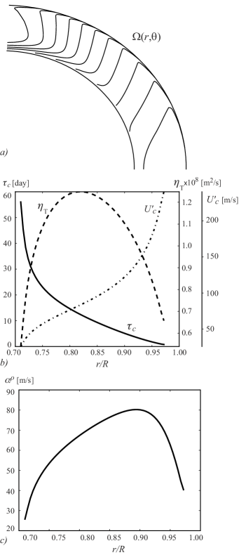
Figure 1: Internal parameters of the solar convection zone: a) the contours of the constant angular velocity are plotted for the levels $(0.75-1.05)\Omega_{0}$ with a step of $0.025\Omega_{0}$, see, Eq.(2); b) turnover convection time $\tau_{c}$, turbulent diffusivity $\eta_{T}$, RMS convective velocity $U^{\prime}_{c}$; c) the radial profile of the dynamo $\alpha$-effect, $\alpha^{\rho}=\eta_{T}Gf^{(a)}_{10}$, see Eq.(2). The distance is measured in units of the solar radius.

At the bottom of the integration domain we apply the perfect conductor ( “closed”) boundary conditions: $\mathcal{E}_{\theta}=0,\,A=0$. The boundary conditions at the top are defined as the following. Bearing in mind the idea of the partial escape of the toroidal flux from the Sun discussed in Introduction, we explore a combination of the “open” and “closed” boundary conditions at the top, controlled by a parameter $\delta$. For the toroidal field we use condition:

$$\delta\frac{\eta_{T}}{r_{e}}B+\left(1-\delta\right)\mathcal{E}_{\theta}=0.$$ (8)

This is similar to the boundary condition discussed by Kitchatinov et al. (2000). For the poloidal field we apply a combination of the local condition $A=0$ and condition of smooth transition from the internal poloidal field to the external potential (vacuum) field:

$$\delta\left(\left.\frac{\partial A}{\partial r}\right|_{r=r_{e}}-\left.\frac{\partial A^{(vac)}}{\partial r}\right|_{r=r_{e}}\right)+\left(1-\delta\right)A=0,$$ (9)

where the external potential field is :

$$A^{(vac)}\left(r,\mu\right)=\sum a_{n}\left(\frac{r_{e}}{r}\right)^{n}\sqrt{1-\mu^{2}}P_{n}^{1}\left(\mu\right),$$ (10)

$P_{n}^{1}\left(\mu\right)$ is the associated Legendre polynomial of degree $n$. For the numerical implementation of Eq.(9), we take a one-side finite difference approximation for the radial derivative at an angular mesh point $\mu_{j}$:

$$\left.\frac{\partial A_{j}}{\partial r}\right|_{r=r_{e}}=\frac{3A_{N\,j}-4A_{N-1\,j}+A_{N-2\,j}}{2h_{r}},$$

where $h_{r}$ is the radial discretization interval, and consider the expansion (10) at the top boundary $r=r_{e}$: $A_{N\,j}=\sum a_{n}\sqrt{1-\mu_{j}^{2}}P_{n}^{1}\left(\mu_{j}\right)$. Then, we define matrices $M_{nj}^{\left(a\right)}=\sqrt{1-\mu_{j}^{2}}P_{n}^{1}\left(\mu_{j}\right)$ and $\tilde{M}_{jn}=n\sqrt{1-\mu_{j}^{2}}P_{n}^{1}\left(\mu_{j}\right)$, with $\mu_{j}$ being collocation points of $P_{n}^{1}$ (see, Boyd, 2001). This procedure allows us to express coefficients $a_{n}$ in (10) via the values of potential $A$ at the grid-points: $a_{n}=M_{nj}^{\left(a\right)-1}A_{N\,j}$. Substituting this in Eq.(9) and solving it we get :

$$A_{N\,j}=\delta\left(3E_{jk}+2h_{r}\tilde{M}_{jk}M_{nk}^{\left(a\right)-1}\right)^{-1}\left(4A_{N-1\,jk}-A_{N-2\,k}\right),$$

where $E$ is a unit diagonal matrix.

3 Results and discussion

Parameter $\delta$ in the boundary conditions describes a transition between the “closed” ($\delta=0$) to “open” ($\delta=1$) boundaries. Physically, it controls penetration of the dynamo-generated fields into the outer atmosphere.

Decreasing $\delta$ in Eqs.(8,9) results in stronger tangential and weaker radial large-scale magnetic fields at the surface. While the strong toroidal magnetic field is a desired feature of the model, the weak radial magnetic field decreases the efficiency of the radial subsurface shear to produce large-scale toroidal magnetic fields. In fact, the simulations reveal that the critical dynamo number, $C_{\alpha}$, is greater when the penetration parameter $\delta$ is smaller. For this reason we consider the case of a small deviation from the vacuum ( “open”) boundary conditions. Moreover, in order to match the dynamo period to the solar cycle we choose the magnetic diffusivity parameter $C_{\eta}=0.05$, which is significantly lower then the value predicted by the mixing length theory. To demonstrate the effect of the new boundary conditions with the field penetration we show for comparison in Figure 2 and 3 the results of two runs for $\delta=0.95$ (corresponding to a partial penetration of toroidal field) and $\delta=1$ (the vacuum boundary conditions).

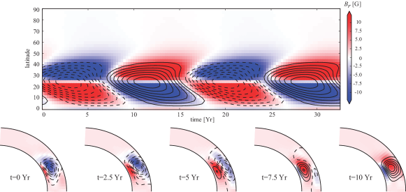
Figure 2: The case of $\delta=0.95$ (the top boundary conditions with a partial penetration of toroidal magnetic fields into the outer layers of the Sun). The top panel shows the near-surface toroidal component of large-scale magnetic fields (contour lines) and the surface radial component of the field (color background). The bottom panel shows snapshots of the poloidal (contour lines) and toroidal magnetic field components for a half of the magnetic cycle. The maximum strength of the toroidal field is about 1KG. Time is in years.

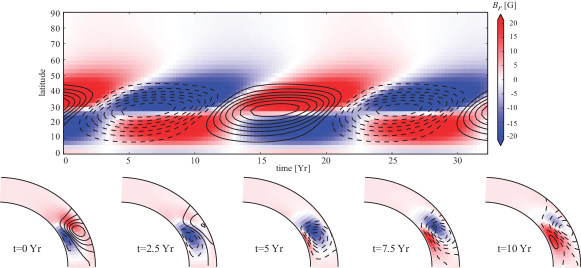
Figure 3: The same as in on the Fig.2 for the vacuum boundary conditions, $\delta=1$.

These results show that allowing the large-scale toroidal magnetic field to penetrate in to the surface layers of the Sun changes the direction of the latitudinal migration of the toroidal field activity and produces the magnetic butterfly diagram in a good qualitative agreement with solar-cycle observations. The dynamo-wave penetrates to the surface and propagates along the iso-surface of angular velocity in the subsurface shear layer. This is in agreement with the Yoshimura rule (Yoshimura, 1975).

Dikpati et al. (2002) explored generation of toroidal magnetic fields by the $\Omega$-effect in the sub-surface shearlayer in the Babcok-Leighton-type dynamo models. They found that the phase relation between the sub-surface toroidal magnetic field and the surface radial magnetic field is inconsistent with observations. We believe that this inconsistency was because in their model the source of the surface poloidal magnetic fields was related with the bottom of convection zone. Therefore, the sub-surface toroidal field that is generated in the sub-surface shear layer does not contribute directly to the generation of the poloidal magnetic field.

Both of our simulation runs were started with the initial magnetic fields with of the equally mixed symmetrical and antisymmetrical realtive to the equator components. The evolution retains only the dipole-like parity configurations in both cases though the relaxation time in the penetration case of $\delta=0.95$ is much longer than in the case of the pure vacuum boundary conditions. If we relax the confinement of the alpha-effect in latitude, i.e., $f(\theta)=1$ instead of Eq.(6), the general patterns of Fig.2 are hold except that the maximum of the toroidal magnetic field is shifted to higher latitude $\approx 40^{\circ}$. Therefore we can conclude that the $\alpha\Omega$- dynamo model with the boundary conditions that allow a small partial penetration of the toroidal field into the outer layers of the Sun, can robustly reproduce the solar-cycle butterfly diagram for the near-surface large-scale magnetic field evolution. These results demonstrate the importance of the subsurface rotational shear layer in the solar dynamo mechanism.

4 Acknowledgements

This work was supported by the NASA LWS NNX09AJ85G grant and partially by the RFBR grant 10-02-00148-a.

4.1 Appendix

Here, we give the definitions of the functions which were used in the model. The given functions describe the efficiency of the Coriolis force and the mean magnetic field to act on the stratified turbulence and to produce the dynamo $\alpha$-effect, anisotropy of magnetic diffusion, turbulent magnetic pumping, magnetic quenching of the turbulent effects, etc. These effects are discussed in (Pipin, 2008). Functions $f_{1,2,3,10}^{(a,d)}$ depend on the Coriolis number $\Omega^{*}=2\tau_{c}\Omega_{0}$; functions $\psi_{\eta,\alpha}$ describe magnetic quenching and depend on $\beta=B/\sqrt{\mu_{0}\rho\bar{u^{2}}}$:

$$f_{1}^{(a)} = \frac{3}{4\Omega^{*\,2}}\left(\left(\Omega^{*\,2}+3\right)\frac{\arctan\Omega^{*}}{\Omega^{*}}-3\right),$$

$$f_{2}^{(d)} = \frac{3}{4\Omega^{*\,2}}\left(\left(\left(\varepsilon-1\right)\Omega^{*\,2}+3\varepsilon+1\right)\frac{\arctan\left(\Omega^{*}\right)}{\Omega^{*}}-\left(3\varepsilon+1\right)\right),$$

$$f_{3}^{(a)} = \frac{3}{4\Omega^{*\,2}}\left(\left(\left(\varepsilon-1\right)\Omega^{*\,2}+\varepsilon-3\right)\frac{\arctan\Omega^{*}}{\Omega^{*}}+3-\varepsilon\right),$$

$$f_{10}^{(a)} = -\frac{1}{3\Omega^{*\,3}}\left(3\left(\Omega^{*2}+1\right)\left(\Omega^{*2}+\varepsilon-1\right)\frac{\arctan\Omega^{*}}{\Omega^{*}}-\left(\left(2\varepsilon+1\right)\Omega^{*2}+3\varepsilon-3\right)\right),$$

$$\psi_{\eta} = \frac{3}{16\beta^{2}}\left(\left(\left(4\beta^{2}+3\right)\varepsilon+4\beta^{2}-1\right)\frac{\arctan\left(2\beta\right)}{2\beta}+1-3\varepsilon\right)$$

$$\psi_{\alpha} = \frac{5}{128\beta^{4}}\left(16\beta^{2}-3-3\left(4\beta^{2}-1\right)\frac{\arctan\left(2\beta\right)}{2\beta}\right).$$

The parameter $\varepsilon$ measures the ratio between the turbulent energies of the kinetic and magnetic fluctuations $\varepsilon=\bar{b^{2}}/\mu_{0}\rho\bar{u^{2}}$, in the background turbulence (in the absence of the mean-fields). Note, in notation of Pipin(2008), the turbulent diffusivity and $\alpha$-effect quenchning functions are defined as follows, $\psi_{\eta}=\phi_{3}+\phi_{2}-2\phi_{1}$, and $\psi_{\alpha}=-3/4\phi^{(a)}_{6}$, respectively. Expressions for $\phi_{1,2,3}$ and $\phi^{(a)}_{6}$ are given in (Pipin, 2008).

References

- Antia et al. (1998) Antia, H. M. , Basu, Sarbani, Chitre, S. M. 1998, MNRAS, 298,543
- Boyd (2001) Boyd, J.P., 2001, Chebyshev and Fourie Spectral Methods, 2nd ed.(Mineola, N.Y.: Dover Publications)
- Brandenburg (2006) Brandenburg, A. 2006, ASP Conference Series, 354,Solar MHD Theory and Observations: A High Spatial Resolution Perspective, 121
- Brandenburg (2005) Brandenburg, A.,2005, ApJ, 625, 539
- Brandenburg & Subramanian (2005) Brandenburg, A., Subramanian, K..2005, Phys. Rep. 417, 1
- Bonanno et al. (2002) Bonanno, A., Elstner, D., Rüdiger, G., 2002, A&A, 390, 673
- Choudhuri et al. (1995) Choudhuri, A. R., Schüssler, M., & Dikpati, M. 1995, A&A, 303, L29
- Choudhuri (1984) Choudhuri, A. R. 1984, ApJ, 281, 846
- Choudhuri (1990) Choudhuri, A. R. 1990, ApJ, 355, 733
- Covaset al. (1998) Covas, E., Tavakol, R., Tworkowski, A., Brandenburg, A. 1998, A&A, 329, 350
- Dikpati & Charbonneau (1999) Dikpati, M., & Charbonneau, P. 1999, ApJ, 518, 508
- Dikpati et al. (2002) Dikpati, M., Corbard, T., Thompson, M.J., Gilman, P. 2002, ApJ,575,L41
- Dikpati et al. (2004) Dikpati, M., de Toma, G., Gilman, P.A., Arge, C.N., White, O.R. 2004, ApJ,601,1136
- Guerrero & de Gouveia Dal Pino (2008) Guerrero, G., de Gouveia Dal Pino, E. M. 2008, A&A, 485, 267
- Käpylä et al. (2010) Käpylä, P.J., Korpi, M.J. & Brandenburg, A. 2010, A&A, 518, 22
- Kitchatinov & Rüdiger (1992) Kitchatinov, L.L., Rüdiger, G. 1992, A&A,260, 494
- Kitchatinov & Mazur (1999) Kitchatinov, L.L., Mazur, M.V. 1999, AstL,25, 471
- Kitchatinov et al. (2000) Kitchatinov, L. L., Mazur, M. V., Jardine, M., 2000, A&A, 359, 531
- Krivodubskij (1987) Krivodubskij, V. N., 1987, SvAL,13, 338
- Parker (1975) Parker, E.N., 1975, ApJ, 198, 205
- Pipin & Seehafer (2009) Pipin, V.V. & Seehafer, N. 2009, A&A, 493,819
- Pipin (2008) Pipin, V. V. 2008, Geophys. Astrophys. Fluid Dynam., 102, 21
- Rüdiger & Brandenburg (1995) Rüdiger, G., Brandenburg, A., 1995, A&A, 296, 557
- Seehafer & Pipin (2009) Seehafer, N. & Pipin, V.V. 2009, A&A, 508,9
- Spiegel & Weiss (1980) Spiegel, E.A., & Weiss, N.O., 1980, Nature, 287, 616
- Spruit & Roberts (1983) Spruit, H.C., & Roberts, B., 1983, Nature, 304, 401
- Stix (2002) Stix, M. 2002, The Sun. An Introduction, 2nd Ed. (Berlin: Springer)
- Tavakol et al. (1995) Tavakol, R.K., Tworkowski, A. S., Brandenburg, A., Moss, D., Tuominen, I., 1995, A&A, 296, 269
- Tavakol et al. (2002) Tavakol, R.; Covas, E.; Moss, D.; Tworkowski, A. 2002 A&A, 387, 1100
- Tobias & Weiss (2007) Tobias, S. & Weiss, N. 2007, in “The Solar Tachocline”, eds by Hughes,D.W., Rosner, R. and Weiss N.O., CUP, Cambridge, UK, p.319
- van Ballegooijen (1982) van Ballegooijen, A. A. 1982, A & A, 113, 99
- van Ballegooijen & Choudhuri (1988) van Ballegooijen, A.A., Choudhuri, A.R. 1988, ApJ, 333, 965
- Zeldovich (1957) Zeldovich, Ya.B. 1957, Sov.Phys. JETP, 4, 460
- Yoshimura (1975) Yoshimura, H. 1975 ApJ, 201, 740