Nuclear size correction to the Lamb shift of one-electron atoms

Vladimir A. Yerokhin Center for Advanced Studies, St. Petersburg State Polytechnical University, Polytekhnicheskaya 29, St. Petersburg 195251, Russia
Abstract

The nuclear size effect on the one-loop self energy and vacuum polarization is evaluated for the $1s$, $2s$, $3s$, $2p_{1/2}$, and $2p_{3/2}$ states of hydrogen-like ions. The calculation is performed to all orders in the binding nuclear strength parameter ${Z\alpha}$. Detailed comparison is made with previous all-order calculations and calculations based on the expansion in the parameter ${Z\alpha}$. Extrapolation of the all-order numerical results obtained towards $Z=1$ provides results for the radiative nuclear size effect on the hydrogen Lamb shift.

pacs:
31.30.jf, 12.20.Ds, 31.15.A-

Introduction

The distribution of charge of the nucleus influences the Dirac energies of atomic systems as well as the quantum electrodynamical corrections to the energy levels. This effect, termed as the nuclear size (NS) correction, is important for comparison of theoretical predictions with experimental data for the whole range of the nuclear charges $Z$, from hydrogen ($Z=1$) up to uranium ($Z=92$). The NS corrections to the one-loop self energy and vacuum polarization have been previously investigated both within the approach based on the expansion in the nuclear binding strength parameter ${Z\alpha}$ friar:79 ; hylton:85 ; pachucki:93:density ; milstein:03:fns ; jentschura:03:jpa ; milstein:04 (where $\alpha$ is the fine structure constant) and within the numerical approach that accounts the parameter ${Z\alpha}$ to all orders soff:88:vp ; mohr:93:prl . In the high-$Z$ region, the numerical all-order approach provides accurate predictions for the NS effect on the radiative corrections. For lower $Z$, however, the NS effect diminishes and becomes increasingly more difficult to identify in a numerical calculation. On the contrary, the ${Z\alpha}$-expansion approach provides accurate predictions for the low-$Z$ ions and only the qualitative estimates in the high-$Z$ region. A quantitative cross-check of the two complementary approaches is not simple and has not been accomplished up to now.

The NS corrections became of particular interest recently, after the results of the muonic hydrogen Lamb-shift experiment were announced pohl:10 . It turned out that the value for the proton charge radius $r_{p}$ deduced from the muonic hydrogen differs by five standard deviations from the spectroscopic value of $r_{p}$ derived from the hydrogen atom. This unexplained disagreement stimulates the scientific community to double-check all contributions originating from the nuclear charge distribution, both for the muonic and normal atoms.

The aim of the present investigation is to perform an accurate numerical all-order calculation of the NS correction to the one-loop self energy and vacuum polarization and to make a detailed comparison with the ${Z\alpha}$-expansion results available.

The relativistic units ($m$ = $\hbar=c=1$) and the charge units $\alpha=e^{2}/(4\pi)$ are used in this paper.

I NS correction to Dirac energy

The leading-order NS correction to the energy levels of a hydrogen-like atom is defined as the difference of the corresponding eigenvalues of the Dirac equation with the point-Coulomb and the extended-nucleus potentials. The two most commonly used models of the nuclear charge distribution are the uniformly charged sphere (“sph”) and the two-parameter Fermi (“Fer”) model,

$\displaystyle\rho_{\rm sph}(r)=\rho_{0}\,\theta(R_{\rm sph}-r)\,,$ (1)
$\displaystyle\rho_{\rm Fer}(r)=\frac{\rho_{0}}{1+\exp[(r-c)/a]}\,,$ (2)

where $R_{\rm sph}=\sqrt{5/3}\,R$ is the radius of the sphere with the root-mean-square (rms) radius $R$, $c$ and $a$ are the parameters of the Fermi distribution, and $\rho_{0}$ are the normalization factors. The parameter $a$ of the Fermi distribution is standardly fixed by $a=2.3/(4\ln 3)$ fm. For a given value of the rms radius, the parameter $c$ can be determined by the simple approximate formula

$\displaystyle c^{2}\approx\frac{5}{3}R^{2}-\frac{7}{3}a^{2}\pi^{2}\,.$ (3)

In the calculations performed in this work, we will assume that the parameter $c$ of the Fermi distribution is fixed exactly by the above formula.

For the uniformly charged sphere model, the Dirac equation can be solved analytically shabaev:93:fns . In this case, the NS correction to the Dirac energy is represented in terms of the hypergeometric function. While the exact expression is rather cumbersome, simple approximate expressions for the NS correction obtained in Ref. shabaev:93:fns are highly useful. For the general model of the nuclear charge distribution, the NS correction can be easily obtained by numerical solution of the Dirac equation. Numerical results are conveniently parameterized in terms of the function ${G}_{\rm N}({Z\alpha},R)$, whose definition is inspired by the analytic relativistic results shabaev:93:fns ,

$\displaystyle\Delta E_{\rm N}(ns)$ $\displaystyle\ =\frac{({Z\alpha})^{2}}{n}\,\left(\frac{2{Z\alpha}R_{\rm sph}}{n}\right)^{2\gamma}\,\frac{1}{10}\,{G}_{N}({Z\alpha},R)\,,$ (4)
$\displaystyle\Delta E_{\rm N}(np_{1/2})$ $\displaystyle\ =\frac{({Z\alpha})^{4}}{n}\,\left(\frac{2{Z\alpha}R_{\rm sph}}{n}\right)^{2\gamma}\,\frac{n^{2}-1}{40n^{2}}\,{G}_{N}({Z\alpha},R)\,,$ (5)

where $\gamma=\sqrt{1-({Z\alpha})^{2}}$ and $R_{\rm sph}$ is the radius of the sphere with the rms radius $R$. The function ${G}_{N}({Z\alpha},R)$ is a slowly varying function of ${Z\alpha}$ and $R$ and its numerical values are of order of unity.

The numerical results obtained for the NS correction with the Fermi model of the nuclear charge distribution are listed in Table Acknowledgments. The numerical evaluation was performed by solving the Dirac equation with help of the RADIAL package salvat:95:cpc and, independently, by using the B-spline finite basis set method shabaev:04:DKB . For calculations in the low-$Z$ region, the RADIAL package was upgraded into the quadruple arithmetics (about 32 digits). The values of the rms charge radii used were taken from the compilation angeli:04 for all ions except for uranium; the uranium rms radius was taken from Ref. kozhedub:08 .

II NS correction to self energy

The one-loop self-energy contribution to the Lamb shift is given by a matrix element of the self-energy operator with the mass renormalization part subtracted,

$\displaystyle\Delta E_{\rm SE}=\bigl{<}a\bigl{|}\gamma^{0}\widetilde{\Sigma}(\varepsilon_{a})\bigr{|}a\bigr{>}\,,$ (6)

where $\widetilde{\Sigma}(\varepsilon)=\Sigma(\varepsilon)-\delta m$ and $\delta m$ is the mass counterterm. The self-energy operator is mohr:98

$\displaystyle\Sigma(\varepsilon,\bm{x}_{1},\bm{x}_{2})=2i\alpha\gamma^{0}\int^{\infty}_{-\infty}d\omega\,$ $\displaystyle\,D^{\mu\nu}(\omega,x_{12})\,$
$\displaystyle\times\alpha_{\mu}G(\varepsilon-\omega,\bm{x}_{1},\bm{x}_{2})\alpha^{\nu}\,,$ (7)

where $D^{\mu\nu}$ is the photon propagator, $G$ is the Dirac-Coulomb Green function, $G(\varepsilon)=(\varepsilon-H)^{-1}$, $H$ is the Dirac-Coulomb Hamiltonian, and $\alpha^{\mu}=\gamma^{0}\gamma^{\mu}$ are the Dirac matrices. The nuclear-size self-energy (NSE) correction is defined as the difference between the matrix elements (6) evaluated with the point-Coulomb potential and the potential of the extended-charge nucleus.

Numerical, all-order (in ${Z\alpha}$) evaluation of the one-loop self-energy correction have been extensively discussed in the literature over past decades mohr:74:a ; blundell:91:se ; mohr:93:prl ; jentschura:99:prl ; cheng:93 ; yerokhin:99:pra , both for the case of the point-Coulomb and extended-nucleus potentials. In the present investigation, we employ the method developed in our previous work yerokhin:05:se for the case of the point nucleus. This method can be immediately extended to a general (local and spherically-symmetrical) potential, provided that one can calculate the Green function of the Dirac equation with this potential. (Beside the full Green function, the one-potential Green function is also needed in actual calculations.) In the present work, we develop an efficient scheme of computation of the Dirac Green function for a general potential, which is described in Appendix A for the full Green function and Appendix B for the one-potential Green function.

The main advantage of the method reported in Ref. yerokhin:05:se is a fast convergence of the partial-wave expansion of the matrix element (6). In the present work, we calculate the difference between the point-nucleus and extended-nucleus matrix elements. For this difference, the partial-wave expansion converges even faster (especially, in the low-$Z$ region) than for the self-energy correction. Because of this, we were able to significantly improve numerical accuracy as compared to results previously reported in the literature.

Numerical results for the NSE correction to the energy shift are usually parameterized in the same way as the one-loop self-energy itself,

$\displaystyle\Delta E_{\rm NSE}=\frac{\alpha}{\pi}\,\frac{({Z\alpha})^{4}}{n^{3}}\,F_{\rm NSE}({Z\alpha},R)\,.$ (8)

Comparison of the present results with those by Mohr and Soff mohr:93:prl for the homogeneously charged sphere model is given in Table Acknowledgments. Numerical results obtained in the present work with the Fermi model of the nuclear charge distribution are summarized in Table Acknowledgments.

The leading dependence of the NSE correction on $R$ and ${Z\alpha}$ can be conveniently factorized out in terms of the first-order NS contribution $\Delta E_{\rm N}$,

$\displaystyle\Delta E_{\rm NSE}(njl)=\Delta E_{\rm N}(n\nicefrac{{1}}{{2}}l)\,\frac{\alpha}{\pi}\,{G}_{\rm NSE}(njl)\,,$ (9)

where $\Delta E_{\rm N}$ is given by Eqs. (4) and (5). An important feature of this parametrization milstein:02:prl ; milstein:04 is that it involves the full NS correction, rather than only the leading term of its ${Z\alpha}$ expansion. With such choice of normalization, ${G}_{\rm NSE}$ is a slowly-varying function of $Z$ and its dependence on $R$ is more tractable. Note that for the $np_{3/2}$ reference state, Eq. (9) has $\Delta E_{\rm N}(np_{1/2})$ as a prefactor, which was suggested in Ref. milstein:04 . The ${Z\alpha}$ expansion of the function ${G}_{\rm NSE}$ has the form

$\displaystyle{G}_{\rm NSE}(ns)=$ $\displaystyle\,({Z\alpha})\,a_{10}+({Z\alpha})^{2}\,\biggl{[}a_{\rm log}\,\ln\frac{b}{R_{\rm sph}}$
$\displaystyle+a_{22}\,\ln^{2}({Z\alpha})^{-2}+O[\ln({Z\alpha})]\biggr{]}\,,$ (10)
$\displaystyle{G}_{\rm NSE}(np_{j})=$ $\displaystyle\,a_{01}\ln({Z\alpha})^{-2}+a_{00}$
$\displaystyle+({Z\alpha})\,a_{10}+({Z\alpha})^{2}\,\biggl{[}a_{\rm log}\,\delta_{j,\nicefrac{{1}}{{2}}}\,\ln\frac{b}{R_{\rm sph}}$
$\displaystyle+a_{21}\,\delta_{j,\nicefrac{{1}}{{2}}}\,\ln({Z\alpha})^{-2}+O(1)\biggr{]}\,,$ (11)

where $b=\exp[1/(2\gamma)-C-5/6]$, $\gamma=\sqrt{1-({Z\alpha})^{2}}$, and $C$ is the Euler constant. Known results for the coefficients of the expansion are listed in Table 4. We note that the logarithmic $a_{22}$ and $a_{21}$ terms have not yet appeared in the literature. It was, however, pointed out by Pachucki pachucki:priv that such terms are present and that the coefficients for the leading logarithms ($\ln^{2}({Z\alpha})$ for $ns$ states and $\ln({Z\alpha})$ for $np_{1/2}$ states) are the same as for the self-energy correction to the hyperfine splitting. Values of $a_{00}(np_{1/2})$ for $n>2$ can be found in Ref. jentschura:03:jpa .

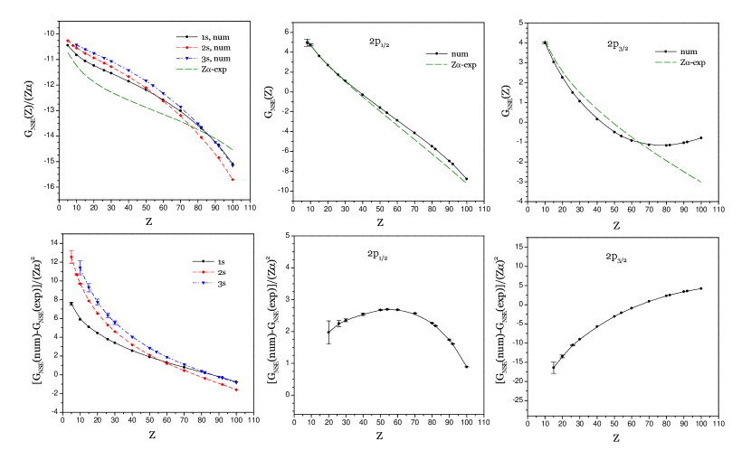
Comparison of the present numerical data for the function $G_{\rm NSE}$ with the ${Z\alpha}$-expansion results is given in three upper graphs of Fig. 1. Note that for $ns$ states, the ratio $G_{\rm NSE}({Z\alpha})/({Z\alpha})$ is plotted. The lower graphs in Fig. 1 depict the higher-order remainder (i.e., the contribution beyond the known terms of the ${Z\alpha}$ expansion). For $ns$ states, the remainder does not approach a finite limit as $Z\to 0$ because it contains $\ln({Z\alpha})$, as can be seen from Eqs. (II) and (11).
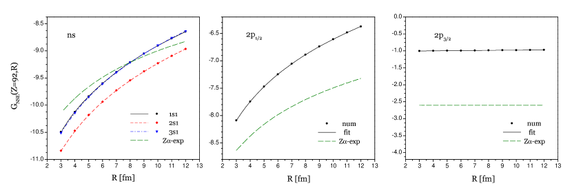
In Fig. 2, the dependence of $G_{\rm NSE}$ on the rms nuclear charge radius $R$ is studied, with the nuclear charge number fixed by $Z=92$. We find that the $R$ dependence of our numerical data can be well approximated by a three-parameter fit that includes $\ln R$, as suggested by the ${Z\alpha}$ expansion. More specifically, the following fitting functions approximate the numerical data for $Z=92$ in the region $R=3$–12 fm with the relative accuracy of better than $2\times 10^{-4}$ (with $R$ expressed in fermi units),

$\displaystyle G_{\rm NSE}(R;1s)=-11.8768+1.2083\,\ln R+0.0191\,R\,,$ (12)
$\displaystyle G_{\rm NSE}(R;2s)=-12.2394+1.2124\,\ln R+0.0220\,R\,,$ (13)
$\displaystyle G_{\rm NSE}(R;3s)=-11.9131+1.2143\,\ln R+0.0218\,R\,,$ (14)
$\displaystyle G_{\rm NSE}(R;2p_{1/2})=-9.4115+1.1759\,\ln R+0.0098\,R\,,$ (15)
$\displaystyle G_{\rm NSE}(R;2p_{3/2})=-1.0145+0.0019\,\ln R+0.0033\,R\,.$ (16)

III NS correction to vacuum polarization

The one-loop vacuum-polarization correction to the energy levels is usually represented as a sum of two parts, the Uehling and the Wichmann-Kroll ones mohr:98 . The Uehling part of the vacuum polarization is given by the expectation value of the potential

$\displaystyle U_{\rm Ueh}(r)$ $\displaystyle\ =-\frac{2\alpha^{2}Z}{3mr}\,\int_{0}^{\infty}dr^{\prime}r^{\prime}\rho(r^{\prime})\,$
$\displaystyle\times\left[K_{0}(2m|r-r^{\prime}|)-K_{0}(2m|r+r^{\prime}|)\right]\,,$ (17)

where

$$K_{0}(x)=\int_{1}^{\infty}dt\,e^{-xt}\left(\frac{1}{t^{3}}+\frac{1}{2t^{5}}\right)\,\sqrt{t^{2}-1}\,,$$ (18)

and the nuclear-charge density $\rho$ is normalized by the condition $\int d\bm{r}\,\rho(r)=1$. The energy shift due to the Wichmann-Kroll part of the vacuum polarization can be written as soff:88:vp ; manakov:89:zhetp

$\displaystyle\Delta E_{\rm WK}=$ $\displaystyle\,\frac{2\alpha}{\pi}\,{\rm Re}\,\sum_{\kappa}|\kappa|\,\int_{0}^{\infty}d\omega\,\int_{0}^{\infty}r^{2}dr\,\left(g_{a}^{2}+f_{a}^{2}\right)\,$
$\displaystyle\times\int_{r}^{\infty}dr^{\prime}r^{\prime}\,\left(1-\frac{r^{\prime}}{r}\right)\,{\rm Tr}\,G_{\kappa}^{(2+)}(i\omega,r^{\prime},r^{\prime})\,,$ (19)

where $g_{a}$ and $f_{a}$ are the upper and the lower radial components of the reference-state wave function, $G_{\kappa}^{(2+)}$ is the radial Dirac Green function that contains two and more interactions with the binding field,

$\displaystyle G^{(2+)}_{\kappa}(\omega,x,y)=\int_{0}^{\infty}$ $\displaystyle\,dz\,z^{2}\,G^{(0)}_{\kappa}(\omega,x,z)\,V(z)\,$
$\displaystyle\times$ $\displaystyle\ \left[G_{\kappa}(\omega,z,y)-G^{(0)}_{\kappa}(\omega,z,y)\right]\,,$ (20)

$G_{\kappa}$ is the radial part of the full Dirac Green function, $G^{(0)}_{\kappa}$ is the free Dirac Green function, and $V(z)$ is the binding potential. We note that Eq. (III) is valid both for the point-nucleus and the extended-nucleus binding potentials.

Calculations of the Wichmann-Kroll part of the one-loop vacuum polarization were extensively discussed in the literature over past decades soff:88:vp ; manakov:89:zhetp ; persson:93:vp ; sapirstein:03:vp . In the present work, we perform calculations of the vacuum polarization, evaluating the integrations and the summation over $\kappa$ in the order specified by Eqs. (III) and (III). Comparison of the numerical results obtained in this work for the Wichmann-Kroll correction with those reported in previous calculations persson:93:vp ; mohr:98 is presented in Table Acknowledgments.

The nuclear-size vacuum-polarization (NVP) correction is defined as the difference between the one-loop vacuum-polarization corrections evaluated with the point-Coulomb potential and the potential of the extended-charge nucleus. The NVP correction can be parameterized in the same way as the one-loop radiative corrections,

$\displaystyle\Delta E_{\rm NVP}=\frac{\alpha}{\pi}\,\frac{({Z\alpha})^{4}}{n^{3}}\,F_{\rm NVP}({Z\alpha},R)\,.$ (21)

The results of our numerical evaluation of the NVP correction for the $1s$, $2s$, $3s$, $2p_{1/2}$, and $2p_{3/2}$ states of H-like ions are presented in TableAcknowledgments. The calculation is performed for the Fermi model of the nuclear charge distribution. It is interesting to note that for the $2p_{3/2}$ state and high nuclear charges, the correction coming from the Wichmann-Kroll part of the vacuum polarization dominates over the Uehling part.

The leading dependence of the NVP correction on $R$ and ${Z\alpha}$ can be conveniently factorized out in terms of the first-order NS contribution $\Delta E_{\rm N}$ milstein:02:prl ; milstein:04 ,

$\displaystyle\Delta E_{\rm NVP}(njl)=\Delta E_{\rm N}(n\nicefrac{{1}}{{2}}l)\,\frac{\alpha}{\pi}\,{G}_{\rm NVP}(njl)\,.$ (22)

Note that similarly to the NSE correction, for the $np_{3/2}$ reference state, Eq. (22) has the first-order NS correction for the $np_{1/2}$ state as a prefactor.

The ${Z\alpha}$ expansion of the function ${G}_{\rm NVP}$ is given by

$\displaystyle{G}_{\rm NVP}(ns)=$ $\displaystyle\,({Z\alpha})\,a_{10}+({Z\alpha})^{2}\,\biggl{[}\frac{2}{3\gamma}\,\ln^{2}\frac{b}{R_{\rm sph}}$
$\displaystyle+a_{21}\,\ln({Z\alpha})^{-2}+f({Z\alpha},R_{\rm sph})+O(1)\biggr{]}\,,$ (23)
$\displaystyle{G}_{\rm NVP}(np_{j})=$ $\displaystyle\,a_{00}+({Z\alpha})\,a_{10}+({Z\alpha})^{2}\,\biggl{[}\frac{2}{3\gamma}\,\delta_{j,\nicefrac{{1}}{{2}}}\,\ln^{2}\frac{b}{R_{\rm sph}}$
$\displaystyle+\delta_{j,\nicefrac{{1}}{{2}}}\,f({Z\alpha},R_{\rm sph})+O(1)\biggr{]}\,,$ (24)

where $b=\exp[1/(2\gamma)-C-5/6]$, $\gamma=\sqrt{1-({Z\alpha})^{2}}$, and $C$ is the Euler constant. The leading term of the expansion for the $s$ states was calculated long ago friar:79 ; hylton:85 . All other coefficients except $a_{21}$ were derived in Refs. milstein:03:fns ; milstein:04 . The logarithmic $a_{21}$ term was pointed out by Pachucki pachucki:priv ; the value of the coefficient is the same as for the vacuum-polarization correction to the hyperfine splitting. The results for the expansion coefficients are

$\displaystyle a_{00}(np_{1/2})=a_{00}(np_{3/2})=-\nicefrac{{8}}{{45}}\,,$ (25)
$\displaystyle a_{10}(ns)=\nicefrac{{3\pi}}{{4}}\,,\ \ a_{10}(np_{1/2})=\nicefrac{{23\pi}}{{72}}\,,\ \ a_{10}(np_{3/2})=\nicefrac{{5\pi}}{{72}}\,,$ (26)
$\displaystyle a_{21}(ns)=\nicefrac{{4}}{{15}}\,,$ (27)

and milstein:04

$\displaystyle f({Z\alpha},R_{\rm sph})=$ $\displaystyle\ \frac{1}{3({Z\alpha})^{2}}\biggl{[}-2\ln R_{\rm sph}-\frac{5}{3}+\pi\tan(\pi\gamma)$
$\displaystyle+\frac{2}{3+2\gamma}+2\psi(-1-2\gamma)$
$\displaystyle-\frac{\pi^{3/2}(3+2\gamma)\Gamma(\gamma+1)}{40\sin(2\pi\gamma)(\gamma-1)\Gamma(-1-2\gamma)\Gamma(\gamma+3/2)}\,$
$\displaystyle\times\left(2R_{\rm sph}\right)^{2(1-\gamma)}\biggr{]}\,.$ (28)

The function $f({Z\alpha},R_{\rm sph})$ has a finite limit as ${Z\alpha}\to 0$, which is

$\displaystyle f(0,R_{\rm sph})=$ $\displaystyle\,\frac{1}{3}\,\ln^{2}R_{\rm sph}+\left(-\frac{4}{5}+\frac{2}{3}\,C\right)\,\ln R_{\rm sph}$
$\displaystyle+\frac{1}{3}\left(\frac{833}{255}-\frac{12}{5}\,C+C^{2}-\frac{\pi^{2}}{12}\right)\,.$ (29)

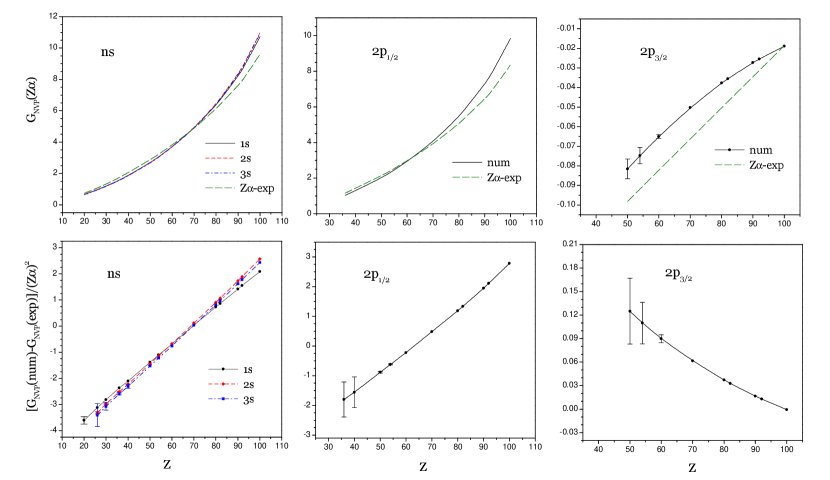
In Fig. 3, we compare the present numerical data for the function $G_{\rm NVP}$ with the ${Z\alpha}$-expansion results summarized above. We observe good agreement in all cases; the higher-order remainder function exhibits a nearly linear dependence on the nuclear charge number.

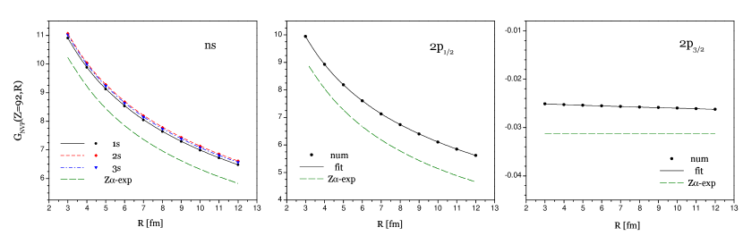
In Fig. 4, we study the dependence of the function $G_{\rm NVP}$ on the rms nuclear charge radius $R$, with the nuclear charge number fixed by $Z=92$. Similarly to the NSE correction, we find that the $R$ dependence of our numerical data can be well approximated by a three-parameter fit, whose form is suggested by the ${Z\alpha}$ expansion. More specifically, the following fitting functions approximate the numerical data for $Z=92$ in the region $R=3$–12 fm with the relative accuracy of better than $2\times 10^{-4}$ (with $R$ expressed in fermi units),

$\displaystyle G_{\rm NVP}(R;1s)=15.3607+0.3459\,\ln^{2}R-4.4325\,\ln R\,,$ (30)
$\displaystyle G_{\rm NVP}(R;2s)=15.5292+0.3397\,\ln^{2}R-4.4307\,\ln R\,,$ (31)
$\displaystyle G_{\rm NVP}(R;3s)=15.4820+0.3396\,\ln^{2}R-4.4321\,\ln R\,,$ (32)
$\displaystyle G_{\rm NVP}(R;2p_{1/2})=14.3668+0.3673\,\ln^{2}R-4.4346\,\ln R\,,$ (33)
$\displaystyle G_{\rm NVP}(R;2p_{3/2})=-0.02474-0.000134\,R+0.000001\,R^{2}\,.$ (34)

IV Results for hydrogen

In this section, we obtain all-order (in ${Z\alpha}$) results for the radiative nuclear size effect to the ground-state Lamb shift in hydrogen. This task is complicated by the fact that we are not able to perform calculations of the self-energy and Wichmann-Kroll parts of the nuclear size effect directly for $Z=1$. In the absence of a direct calculation, we perform extrapolation of the numerical data obtained for higher values of $Z$ to $Z=1$.

We start with the self energy. The data for the function $G_{\rm NSE}(Z,R)$ plotted in Fig. 1 is not well suited for extrapolation since individual points correspond to different values of the rms radius. Because of this, we repeat our calculations for different nuclear charges and the rms radius fixed by $R=r_{p}$, where $r_{p}=0.8768(69)$ fm is the CODATA value of the proton charge radius mohr:08:rmp . We also account for the fact that the Fermi model of the nuclear charge distribution is not completely adequate for small rms radii; the Gaussian model is employed instead, with $\rho(r)=\rho_{0}\,\exp(-\Lambda r^{2})$. The extrapolation is performed for the higher-order remainder function,

$${\cal G}^{\rm h.o.}_{\rm NSE}=[G_{\rm NSE}({\rm num})-G_{\rm NSE}({\rm ana})]/({Z\alpha})\,,$$ (35)

where $G_{\rm NSE}({\rm num})$ and $G_{\rm NSE}({\rm ana})$ denote the numerical and analytical [Eq. (II)] values of the $G_{\rm NSE}$ function. In our extrapolation, we used 20 points with the nuclear charges in the interval $Z=5-30$ and the same extrapolation procedure as in Ref. yerokhin:05:hfs . Our result for hydrogen is ${\cal G}^{\rm h.o.}_{\rm NSE}(Z=1)=0.075(25)$.

The Uehling part of the NVP correction is calculated directly, with the result (for the Gaussian model) $G_{\rm NVP,Ue}(Z=1)=2.5835\,\alpha$. The Wichmann-Kroll part is a small correction for hydrogen, its leading contribution to $G_{\rm NVP}$ being a constant term of order $({Z\alpha})^{2}$. Similarly to the NSE correction, we obtain the result for hydrogen by extrapolation. The data to be extrapolated is obtained by repeating our calculations for $Z=20-75$, with the rms radius fixed by $R=r_{p}$ and the nuclear charge distribution given by the Gaussian model. The extrapolation is performed for the ratio $G_{\rm NVP,WK}/({Z\alpha})^{2}$. The result for hydrogen is $G_{\rm NVP,WK}(Z=1)=-9.8(9)\,\alpha^{2}$.

Summarising our calculations of the radiative nuclear size effect to the $1s$ Lamb shift in hydrogen, we express the results in the same form as in Ref. mohr:08:rmp ,

$\displaystyle\Delta E_{\rm NSE}=\alpha^{2}Z\,{\cal E}_{\rm N}\,\bigl{[}-3.1294(80)\bigr{]}\,,$ (36)
$\displaystyle\Delta E_{\rm NVP}=\alpha^{2}Z\,{\cal E}_{\rm N}\,\bigl{[}0.8228-0.0228(23)\bigr{]}\,,$ (37)

where ${\cal E}_{\rm N}=2/3\,({Z\alpha})^{4}\,R^{2}$ and the first and the second terms in the brackets in Eq. (37) correspond to the Uehling and Wichmann-Kroll parts. In order to estimate the model dependence of our results, we evaluated the Uehling part also within the exponential model, with $\rho(r)=\rho_{0}\,\exp(-\Lambda\,r)$, and found a 0.2% deviation from the Gaussian result.

The numerical constant terms in Eqs. (36) and (37) can be compared with the ${Z\alpha}$-expansion results. For the self-energy, the leading-order term of the ${Z\alpha}$ expansion is $4\ln 2-\nicefrac{{23}}{{4}}=-2.977$, whereas all terms in Eq. (II) yield the coefficient of $-3.153$. For the vacuum polarization, the leading-order term is $\nicefrac{{3}}{{4}}$, whereas all terms in Eq. (III) yield $0.827$. We conclude that the higher-order corrections increase the leading-order result for the radiative nuclear size effect in hydrogen by 4.4%.

Conclusion

In the present investigation, we evaluate the nuclear size correction to the Lamb shift of the $1s$, $2s$, $3s$, $2p_{1/2}$, and $2p_{3/2}$ states of hydrogen-like atoms. The treatment is complete at the one-loop level, i.e., it includes the leading-order effect as well as the one-loop radiative corrections. The total nuclear size correction to the energy level is represented, for the $ns$ and $np_{1/2}$ states, as

$\displaystyle\Delta E_{\rm NS}=\Delta E_{\rm N}\,\biggl{[}1+\frac{\alpha}{\pi}\,\left(G_{\rm NSE}+G_{\rm NVP}\right)\biggr{]}\,,$ (38)

and, for the $np_{3/2}$ states, as

$\displaystyle\Delta E_{\rm NS}(np_{3/2})=$ $\displaystyle\,\Delta E_{\rm N}(np_{3/2})$
$\displaystyle+\Delta E_{\rm N}(np_{1/2})\,\frac{\alpha}{\pi}\,\left(G_{\rm NSE}+G_{\rm NVP}\right)\,,$ (39)

where $\Delta E_{\rm N}$ is the nuclear size correction to the Dirac energy. The all-order numerical values obtained for the self-energy and vacuum-polarization functions $G_{\rm NSE}$ and $G_{\rm NVP}$ were compared with results of the ${Z\alpha}$-expansion calculations. Inclusion of the logarithmic term of the relative order $({Z\alpha})^{2}\ln^{2}({Z\alpha})^{-2}$ for $ns$ states was necessary in order to achieve agreement between different calculations. Extrapolation of the all-order data obtained for hydrogen-like ions to $Z=1$ provides an all-order result for the radiative nuclear size effect on the ground-state Lamb shift in hyrogen. The higher-order corrections are shown to increase the leading-order result by 4.4%.

Acknowledgments

I wish to thank Krzysztof Pachucki for valuable comments and advices. Computations reported in this work were performed on the computer cluster of St. Petersburg State Polytechnical University.

Table 1: Nuclear-size correction to the Dirac energies of H-like ions, in terms of the function $G_{\rm N}({Z\alpha},R)$ defined by Eq. (4). Fermi model of the nuclear charge distribution is used.
$Z$ $R$ [fm] $1s$ $2s$ $3s$ $2p_{1/2}$
5 2.4059 $1.000\,46$ $1.000\,71$ $1.000\,23$ $1.001\,73$
8 2.7013 $1.003\,91$ $1.004\,55$ $1.003\,33$ $1.006\,89$
10 3.0053 $1.006\,57$ $1.007\,58$ $1.005\,67$ $1.011\,17$
15 3.1888 $1.015\,66$ $1.017\,93$ $1.013\,60$ $1.025\,66$
20 3.4764 $1.028\,67$ $1.032\,74$ $1.024\,91$ $1.046\,42$
26 3.7371 $1.049\,77$ $1.056\,75$ $1.043\,18$ $1.080\,18$
30 3.9286 $1.067\,32$ $1.076\,73$ $1.058\,28$ $1.108\,52$
40 4.2696 $1.124\,66$ $1.142\,02$ $1.106\,96$ $1.202\,64$
50 4.6543 $1.203\,59$ $1.232\,01$ $1.172\,31$ $1.337\,09$
60 4.9118 $1.308\,62$ $1.351\,81$ $1.256\,25$ $1.524\,64$
70 5.3115 $1.445\,02$ $1.507\,15$ $1.359\,74$ $1.784\,78$
82 5.5010 $1.662\,15$ $1.752\,74$ $1.511\,54$ $2.236\,31$
92 5.8569 $1.896\,75$ $2.013\,31$ $1.655\,09$ $2.785\,73$
100 5.8570 $2.128\,53$ $2.263\,06$ $1.774\,54$ $3.393\,88$
Table 2: Different calculations of the nuclear-size self-energy correction to the energy levels of H-like ions, in terms of the function $F_{\rm NSE}({Z\alpha},R)$ defined by Eq. (8), for the homogeneously charged sphere model.
$Z$ $R$ [fm] $1s$ $2s$ $2p_{1/2}$ Ref.
26 3.730 $-0.000\,172\,122(4)$ $-0.000\,173\,29(1)$ $0.000\,000\,972(2)$
$-0.000\,172(1)$ $-0.000\,18(1)$ $-0.000\,00(1)$ mohr:93:prl
54 4.826 $-0.001\,274\,870(2)$ $-0.001\,461\,69(1)$ $-0.000\,020\,391(2)$
$-0.001\,275(1)$ $-0.001\,462(1)$ $-0.000\,021(1)$ mohr:93:prl
92 5.863 $-0.018\,491\,8(8)$ $-0.029\,089\,3(9)$ $-0.002\,482\,76(8)$
$-0.018\,492(1)$ $-0.029\,090(2)$ $-0.002\,483(1)$ mohr:93:prl
Table 3: Nuclear-size self-energy correction to the energy levels of H-like ions, in terms of the function $F_{\rm NSE}({Z\alpha},R)$ defined by Eq. (8). Fermi model of the nuclear charge distribution is used. The nuclear charge rms radii used are listed in Table Acknowledgments.
$Z$ $1s$ $2s$ $3s$ $2p_{1/2}$ $2p_{3/2}$
5 $-0.000\,009\,962(6)$ $-0.000\,009\,81(2)$ $\,$ $\,$ $\,$
8 $-0.000\,020\,969(2)$ $-0.000\,020\,53(1)$ $\,$ $0.000\,000\,107(8)$ $\,$
10 $-0.000\,033\,242(2)$ $-0.000\,032\,54(1)$ $-0.000\,032\,12(3)$ $0.000\,000\,201(4)$ $0.000\,000\,170(2)$
15 $-0.000\,060\,128(2)$ $-0.000\,059\,10(1)$ $-0.000\,058\,21(4)$ $0.000\,000\,412(2)$ $0.000\,000\,345(2)$
20 $-0.000\,102\,940(2)$ $-0.000\,102\,06(2)$ $-0.000\,100\,38(2)$ $0.000\,000\,699(2)$ $0.000\,000\,587(2)$
26 $-0.000\,172\,537(2)$ $-0.000\,173\,71(3)$ $-0.000\,170\,72(3)$ $0.000\,000\,976(2)$ $0.000\,000\,852(2)$
30 $-0.000\,238\,936(2)$ $-0.000\,243\,68(3)$ $-0.000\,239\,45(3)$ $0.000\,001\,021(2)$ $0.000\,000\,969(2)$
40 $-0.000\,481\,097(2)$ $-0.000\,511\,07(2)$ $-0.000\,502\,4(1)$ $-0.000\,000\,726(2)$ $0.000\,000\,396(2)$
50 $-0.000\,960\,607(2)$ $-0.001\,075\,22(2)$ $-0.001\,057\,8(1)$ $-0.000\,010\,544(2)$ $-0.000\,003\,299(2)$
60 $-0.001\,830\,75(1)$ $-0.002\,183\,28(2)$ $-0.002\,150\,3(4)$ $-0.000\,046\,025(4)$ $-0.000\,014\,862(2)$
70 $-0.003\,730\,19(4)$ $-0.004\,791\,85(6)$ $-0.004\,722\,0(2)$ $-0.000\,170\,450(6)$ $-0.000\,047\,078(2)$
82 $-0.008\,404\,0(2)$ $-0.011\,977\,2(2)$ $-0.011\,796\,6(4)$ $-0.000\,703\,91(2)$ $-0.000\,140\,462(2)$
92 $-0.018\,426\,6(7)$ $-0.028\,986\,6(8)$ $-0.028\,474\,0(6)$ $-0.002\,473\,96(6)$ $-0.000\,337\,183(2)$
100 $-0.034\,060(2)$ $-0.058\,444(3)$ $-0.057\,172(1)$ $-0.006\,696\,3(4)$ $-0.000\,602\,404(2)$
Table 4: Coefficients of the ${Z\alpha}$ expansion of the NSE correction in Eq. (II).
Term State Value Ref.
$a_{01}$ $np_{j}$ $\nicefrac{{8}}{{9}}$ milstein:03:fns ; jentschura:03:jpa
$a_{00}$ $2p_{1/2}$ 0.808 879 967(1) milstein:03:fns ; jentschura:03:jpa
$np_{3/2}$ $a_{00}(np_{1/2})-1$ milstein:03:fns ; jentschura:03:jpa
$a_{10}$ $ns$ $\pi\left(-\nicefrac{{23}}{{4}}+4\ln 2\right)$ pachucki:93:density ; eides:97:pra ; milstein:02:prl
$np_{1/2}$ $\pi\left(\nicefrac{{379}}{{432}}-\nicefrac{{16}}{{3}}\ln 2\right)$ milstein:04
$np_{3/2}$ $\pi\left(\nicefrac{{559}}{{432}}-4\ln 2\right)$ milstein:04
$a_{\log}$ $ns$, $np_{1/2}$ $\nicefrac{{\pi^{2}}}{{6}}-\nicefrac{{15}}{{4}}$ milstein:02:prl ; milstein:03:fns
$a_{22}$ $ns$ $-\nicefrac{{2}}{{3}}$ pachucki:priv
$a_{21}$ $np_{1/2}$ $-2(n^{2}-1)/n^{2}$ pachucki:priv ; jentschura:10

Refer to caption

Figure 1: (Color online) Nuclear-size self-energy correction, in terms of $G_{\rm NSE}$ defined by Eq. (9), as a function of the nuclear charge number $Z$. The upper graphs depict the ratio $G_{\rm NSE}(Z)/({Z\alpha})$ for the $ns$ states and the function $G_{\rm NSE}(Z)$ for the $np_{j}$ states, in comparison with the ${Z\alpha}$-expansion results. The lower graphs show the difference between the all-order and ${Z\alpha}$-expansion results for the function $G_{\rm NSE}$ divided by $({Z\alpha})^{2}$.

Refer to caption

Figure 2: (Color online) Nuclear-size self-energy correction, in terms of $G_{\rm NSE}({Z\alpha},R)$ defined by Eq. (9), as a function of the rms nuclear charge radius $R$, for $Z=92$.
Table 5: Different calculations of the Wichmann-Kroll vacuum-polarization correction [Eq. (III)] to the energy levels of H-like ions, in units $\Delta E/[(\alpha/\pi)\,({Z\alpha})^{4}/n^{3}]$.
$Z$ $R$ [fm] Model $1s$ $2s$ $2p_{1/2}$ $2p_{3/2}$ Ref.
36 4.230 sphere $0.002\,741\,99(6)$ $0.002\,833\,98(3)$ $0.000\,083\,36(4)$ $0.000\,027\,95(4)$
sphere $0.002\,741\,8$ $0.002\,833\,7$ $0.000\,083\,4$ $0.000\,028\,0$ persson:93:vp
shell $0.002\,7$ $0.002\,8$ $0.000\,1$ $0.000\,0$ mohr:98
54 4.826 sphere $0.005\,921\,2(2)$ $0.006\,423\,4(2)$ $0.000\,454\,79(2)$ $0.000\,114\,18(5)$
sphere $0.005\,921\,1$ $0.006\,423\,1$ $0.000\,454\,8$ $0.000\,114\,2$ persson:93:vp
shell $0.005\,9$ $0.006\,4$ $0.000\,4$ $0.000\,1$ mohr:98
92 5.860 sphere $0.020\,679\,2(5)$ $0.027\,252\,0(8)$ $0.006\,824\,1(4)$ $0.000\,749\,49(6)$
sphere $0.020\,678\,9$ $0.027\,251\,5$ $0.006\,824\,0$ $0.000\,749\,4$ persson:93:vp
shell $0.020\,6$ $0.027\,2$ $0.006\,8$ $0.000\,7$ mohr:98
Table 6: Nuclear-size vacuum-polarization correction to the energy levels of H-like ions, in terms of the function $F_{\rm NVP}({Z\alpha},R)$ defined by Eq. (21). Fermi model of the nuclear charge distribution is used. The nuclear charge rms radii used are listed in Table Acknowledgments. For a given $Z$, the upper line (“Ue”) corresponds to the Uehling part and the lower line (“WK”), to the Wichmann-Kroll part.
$Z$ $1s$ $2s$ $3s$ $2p_{1/2}$ $2p_{3/2}$
15 Ue $0.000\,024\,856$ $0.000\,024\,968$ $0.000\,024\,921$ $0.000\,000\,020$ $-0.000\,000\,016$
20 Ue $0.000\,047\,62$ $0.000\,048\,21$ $0.000\,048\,12$ $0.000\,000\,102$ $-0.000\,000\,034$
WK $-0.000\,006\,4(2)$ $-0.000\,006(1)$ $-0.000\,006(3)$ $\,$ $\,$
26 Ue $0.000\,089\,44$ $0.000\,091\,72$ $0.000\,091\,60$ $0.000\,000\,402$ $-0.000\,000\,064$
WK $-0.000\,012\,58(1)$ $-0.000\,012\,9(1)$ $-0.000\,013(1)$ $\,$ $\,$
30 Ue $0.000\,131\,907(2)$ $0.000\,136\,725(2)$ $0.000\,136\,601(2)$ $0.000\,000\,865$ $-0.000\,000\,092$
WK $-0.000\,018\,83(3)$ $-0.000\,019\,55(9)$ $-0.000\,019\,6(7)$ $\,$ $\,$
40 Ue $0.000\,304\,304(4)$ $0.000\,326\,352(4)$ $0.000\,326\,510(4)$ $0.000\,004\,205$ $-0.000\,000\,188$
WK $-0.000\,043\,43(4)$ $-0.000\,046\,5(1)$ $-0.000\,046\,6(9)$ $-0.000\,000\,9(1)$ $\,$
50 Ue $0.000\,674\,503(2)$ $0.000\,756\,416(2)$ $0.000\,758\,099(2)$ $0.000\,016\,672$ $-0.000\,000\,342$
WK $-0.000\,092\,38(7)$ $-0.000\,102\,71(7)$ $-0.000\,103\,07(9)$ $-0.000\,003\,37(2)$ $-0.000\,000\,20(2)$
60 Ue $0.001\,410\,95(1)$ $0.001\,673\,01(1)$ $0.001\,680\,03(1)$ $0.000\,057\,40$ $-0.000\,000\,546$
WK $-0.000\,181\,6(2)$ $-0.000\,211\,8(3)$ $-0.000\,212\,8(3)$ $-0.000\,010\,46(2)$ $-0.000\,000\,49(2)$
70 Ue $0.003\,100\,32(1)$ $0.003\,932\,42(2)$ $0.003\,956\,23(2)$ $0.000\,197\,79$ $-0.000\,000\,872$
WK $-0.000\,367\,7(4)$ $-0.000\,454\,6(5)$ $-0.000\,456\,8(5)$ $-0.000\,032\,06(4)$ $-0.000\,001\,201(4)$
82 Ue $0.007\,710\,07(4)$ $0.010\,779\,92(6)$ $0.010\,863\,65(6)$ $0.000\,822\,122(5)$ $-0.000\,001\,310$
WK $-0.000\,821\,5(7)$ $-0.001\,106\,2(9)$ $-0.001\,111\,4(9)$ $-0.000\,114\,34(9)$ $-0.000\,003\,021(4)$
92 Ue $0.018\,230\,65$ $0.028\,056\,439(2)$ $0.028\,275\,306(4)$ $0.002\,970\,972$ $-0.000\,001\,923$
WK $-0.001\,762\,6(8)$ $-0.002\,587(1)$ $-0.002\,594(1)$ $-0.000\,361\,0(2)$ $-0.000\,006\,750(3)$
100 Ue $0.036\,429\,910(6)$ $0.061\,165\,53(1)$ $0.061\,549\,11(1)$ $0.008\,427\,011(2)$ $-0.000\,002\,344$
WK $-0.003\,259(2)$ $-0.005\,184(4)$ $-0.005\,183(4)$ $-0.000\,915\,4(6)$ $-0.000\,012\,100(6)$

Refer to caption

Figure 3: (Color online) Nuclear-size vacuum-polarization correction, in terms of $G_{\rm NVP}({Z\alpha},R)$ defined by Eq. (21), as a function of the nuclear charge number $Z$.

Refer to caption

Figure 4: (Color online) Nuclear-size vacuum-polarization correction, in terms of $G_{\rm NVP}({Z\alpha},R)$ defined by Eq. (21), as a function of the rms nuclear charge radius $R$, for $Z=92$.

Appendix A Dirac Green function for a general potential

In this section we construct the Green function of the Dirac equation with the potential $V(r)$ of a general form. We assume that the potential $V(r)$ differs from the Coulomb one within a finite (inner) region only, i.e., there is $r_{0}$ such that, for $r>r_{0}$, $V(r)=-Z\alpha/r$, with $Z\geq 0$. For our purposes, it is sufficient to consider the potential to be regular at the origin, i.e., $rV(r)\to 0$ as $r\to 0$. In the inner region $r<r_{0}$, the combination $rV(r)$ is assumed to be well represented by a piecewise cubic polynomial calculated on a sufficiently dense grid.

The radial Dirac Green function $G_{\kappa}(E,r_{1},r_{2})$ is expressed in terms of the two-component solutions of the radial Dirac equation regular at the origin $\left(\phi_{\kappa}^{0}\right)$ and the infinity $\left(\phi_{\kappa}^{\infty}\right)$ as follows

$\displaystyle G_{\kappa}(E,r_{1},r_{2})=$ $\displaystyle\,-\phi_{\kappa}^{\infty}(E,r_{1})\,\phi_{\kappa}^{0^{T}}(E,r_{2})\,\theta(r_{1}-r_{2})$
$\displaystyle-\phi_{\kappa}^{0}(E,r_{1})\,\phi_{\kappa}^{{\infty}^{T}}(E,r_{2})\,\theta(r_{2}-r_{1})\,.$ (40)

The solutions are normalized by the condition that their Wronskian is unity (everywhere except for the bound-state energies),

$\displaystyle\phi_{\kappa}^{0^{T}}(E,r)\left(\begin{array}[]{cc}0&-1\\ 1&0\\ \end{array}\right)\phi_{\kappa}^{\infty}(E,r)=1\,.$ (43)

In the present work, we obtain the radial solutions in the inner region $r<r_{0}$ by a numerical solution of the Dirac equation on a grid, whereas in the outer region $r>r_{0}$, we express them as a combination of the radial solutions of the Dirac-Coulomb problem. The regular and irregular solutions of the Dirac equation with the point-nucleus Coulomb potential will be denoted by $\psi_{\kappa}^{0}$ and $\psi_{\kappa}^{\infty}$, respectively. They are known analytically in terms of the Whittaker functions, see e.g., Ref. mohr:98 . (Note the sign difference of the present definition of the Green function as compared to that of Ref. mohr:98 .) In this work, the Dirac-Coulomb solutions $\psi_{\kappa}^{0}$ and $\psi_{\kappa}^{\infty}$ are evaluated by a generalization of the procedure described in Ref. yerokhin:99:pra .

The general calculational scheme is as follows. For a given energy argument $E$, we calculate and store the solutions $\psi_{\kappa}^{0}$ and $\psi_{\kappa}^{\infty}$ on a radial grid $\left\{r_{i}\right\}_{i=1}^{N}$ and then obtain the radial Green function for arbitrary radial arguments by interpolation. Large number of the mesh points ($N\sim 10^{4}$) and a careful choice of the grid allow us to minimize losses of accuracy due to interpolation. In order to avoid numerical overflow (underflow) when storing the regular and irregular solutions for large imaginary energies $E$ and large $\kappa$, all manipulations are performed with the “normalized” solutions in which the approximate large-$r$ and small-$r$ behaviour is pulled out,

$\displaystyle\widetilde{\phi}_{\kappa}^{0}(E,r)=r^{-|\kappa|}\,e^{-cr}\,\phi_{\kappa}^{0}(E,r)\,,$ (44)
$\displaystyle\widetilde{\phi}_{\kappa}^{\infty}(E,r)=r^{|\kappa|}\,e^{cr}\,\phi_{\kappa}^{\infty}(E,r)\,,$ (45)

where $c=\sqrt{1-E^{2}}$. Advantages of the normalized solutions are, first, that they are more suitable for interpolation than the original solutions and, more importantly, that they can be stored and manipulated within the standard double precision arithmetics (in the range of $\kappa$’s relevant for the present investigation, up to $|\kappa|\sim 30$).

In the inner region $r<r_{0}$, we calculate the regular solution $\phi_{\kappa}^{0}$ (or, rather, $\widetilde{\phi}_{\kappa}^{0}$) by solving the radial Dirac equation on a grid as described in the following, starting from $r=0$ and up to $r=r_{0}$. For $r>r_{0}$, the potential is the Coulomb one and the regular solution $\phi_{\kappa}^{0}$ is a linear combination of the regular and irregular Dirac-Coulomb solutions,

$\displaystyle\phi_{\kappa}^{0}(E,r)=a\,\psi_{\kappa}^{0}(E,r)+b\,\psi_{\kappa}^{\infty}(E,r)\,,\ \ \ r\geq r_{0}\,.$ (46)

The coefficients $a$ and $b$ are defined by the condition that the two components of $\phi_{\kappa}^{0}$ are continuous at $r=r_{0}$. So, we determine the coefficients $a$ and $b$ by matching the numerical and the analytical solutions at $r=r_{0}$ and employ the analytical Dirac-Coulomb functions for calculations for $r>r_{0}$.

The irregular solution $\phi_{\kappa}^{\infty}$ in the outer region is just the Dirac Coulomb function,

$\displaystyle\phi_{\kappa}^{\infty}(E,r)=\psi_{\kappa}^{\infty}(E,r)\,,\ \ \ r\geq r_{0}\,.$ (47)

So, we use the analytical representation for $r\geq r_{0}$. For smaller $r$, the irregular solution is calculated by solving the Dirac equation on a grid, downward from $r=r_{0}$ towards $r=0$. The normalization of the numerical solution is fixed by requiring continuity at the point $r=r_{0}$.

We now turn to the problem of solving the Dirac equation with the potential $V(r)$ on a grid. In this work, we employ the power series solution method, previously applied to the Dirac equation by Salvat et al. salvat:95:cpc . For completeness, we give here the description of the method. First, let us solve the equation on the interval $[r_{a},r_{b}]$ with given boundary conditions at $r=r_{a}$. The situation $r_{b}<r_{a}$ is allowed and it is assumed that $r_{a}>0$. (The special case of $r_{a}=0$ will be considered separately.) The radial Dirac equation is (with $m=1$)

$\displaystyle G^{\prime}(r)$ $\displaystyle\ =-\frac{\kappa}{r}\,G(r)+(E-V(r)+1)\,F(r)\,,$ (48)
$\displaystyle F^{\prime}(r)$ $\displaystyle\ =\frac{\kappa}{r}\,F(r)-(E-V(r)-1)\,G(r)\,,$ (49)

where $G(r)=rg(r)$ and $F(r)=rf(r)$ are the upper and lower components of the radial Dirac solution. Introducing new variables $x=(r-r_{a})/h$ and $h=r_{b}-r_{a}$, the equation is written as

$\displaystyle(xh+r_{a})G^{\prime}_{x}+\kappa hG+UhF-(xh+r_{a})hF$ $\displaystyle\ =0\,,$ (50)
$\displaystyle(xh+r_{a})F^{\prime}_{x}-\kappa hF-UhG-(xh+r_{a})hG$ $\displaystyle\ =0\,,$ (51)

where $U=r(V(r)-E)$. On the given interval, $U$ is represented by a cubic polynomial of $x$, $U=\sum_{k=0}^{3}u_{k}x^{k}$. The solutions are represented as power series of the form

$\displaystyle G(x)=\sum_{n=0}^{n_{\rm max}}a_{n}x^{n}\,,\ \ \ F(x)=\sum_{n=0}^{n_{\rm max}}b_{n}x^{n}\,,$ (52)

with the coefficients $a_{0}$ and $b_{0}$ determined by the boundary conditions $a_{0}=G(r_{a})$ and $b_{0}=F(r_{a})$. The coefficients $a_{n}$ and $b_{n}$ are determined by the recurrence relations (valid for $r_{a}\neq 0$)

$\displaystyle a_{n}$ $\displaystyle\ =-\frac{h}{nr_{a}}\bigl{[}(n-1+\kappa)a_{n-1}+(u_{0}-r_{a})b_{n-1}$
$\displaystyle+(u_{1}-h)b_{n-2}+u_{2}b_{n-3}+u_{3}b_{n-4}\bigr{]}\,,$ (53)
$\displaystyle b_{n}$ $\displaystyle\ =\frac{h}{nr_{a}}\bigl{[}(-n+1+\kappa)b_{n-1}+(u_{0}+r_{a})a_{n-1}$
$\displaystyle+(u_{1}+h)a_{n-2}+u_{2}a_{n-3}+u_{3}a_{n-4}\bigr{]}\,.$ (54)

The solutions at the end point are given by the sum of the coefficients,

$\displaystyle G(r_{b})=\sum_{n=0}^{n_{\rm max}}a_{n}\,,\ \ \ F(r_{b})=\sum_{n=0}^{n_{\rm max}}b_{n}\,.$ (55)

In the numerical evaluation, the recurrence relations are applied upwards until either the desired precision or the upper limit for $n$ (typically, $n_{\rm max}=30$) is reached. In the latter case, the interval is subdivided into two parts and the procedure is repeated until the desired accuracy is attained. This simple approach allows one to solve the equation with accuracy close to the machine precision.

Now, we consider the special case of $r_{a}=0$. In this case, the solutions are represented by the power expansion of the form

$\displaystyle G(x)=x^{s}\,\sum_{n=0}^{n_{\rm max}}a_{n}x^{n}\,,\ \ \ F(x)=x^{s+t}\,\sum_{n=0}^{n_{\rm max}}b_{n}x^{n}\,,$ (56)

where the parameters $s$ and $t$ are determined from the Dirac equation. For $\kappa<0$, we have (for the regular potentials considered here) $s=|\kappa|$ and $t=1$. The series start with

$\displaystyle a_{0}=1\,,\ \ \ b_{0}=\frac{h+u_{1}}{1+2|\kappa|}\,.$ (57)

The recursion relations take the form

$\displaystyle na_{n}=(u_{1}-h)b_{n-2}+u_{2}b_{n-3}+u_{3}b_{n-4}\,,$ (58)
$\displaystyle(2|\kappa|+n+1)b_{n}=(h+u_{1})a_{n}+u_{2}a_{n-1}+u_{3}a_{n-2}\,.$ (59)

For $\kappa>0$, one gets $s=\kappa+1$ and $t=-1$. The series start with

$\displaystyle a_{0}=\frac{h-u_{1}}{1+2\kappa}\,,\ \ \ b_{0}=1\,,$ (60)

whereas the recursion relations are

$\displaystyle(2\kappa+n+1)a_{n}=(h-u_{1})b_{n}-u_{2}b_{n-1}-u_{3}b_{n-2}\,,$ (61)
$\displaystyle nb_{n}=(u_{1}+h)a_{n-2}+u_{2}a_{n-3}+u_{3}a_{n-4}\,.$ (62)

Appendix B One-potential Dirac Green function for a general potential

For the evaluation of the self-energy correction, the one-potential Dirac Green function $G^{(1)}$ is needed. Its radial part is defined as

$\displaystyle G_{\kappa}^{(1)}(E,r_{1},r_{2})=\int_{0}^{\infty}dz\,z^{2}\,V(z)\,G^{(0)}_{\kappa}(E,r_{1},z)\,G^{(0)}_{\kappa}(E,z,r_{2})\,,$ (63)

where $G^{(0)}$ is the free Dirac Green function. Substituting the representation (A) for $G^{(0)}_{\kappa}$ into (63) and introducing the integral functions

$\displaystyle J_{\kappa}^{00}(r)=\int_{0}^{r}dz\,z^{2}\,V(z)\,\varphi^{0^{T}}_{\kappa}(z)\,\varphi^{0}_{\kappa}(z)\,,$ (64)
$\displaystyle J_{\kappa}^{i0}(r)=\int_{0}^{r}dz\,z^{2}\,V(z)\,\varphi^{{\infty}^{T}}_{\kappa}(z)\,\varphi^{0}_{\kappa}(z)\,,$ (65)
$\displaystyle J_{\kappa}^{ii}(r)=\int_{r}^{\infty}dz\,z^{2}\,V(z)\,\varphi^{{\infty}^{T}}_{\kappa}(z)\,\varphi^{\infty}_{\kappa}(z)\,,$ (66)

where $\varphi_{\kappa}^{(0)}$ $\left(\varphi_{\kappa}^{(\infty)}\right)$ denote the regular (irregular) solutions of the free Dirac equation, we write the one-potential Dirac Green function for $r_{1}\leq r_{2}$ as

$\displaystyle G_{\kappa}^{(1)}(E,r_{1},r_{2})=\Phi^{0}_{\kappa}(r_{1})\,\varphi_{\kappa}^{{\infty}^{T}}(r_{2})+\varphi^{0}_{\kappa}(r_{1})\,\Phi_{\kappa}^{{\infty}^{T}}(r_{2})\,,$ (67)

where

$\displaystyle\ \Phi^{0}_{\kappa}(r)=\varphi_{\kappa}^{\infty}(r)\,J_{\kappa}^{00}(r)-\varphi_{\kappa}^{0}(r)\,J_{\kappa}^{i0}(r)\,,$ (68)
$\displaystyle\ \Phi^{\infty}_{\kappa}(r)=\varphi_{\kappa}^{\infty}(r)\,J_{\kappa}^{i0}(r)+\varphi_{\kappa}^{0}(r)\,J_{\kappa}^{ii}(r)\,.$ (69)

For $r_{1}>r_{2}$, the one-potential Green function is obtained by the symmetry condition,

$\displaystyle G_{\kappa}^{(1)}(E,r_{1},r_{2})=G_{\kappa}^{{(1)}^{T}}(E,r_{2},r_{1})\,.$ (70)

Analogously to the approach used for the full Dirac Green function, we store the functions $\varphi_{\kappa}$ and $\Phi_{\kappa}$ on a radial grid $\left\{r_{i}\right\}_{i=1}^{N}$ and obtain the one-potential Green function by interpolation. The integral functions $J_{\kappa}$ are evaluated by numerical integration with help of Gauss-Legendre quadratures. The integration interval $(0,\infty)$ is breaked up at the position of the mesh points $r_{i}$, so that only one integral over $(0,\infty)$ needs to be evaluated for a given value of $E$. Analogously to the case of the full Green function, all manipulations with the regular and irregular solutions are carried out after normalizing them according to Eqs. (44) and (45), in order to prevent numerical overflow and underflow. Similar method of computation of the one-potential Green function was used long ago by M. Gyulassy in his evaluation of the vacuum-polarization gyulassy:75 .

References

  • (1) J. L. Friar, Z. Phys. A 292, 1 (1979), [ibid. 303, 84(E) (1981)].
  • (2) D. J. Hylton, Phys. Rev. A 32, 1303 (1985).
  • (3) K. Pachucki, Phys. Rev. A 48, 120 (1993).
  • (4) A. I. Milstein, O. P. Sushkov, and I. S. Terekhov, Phys. Rev. A 67, 062111 (2003).
  • (5) U. D. Jentschura, J. Phys. A 36, L229 (2003).
  • (6) A. I. Milstein, O. P. Sushkov, and I. S. Terekhov, Phys. Rev. A 69, 022114 (2004).
  • (7) G. Soff and P. Mohr, Phys. Rev. A 38, 5066 (1988).
  • (8) P. J. Mohr and G. Soff, Phys. Rev. Lett. 70, 158 (1993).
  • (9) R. Pohl et al., Nature (London) 466, 213 (2010).
  • (10) V. M. Shabaev, J. Phys. B 26, 1103 (1993).
  • (11) F. Salvat, J. M. Fernández-Varea, and W. Williamson Jr., Comput. Phys. Commun. 90, 151 (1995).
  • (12) V. M. Shabaev, I. I. Tupitsyn, V. A. Yerokhin, G. Plunien, and G. Soff, Phys. Rev. Lett. 93, 130405 (2004).
  • (13) I. Angeli, At. Data Nucl. Data Tables 87, 185 (2004).
  • (14) Y. S. Kozhedub, O. V. Andreev, V. M. Shabaev, I. I. Tupitsyn, C. Brandau, C. Kozhuharov, G. Plunien, and T. Stöhlker, Phys. Rev. A 77, 032501 (2008).
  • (15) P. J. Mohr, G. Plunien, and G. Soff, Phys. Rep. 293, 227 (1998).
  • (16) P. J. Mohr, Ann. Phys. (NY) 88, 26 (1974).
  • (17) S. A. Blundell and N. J. Snyderman, Phys. Rev. A 44, R1427 (1991).
  • (18) U. D. Jentschura, P. J. Mohr, and G. Soff, Phys. Rev. Lett. 82, 53 (1999).
  • (19) K. T. Cheng, W. R. Johnson, and J. Sapirstein, Phys. Rev. A 47, 1817 (1993).
  • (20) V. A. Yerokhin and V. M. Shabaev, Phys. Rev. A 60, 800 (1999).
  • (21) V. A. Yerokhin, K. Pachucki, and V. M. Shabaev, Phys. Rev. A 72, 042502 (2005).
  • (22) A. I. Milstein, O. P. Sushkov, and I. S. Terekhov, Phys. Rev. Lett. 89, 283003 (2002).
  • (23) K. Pachucki, private communication, 2010.
  • (24) N. L. Manakov, A. A. Nekipelov, and A. G. Fainshtein, Zh. Eksp. Teor. Fiz. 95, 1167 (1989), [Sov. Phys. JETP 68, 673 (1989)].
  • (25) H. Persson, I. Lindgren, S. Salomonson, and P. Sunnergren, Phys. Rev. A 48, 2772 (1993).
  • (26) J. Sapirstein and K. T. Cheng, Phys. Rev. A 68, 042111 (2003).
  • (27) P. J. Mohr, B. N. Taylor, and D. B. Newell, Rev. Mod. Phys. 80, 633 (2008).
  • (28) V. A. Yerokhin, A. N. Artemyev, V. M. Shabaev, and G. Plunien, Phys. Rev. A 72, 052510 (2005).
  • (29) M. I. Eides and H. Grotch, Phys. Rev. A 56, R2507 (1997).
  • (30) U. D. Jentschura and V. A. Yerokhin, Phys. Rev. A 81, 012503 (2010).
  • (31) M. Gyulassy, Nucl. Phys. A 244, 497 (1975).