Scaling of noise correlations in one-dimensional-lattice-hard-core-boson systems

Abstract

Noise correlations are studied for systems of hard-core bosons in one-dimensional lattices. We use an exact numerical approach based on the Bose-Fermi mapping and properties of Slater determinants. We focus on the scaling of the noise correlations with system size in superfluid and insulating phases, which are generated in the homogeneous lattice, with period-two superlattices and with uniformly distributed random diagonal disorder. For the superfluid phases, the leading contribution is shown to exhibit a density- independent scaling proportional to the system size, while the first subleading term exhibits a density-dependent power-law exponent.

I Introduction

In the past decade, ultracold quantum gases have gained considerable attention due to the unique control achieved experimentally for manipulating such systems. This has enabled experimentalists to explore the richness and complexity of strong correlations and reduced dimensionalities and to even simulate model Hamiltonians used to understand complicated materials Bloch et al. (2008). For the goal of studying quantum systems in quasi-one-dimensional geometries, remarkable experimental examples include the realization of quantum gases in very anisotropic traps Schreck et al. (2001); Görlitz et al. (2001) and loading Bose-Einstein condensates in deep two-dimensional optical lattices Greiner et al. (2001); Moritz et al. (2003); Stöferle et al. (2004); Paredes et al. (2004); Kinoshita et al. (2004, 2005) and in atom chips Trebbia et al. (2006); Hofferberth et al. (2007); van Amerongen et al. (2008).

One dimension hosts a variety of models that can be exactly solved analytically and as such are of very much interest to both theorists and experimentalists. Remarkably, the high degree of tunability and isolation achieved in ultracold gases experiments has permitted the realization of various such models. An example of particular relevance to the work presented here was the realization of a gas of impenetrable bosons (hard-core bosons), also called a Tonks-Girardeau gas, in the presence Paredes et al. (2004) and absence Kinoshita et al. (2004, 2005) of a lattice along the one-dimensional gas. The problem of indistinguishable impenetrable bosons in one dimension was first analyzed by Girardeau Girardeau (1960), who noticed that its thermodynamic properties could be easily computed by mapping such a problem to that of indistinguishable noninteracting spinless fermions. In the presence of a lattice, the hard-core boson problem (see below) can be mapped to a special case of the $XY$ spin-1/2 chain introduced by Lieb et al. Lieb et al. (1961), whose thermodynamic and local properties can also be solved by mapping it to a noninteracting spinless fermion lattice model.

The calculation of the off-diagonal correlations, such as the one-particle correlations, is a more challenging task. In the homogeneous case, this has been done in various works and using various approaches for both continuous and lattice systems Lenard (1964); McCoy (1968); Vaidya and Tracy (1978, 1979); Jimbo et al. (1980); Gangardt (2004). It should be noted, however, that the experimental realization of these model Hamiltonians requires a trap for containing the gas. This means that such experimental systems are in general inhomogeneous and their description requires one to take into account the presence of the trapping potential, which is to a good approximation harmonic. Studies of one-particle correlations of harmonically trapped Tonks-Girardeau gases have been performed in a series of more recent works Girardeau et al. (2001); Lapeyre et al. (2002); Papenbrock (2003); Forrester et al. (2003); Gangardt (2004); Rigol and Muramatsu (2004, 2005); Rigol (2005).

One-particle correlations can be probed in experiments by means of time-of-flight measurements, in which the confining potentials are turned off and, in the absence of interactions during the expansion, the initial momentum distribution of the trapped gas is mapped onto the density distribution of the system after a long expansion time. The latter density distribution is then measured by taking a picture of the gas after expansion. How the scaling of the one-particle correlations in the trapped system is reflected in the momentum distribution, which is the diagonal part of the Fourier transform of the one-particle density matrix, was also discussed in several works mentioned above Girardeau et al. (2001); Lapeyre et al. (2002); Papenbrock (2003); Rigol and Muramatsu (2004, 2005); Rigol (2005).

Remarkably, it was also proposed that higher order correlations can be measured after time of flight by analyzing the atomic shot noise in the images Altman et al. (2004). These noise correlations are experimentally associated with Hanbury-Brown-Twiss interferometry, which allow one to measure the density-density correlations in the spatial images. After long expansion times, under the usual assumption of absence of interactions during the expansion, noise correlations reflect the momentum space density-density correlations in the trapped system. Shortly after the theoretical proposal Altman et al. (2004), noise correlations were measured in experiments with bosons in three-dimensional optical lattices Fölling et al. (2005) and with attractive fermions Greiner et al. (2005).

Our goal in this paper is to explore the scaling of the noise correlations in various ground-state phases of one-dimensional hard-core-boson-lattice systems. We consider the homogeneous case, systems with an additional period-two superlattice potential, and disordered systems with a uniform random distribution of local potentials. We implement an exact numerical approach to compute the noise correlations, which follows after the hard-core-boson-lattice model is mapped onto a noninteracting spinless fermion model by means of the Holstein-Primakoff transformation Holstein and Primakoff (1940) and the Jordan-Wigner transformation Jordan and Wigner (1928). This approach is an extension of the method developed by one of the authors (in collaboration with A. Muramatsu) Rigol and Muramatsu (2004, 2005) for the exact calculation of the one-particle density matrix of hard-core-boson-lattice systems using properties of Slater determinants. We should note that earlier studies of noise correlations in hard-core-boson-lattice models followed an alternative numerical formulation based on Wick’s theorem Rey et al. (2006a, b, c). However, the lattice sizes accessible within that approach were too small to enable a systematic study of the scaling of the noise correlations with system size.

There are three ground-state phases on which we will focus our present study, which are the superfluid phase, the Mott-insulating or charge-density-wave phase, and the Anderson-glass phase. Those phases can be obtained in the various background potentials mentioned before. In the superfluid phase, we show that the leading contribution to the noise correlation peaks scales linearly with the size of the system, independently of the density and of the absence or presence of a superlattice potential, while the first subleading term does depend on both. As expected, for the Mott and Anderson-glass phases, which are both insulating, the scaling of the peaks shows an asymptotic value that depends on the density and strength of the background potential but that is independent of the system size. The leading-order results are consistent with the behavior of the zero-momentum peak of the momentum distribution, which scales with the square root of the system size in the superfluid phases Lenard (1964) while it saturates in the insulating Rousseau et al. (2006); Rigol et al. (2006) and disordered Horstmann et al. (2007) phases. The latter behavior is a result of the short-range correlations present in the insulating phases.

This presentation is organized as follows. In Sec. II, we describe the models and introduce the exact numerical approach. In Secs. III, IV, and V, we study the noise correlations in the homogeneous case, in period-two superlattices, and in disordered systems, respectively. A comparison between the noise correlations in all those systems is also presented in Sec. V. Finally, Sec. VI summarizes our results.

II Exact Approach

II.1 Hamiltonian and relevant quantities

In the hard-core limit of the Bose-Hubbard model, the one-dimensional Hamiltonian can be written as

$$\hat{H}_{\textrm{HCB}}=-t\sum_{i}\left(\hat{b}^{\dagger}_{i}\hat{b}_{i+1}+\textrm{H.c.}\right)+\sum_{i}V_{i}\hat{n}_{i},$$ (1)

where $t$ represents the hopping parameter and $\{V_{i}\}$ a set of on-site potentials. The hard-core boson creation and annihilation operators at site $i$ are denoted by $\hat{b}^{\dagger}_{i}$ and $\hat{b}_{i}$, respectively, and $\hat{n}_{i}=\hat{b}^{\dagger}_{i}\hat{b}_{i}$ denotes the occupation operator of site $i$. While the bosonic commutation relations $[\hat{b}_{i},\hat{b}^{\dagger}_{j}]=\delta_{ij}$ still hold for all sites, additional on-site constraints apply to the creation and annihilation operators

$$\hat{b}^{\dagger 2}_{i}=\hat{b}^{2}_{i}=0,$$ (2)

which preclude multiple occupancy of the lattice sites. Note that Eq. (2) is only valid when applied to a string of bosonic operators in normal order Rey et al. (2006a), as will be explained below.

The hard-core-boson Hamiltonian can be mapped onto the exactly solvable noninteracting fermion Hamiltonian by means of Bose-Fermi mapping, which follows in two steps. The first step is given by the correspondence between hard-core bosons and spin-1/2 systems through the Holstein-Primakoff transformation Holstein and Primakoff (1940)

$$\hat{\sigma}^{+}_{i} = \hat{b}^{\dagger}_{i}\;\sqrt{1-\hat{b}^{\dagger}_{i}\hat{b}_{i}},\quad\hat{\sigma}^{-}_{i}=\sqrt{1-\hat{b}^{\dagger}_{i}\hat{b}_{i}}\;\hat{b}_{i},$$

$$\hat{\sigma}^{z}_{i} = \hat{b}^{\dagger}_{i}\hat{b}_{i}-\frac{1}{2},$$ (3)

where $\hat{\sigma}^{\pm}_{i}$ are the spin raising and lowering operators and $\hat{\sigma}^{z}_{i}$ is $z$-component Pauli matrix for spin-1/2 systems. A straighforward analysis reveals that $\hat{b}^{\dagger}_{i}(\hat{b}_{i})$ can be directly replaced by $\hat{\sigma}^{+}_{i}(\hat{\sigma}^{-}_{i})$ if and only if the hard-core boson creation and annihilation operators are arranged in normal order; that is, all creation operators must be placed to the left of the annihilation operators before the mapping. The root of this difference between hard-core-boson and spin-1/2 systems lies in the fact that despite the suppressed multiply-occupied states, virtual states of multiple occupancy can occur in the infinite $U$ limit of the Bose-Hubbard model and they need to be properly taken into account for a correct calculation of bosonic correlations Rey et al. (2006a). As mentioned above, in general Eq. (2) does not apply, for example, for a bosonic system (independently of the value of $U$): $\langle 0|b\,b\,b^{\dagger}b^{\dagger}|0\rangle=\langle 1|b\>b^{\dagger}|1\rangle=2$, and a direct replacement of the hard-core-boson operators by spin operators would lead to a strictly zero expectation value. To avoid this problem, the proper recipe is to normal order strings of hard-core-boson operators using the bosonic commutation relations before making the replacement $\hat{b}^{\dagger}_{i}(\hat{b}_{i})\rightarrow\hat{\sigma}^{+}_{i}(\hat{\sigma}^{-}_{i})$.

In the second step, the spin-1/2 Hamiltonian can be mapped onto a noninteracting fermion Hamiltonian by means of Jordan-Wigner transformation Jordan and Wigner (1928),

$$\hat{\sigma}^{+}_{i} = \hat{f}^{{\dagger}}_{i}\prod^{i-1}_{\beta=1}e^{-i\pi\hat{f}^{{\dagger}}_{\beta}\hat{f}_{\beta}},\quad\hat{\sigma}^{-}_{i}=\prod^{i-1}_{\beta=1}e^{i\pi\hat{f}^{{\dagger}}_{\beta}\hat{f}_{\beta}}\hat{f}_{i},$$

$$\hat{\sigma}^{z}_{i} = \hat{f}^{\dagger}_{i}\hat{f}_{i}-\frac{1}{2},$$ (4)

with $\hat{f}^{\dagger}_{i}$ and $\hat{f}_{i}$ being the creation and annihilation operators for spinless fermions, respectively.

The noninteracting fermions share the exact same form of the Hamiltonian as the hard-core bosons up to a boundary term that for periodic systems depends on whether the total number of bosons $N$ in the system is even or odd :

$$\hat{H}_{\textrm{F}}=-t\sum_{i}\left(\hat{f}^{\dagger}_{i}\hat{f}_{i+1}+\textrm{H.c.}\right)+\sum_{i}V_{i}\,\hat{n}^{f}_{i},$$ (5)

where $\hat{n}^{f}_{i}=f^{\dagger}_{i}f_{i}$ is the fermionic occupation operator of site $i$. This mapping shows that all thermodynamic properties and real space density-density correlations of hard-core bosons are identical to those of a system of noninteracting fermions. This is of course not true for the off-diagonal correlation functions.

In order to compute the one-particle correlations, one can follow the approach described in Refs. Rigol and Muramatsu (2004, 2005). (Note that in those studies the hard-core boson and spin-1/2 operators were used indistinctively but consistently with the discussion here.) One can write $\hat{\rho}_{ij}=\hat{b}^{\dagger}_{i}\hat{b}_{j}=\hat{\sigma}^{+}_{i}\hat{\sigma}^{-}_{j}$ and

$$\hat{\sigma}^{+}_{i}\hat{\sigma}^{-}_{j}=\delta_{ij}+(-1)^{\delta_{ij}}\hat{\sigma}^{-}_{j}\hat{\sigma}^{+}_{i},$$ (6)

so that to compute the one-particle density matrix $\rho_{ij}=\langle\hat{\rho}_{ij}\rangle$ one only needs to calculate

$$G_{ij} = \langle\hat{\sigma}^{-}_{i}\hat{\sigma}^{+}_{j}\rangle=\langle\Psi_{F}|\prod^{i-1}_{\beta=1}e^{i\pi\hat{f}^{{\dagger}}_{\beta}\hat{f}_{\beta}}\hat{f}_{i}\hat{f}^{{\dagger}}_{j}\prod^{j-1}_{\gamma=1}e^{-i\pi\hat{f}^{{\dagger}}_{\gamma}\hat{f}_{\gamma}}|\Psi_{F}\rangle$$ (7)

$$= \det\left[\left({\bf P}^{i}\right)^{{\dagger}}{\bf P}^{j}\right],$$

where

$$|\Psi_{F}\rangle=\prod^{N}_{\kappa=1}\sum^{L}_{\varrho=1}P_{\varrho\kappa}\hat{f}^{{\dagger}}_{\varrho}\ |0\rangle$$ (8)

is the Slater determinant corresponding to the fermionic wave-function ($L$ is the number of lattice sites), and $({\bf P}^{\alpha})_{L,N+1}$, with $\alpha=i,j$, is obtained using properties of Slater determinants and written as

$$P^{\alpha}_{\varrho\kappa}=\left\{\begin{array}[]{rl}-P_{\varrho\kappa}&\text{for }\varrho<\alpha,\,\kappa=1,\ldots,N\\ \,P_{\varrho\kappa}&\text{for }\varrho\geq\alpha,\,\kappa=1,\ldots,N\\ \delta_{\alpha\varrho}&\text{for }\kappa=N+1\end{array}\right.$$ (12)

Once $\rho_{ij}$ is computed, the momentum distribution function can be determined using the Fourier transform

$$n_{k}=\frac{1}{L}\sum_{ij}e^{ika(i-j)}\rho_{ij},$$ (13)

where $a$ is the lattice constant.

II.2 Noise correlations

In this work we are interested in the second-order correlations of hard-core boson systems in the quasi-momentum space Altman et al. (2004). These noise correlations are defined as

$$\Delta_{kk^{\prime}}\equiv\langle\hat{n}_{k}\hat{n}_{k^{\prime}}\rangle\ -\langle\hat{n}_{k}\rangle\langle\hat{n}_{k^{\prime}}\rangle-\langle\hat{n}_{k}\rangle\ \delta_{k-k^{\prime},nK},$$ (14)

where $K=2\pi/a$ is the reciprocal lattice vector and $n$ is a nonzero integer. The second and third terms in Eq. (14) can be computed using the approach mentioned in the previous subsection, so we focus here on how to compute the first term

$$\langle\hat{n}_{k}\hat{n}_{k^{\prime}}\rangle=\frac{1}{L^{2}}\sum_{ijlm}\\ e^{ika(i-j)+ik^{\prime}a(l-m)}\langle\hat{b}^{\dagger}_{i}\hat{b}_{j}\hat{b}^{\dagger}_{l}\hat{b}_{m}\rangle,$$ (15)

for which we extend the recipe for calculating the two-point correlations Rigol and Muramatsu (2004, 2005) to obtain four-point correlations and hence the noise correlations.

From the mapping between hard-core bosons and spins one gets the following expression for the four-point correlation function in terms of spin operators

$$\langle\hat{b}^{\dagger}_{i}\hat{b}_{j}\hat{b}^{\dagger}_{l}\hat{b}_{m}\rangle = \delta_{jl}\langle\hat{b}^{\dagger}_{i}\hat{b}_{m}\rangle+\langle\hat{b}^{\dagger}_{i}\hat{b}^{\dagger}_{l}\hat{b}_{j}\hat{b}_{m}\rangle$$ (16)

$$= 2\delta_{jl}\langle\hat{\sigma}^{+}_{i}\hat{\sigma}^{-}_{m}\rangle+(-1)^{\delta_{jl}}\langle\hat{\sigma}^{+}_{i}\hat{\sigma}^{-}_{j}\hat{\sigma}^{+}_{l}\hat{\sigma}^{-}_{m}\rangle,\ \$$

where in the last step we have used Eq. (6).

Next we note that last term in Eq. (16) can be rewritten as

$$\langle\hat{\sigma}^{+}_{i}\hat{\sigma}^{-}_{j}\hat{\sigma}^{+}_{l}\hat{\sigma}^{-}_{m}\rangle=\delta_{ij}\delta_{lm}+(-1)^{\delta_{ij}}\delta_{lm}\langle\hat{\sigma}^{-}_{j}\hat{\sigma}^{+}_{i}\rangle$$

$$\qquad+(-1)^{\delta_{lm}}\delta_{ij}\langle\hat{\sigma}^{-}_{m}\hat{\sigma}^{+}_{l}\rangle+(-1)^{\delta_{ij}+\delta_{lm}}\delta_{im}\langle\hat{\sigma}^{-}_{j}\hat{\sigma}^{+}_{l}\rangle$$

$$\qquad+(-1)^{\delta_{ij}+\delta_{lm}+\delta_{im}}\langle\hat{\sigma}^{-}_{j}\hat{\sigma}^{-}_{m}\hat{\sigma}^{+}_{i}\hat{\sigma}^{+}_{l}\rangle$$

$$\quad=\delta_{ij}\delta_{lm}+(-1)^{\delta_{ij}}\delta_{lm}G_{ji}+(-1)^{\delta_{lm}}\delta_{ij}G_{ml}$$

$$\qquad+(-1)^{\delta_{ij}+\delta_{lm}}\delta_{im}G_{jl}+(-1)^{\delta_{ij}+\delta_{lm}+\delta_{im}}G_{jmil},\qquad$$ (17)

where $G_{ijkl}=\langle\hat{\sigma}^{-}_{i}\hat{\sigma}^{-}_{j}\hat{\sigma}^{+}_{k}\hat{\sigma}^{+}_{l}\rangle$. Note that all $G_{ij}$ can be obtained as described in the previous subsection.

Using the Jordan-Wigner transformation in Eq. (II.1), the four-point Green’s function for the spin-1/2 system can be written as

$$G_{ijkl} = \langle\Psi_{F}|\prod^{i-1}_{\alpha=1}e^{i\pi\hat{f}^{{\dagger}}_{\alpha}\hat{f}_{\alpha}}\hat{f}_{i}\prod^{j-1}_{\beta=1}e^{i\pi\hat{f}^{{\dagger}}_{\beta}\hat{f}_{\beta}}\hat{f}_{j}$$ (18)

$$\times\hat{f}^{{\dagger}}_{k}\prod^{k-1}_{\gamma=1}e^{-i\pi\hat{f}^{{\dagger}}_{\gamma}\hat{f}_{\gamma}}\hat{f}^{{\dagger}}_{l}\prod^{l-1}_{\delta=1}e^{-i\pi\hat{f}^{{\dagger}}_{\delta}\hat{f}_{\delta}}|\Psi_{F}\rangle,$$

which using properties of Slater determinants, as described in Refs. Rigol and Muramatsu (2004, 2005), can be computed as

$$G_{ijkl}=\det\left[\left({\bf P}^{ij}\right)^{{\dagger}}{\bf P}^{kl}\right],$$ (19)

where $({\bf P}^{\alpha\beta})_{L,N+2}$, with $\alpha(\beta)=i,j,k,l$, is given by

$$P^{\alpha\beta}_{\varrho\kappa}=\left\{\begin{array}[]{rl}-P^{\beta}_{\varrho\kappa}&\text{for }\varrho<\alpha,\,\kappa=1,\ldots,N+1\\ \,P^{\beta}_{\varrho\kappa}&\text{for }\varrho\geq\alpha,\,\kappa=1,\ldots,N+1\\ \delta_{\alpha\varrho}&\text{for }\kappa=N+2\end{array}\right.$$ (23)

and $({\bf P}^{\beta})_{L,N+1}$ is given by Eq. (12). This means that to determine each element of the four-point Green’s function we need to multiply a matrix of dimension $(N+2)\times L$ by a matrix of dimension $L\times(N+2)$ [an operation that scales as $(N+2)^{2}L$] and then compute the determinant of the resulting $(N+2)\times(N+2)$ matrix [an operation that scales as $(N+2)^{3}$]. Finally, to compute the full four-point Green’s function, we need to calculate of the order of $L^{4}$ nonzero elements; that is, the total computation time scales as $L^{4}[A(N+2)^{2}L+B(N+2)^{3}]$, with $A$ and $B$ being prefactors for matrix multiplications and matrix determinants, respectively.

III Homogeneous case

In this section we study the scaling of noise correlations in homogeneous chains. We should stress that, for all hard-core-boson systems considered in the following, periodic boundary conditions are always implemented; that is, for the equivalent fermionic Hamiltonians, periodic or antiperiodic conditions are selected depending on the number of particles in the lattice.

In Fig. 1, we show a typical noise correlation pattern for a strongly interacting superfluid system. It was calculated in a periodic lattice with 200 sites at half-filling. There are three features in that pattern that are apparent. First, a very large peak appears at $k=k^{\prime}=0$, reflecting the presence of quasicondensation in the system. Replicas of this peak also appear at integer multiples of the reciprocal lattice vector $K$. Second, a line of maxima can be found for $k=k^{\prime}$ due to the usual bunching in bosonic systems. Finally, dips are seen along the lines $k,0$ and $0,k^{\prime}$, which are related to the quantum depletion in the system. These features have been discussed in detail by Mathey et al. Mathey et al. (2009) in the more general context of Luttinger liquids, for which hard-core bosons correspond to a limiting case.

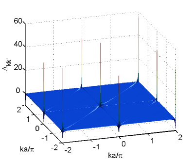
Figure 1: Noise correlations as a function of $k$ and $k^{\prime}$ for a homogeneous system with 100 hard-core bosons in 200 lattice sites.

As a function of the density $\rho=N/L$, the evolution of the noise correlations along the line $k,0$ is depicted in Fig. 2. The dips around the $k=0,\pm K$ peaks are more clearly seen in Fig. 2. As noted in Ref. Rey et al. (2006a), we find that the maximum value of $\Delta_{00}$ occurs for $\rho>0.5$, making evident the breakdown of the particle-hole symmetry for this observable.

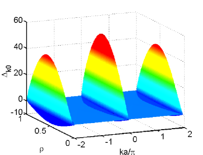
Figure 2: Noise correlations for $k^{\prime}=0$ as $k$ and $\rho$ are changed for a system with $L=200$.

In what follows, we will focus on the scaling of the $\Delta_{00}$ for different densities. For the $k=0$ peak of the momentum distribution function, it is well known that the power-law decay of the one-particle correlations results in a $n_{k=0}\sim\sqrt{L}$ scaling Lenard (1964). In Fig. 3, we show the scaling of $\Delta_{00}$ for three different densities in our periodic systems.

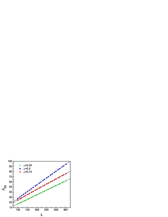
Figure 3: Scaling of the noise correlations $\Delta_{00}$ for three different densities, $\rho=$0.25, 0.5 and 0.75. The solid lines are numerical fits in the form of Eq. (24) and the results (see text) show a leading-order linear behavior.

To numerically find the scaling with system size, we assume that

$$\Delta_{00}=aL^{x}+bL^{y},$$ (24)

where $x$ and $y\ (y<x)$ describe the leading and subleading terms, respectively, and $a$ and $b$ are coefficients that, together with $x$ and $y$, are determined by means of a numerical fit. The results obtained for those four fitting parameters are given in Table 1.

Table 1: Fitting parameters for the homogeneous case.

	$\rho=0.25$	$\rho=0.5$	$\rho=0.75$
$a$	$0.17779(2)$	$0.21(9)$	$0.16(1)$
$x$	$1.00041(2)$	$1.010(3)$	$1.010(8)$
$b$	$-1.049(4)$	$0.15(7)$	$0.534(6)$
$y$	$-0.099(1)$	$0.8(1)$	$0.59(2)$

Table 1 shows that the leading term is essentially linear in all cases, while the exponent of the power law of the subleading term does depend on the density and was found to be quite close to one around half-filling. This means that in ultra-cold gas experiments one would need to reach large systems sizes to be able to clearly observe the linear scaling of the noise correlation peaks around half-filling, while this scaling would be more easily observed far away from half-filling.

IV Period-two superlattice

We now consider the case in which an additional lattice, with twice the periodicity of the original lattice, is added to the system (a superlattice). In this case, the on-site potential in Hamiltonian (1) has the form

$$V_{i}=V\cos(\pi i),$$ (25)

with $V$ representing its strength. As discussed in Ref. Rousseau et al. (2006); Rigol et al. (2006), the effect of a period-two superlattice is to open a gap of magnitude $V$ in the energy spectrum, splitting the original band into two bands. As a result, besides the usual insulating phases at $\rho=0,1$, the half-filled system in the ground state also exhibits insulating behavior. As opposed to the $\rho=0,1$ insulators, the $\rho=0.5$ (Mott) insulator does exhibit nonzero density fluctuations and a finite correlation length.

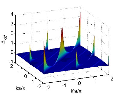
Figure 4: Noise correlations for the fractional Mott phase in the half-filled system in the presence of period-two superlattice for $L=200$.

Figure 4 shows the noise correlation pattern for the $\rho=0.5$ insulator with $V=1t$. Broad peaks can be clearly seen along the line $k=k^{\prime}$, and those are characteristic of the noise correlations in the fractional Mott phase. They contrast with the sharp peaks seen in the noise correlations of the superfluid regime studied in the previous section. The suppressed height of the peaks in Fig. 4 is a signature of the destruction of the quasi-long-range coherence in the half-filled Mott system. At this critical filling, the power-law decay of the one-particle correlations present in the absence of the superlattice is substituted by an exponential decay $\rho_{ij}\sim\exp(-|i-j|/\xi)$, for which the correlation length $\xi$ was found to be $\xi\sim 1/V$ for small values of $V$ ($V<t$) and $\xi\sim 1/\sqrt{V}$ for large values of $V$ ($V>t$) Rigol et al. (2006). As long as the lattice sizes are sufficiently large ($L\gg\xi$), the absence of quasi-long-range coherence should be clearly observed in the scaling of the noise correlations in those systems.

In the presence of the superlattice potential, additional features emerge in the noise correlations for $k=k^{\prime}\pm\pi/a$. Those can actually be used to distinguish the fractional insulator from the integer Mott insulator as both have suppressed $\Delta_{00}$ peaks but only the former has a structure in the noise correlations for $k=k^{\prime}\pm\pi/a$.

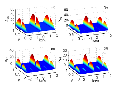
Figure 5: Noise correlations $\Delta_{k0}$ as a function of $k$ and the density for superlattice systems with (a) $V=1t$, (b) $V=2t$, (c) $V=3t$, and (d) $V=4t$. $L=200$ in all cases.

In Fig. 5, we present a unified view of the behavior of the noise correlations for different systems with a superlattice potential. There we plot $\Delta_{k0}$ as a function of $\rho$ and $k$ for four different values of $V$. Figure 5 shows that as $V$ increases from $1t$ to $4t$, the intensity of the central peak decreases for all fillings. However, the suppression is more dramatic around half-filling. The additional unique signature of the presence of a superlattice potential is the structure that can be found at $ka=\pm\pi$. It is usually a positive peak for densities below 0.5 and becomes a dip right after the density increases beyond the fractional filling insulating phase. This peak-to-dip transition was discussed in detail by Rey et al. Rey et al. (2006b, c), where in the limit $V\rightarrow\infty$ one can show analytically that $\Delta_{00}$ and $\Delta_{\pm\frac{\pi}{a}0}$ have different signs for $N=L/2+1$.

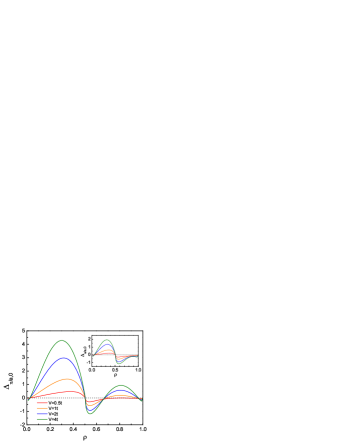
Figure 6: The sublattice peak $\Delta_{\frac{\pi}{a},0}$ as a function of $\rho$ for four different values of $V$ in systems with 200 sites. The inset shows the same quantity for systems with 100 sites.

The behavior of $\Delta_{\frac{\pi}{a}0}$ as a function of the density and for different values of $V$ can be better seen in Fig. 6. Interestingly we find that, in addition to the peak to dip transition around $\rho=0.5$, there are other dip to peak and peak to dip transitions for higher densities. Those are only apparent for sufficiently large system sizes (beyond the ones studied in Refs. Rey et al. (2006b, c)). The inset in Fig. 6 shows that for a smaller system size with only 100 sites $\Delta_{\frac{\pi}{a}0}$ is always negative for $\rho>0.5$.

Now that the generic features of the noise correlations in a superlattice potential have been reviewed, we focus on the scaling of the peaks with system size. In the fractional insulating regime, one expects that the exponential decay of correlations should lead to a saturation of the noise correlation peaks. This is, indeed, what we find, and an example is depicted in the top inset in Fig. 7 for half-filled systems with $V=t$.

In the superfluid phases, on the other hand, it has been shown that one-particle correlations decay with exactly the same power law as the homogeneous system Rigol et al. (2006). Hence, we expect to find the same leading order scaling of $\Delta_{00}$ that was discussed for homogeneous systems in the previous section. This result can be seen in the main panel of Fig. 7, and it can also be seen for the $\Delta_{\frac{\pi}{a}0}$ peak, for $\rho=0.25$, in the bottom inset.

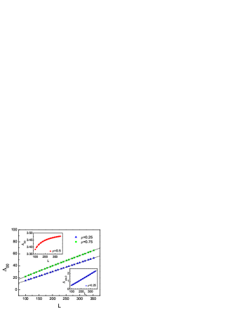
Figure 7: Scaling of $\Delta_{00}$ for $\rho=0.25$ and $\rho=0.75$ in systems with $V=1t$ and lattices with 200 sites. The top inset shows results for the same systems in the fractional ($\rho=0.5$) Mott-insulating phase. The bottom inset shows scaling of the sublattice peak $\Delta_{\frac{\pi}{a}0}$ for $\rho=0.25$ in the same systems. Solid lines are numerical fits to the results, exhibiting a leading linear scaling with $L$ in all superfluid cases.

Assuming the same scaling ansatz in Eq. (24), but in the presence of the superlattice only used for the superfluid phases, we obtain the values depicted in Table 2 for the fitting parameters

Table 2: Fitting parameters for the superlattice case.

	$k=0$		$k=\pi/a$
	$\rho=0.25$	$\rho=0.75$	$\rho=0.25$
$a$	$0.15928(6)$	$0.090(1)$	$0.00716(2)$
$x$	$0.99023(6)$	$1.045(1)$	$1.0133(3)$
$b$	$-5.2(3)$	$0.5793(5)$	$-0.03891(9)$
$y$	$-0.71(1)$	$0.636(2)$	$0.417(1)$

As expected, we find that the leading terms of the noise correlation peaks are also of order $L$ for both $\Delta_{00}$ and $\Delta_{\frac{\pi}{a}0}$. Similar to the homogeneous case, the leading linear scaling of those peaks is better seen at low densities where finite-size effects have been found to be smaller because the subleading term has a much slower scaling with system size than the leading term.

V Disordered system

The disordered case is simulated by a random on-site potential of the form

$$V_{i}=\delta\epsilon_{i},$$ (26)

where $\delta$ represents the strength of disorder and {$\epsilon_{i}$} are a set of random numbers between -1 and 1 selected with a uniform probability distribution. For our disorder calculations we usually average over between 128 and 256 disorder realizations.

For one-dimensional noninteracting fermionic systems, the presence of disorder is known to lead to Anderson localization. This is a phase in which correlations decay exponentially while the system remains compressible; that is, no gap is present in the energy spectrum. Since hard-core bosons can be mapped to noninteracting fermions, the same is known to be true for the former. We should note that despite the fact that the one-particle correlations of hard-core bosons are in general different from those of noninteracting fermions, they also decay exponentially. This is shown in Fig. 8, where we present $\rho_{x}$ (with $x=|i-j|$) for systems with different disorder strengths. One should note that the exponential decay always sets in beyond a certain distance, which decreases as the strength of the disorder increases; that is, small systems with weak disorder may behave as superfluids.

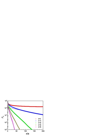
Figure 8: The decay of one-particle density matrices in half-filled systems with $L=500$, characterized by different disorder strength. The disorder averaging is performed over 128 realizations for all $\delta\neq 0$ cases. Solid lines depict exponential decay, except for the homogeneous ($\delta=0$) system, where a solid line depicts the known power law $\sqrt{x}$. Note the log-linear scale.

From the previous discussion and the results in Fig. 8 one expects that, for any given system size, the height of the noise correlation peaks should decrease with increasing disorder strength and the peaks should become broader. This can be seen in Fig. 9, where we show the noise correlations $\Delta_{kk^{\prime}}$ for four different disordered strengths in systems with 100 sites. The pattern for the $\delta=1$ case resembles that of a homogeneous superfluid system (Fig. 1), while for larger values of $\delta$ they display more similarities with the fractional Mott-insulating phase in the half-filled superlattice systems, with a clear broadening of the peaks at $k=k^{\prime}$. (Of course, no additional feature appear for $k=k^{\prime}\pm\pi/a$ in the disordered case.)

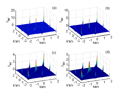
Figure 9: Disorder-averaged noise correlations as a function of $k$ and $k^{\prime}$ for systems with different disorder strength $\delta=$(a) $1t$, (b) $2t$, (c) $3t$, and (d) $4t$. $N=50$ and $L=100$ for all cases and the average was performed over 128 disorder realizations.

A comparison between the cross-sectional view (for $k^{\prime}=0$) of the noise correlations in all three phases discussed previously, namely, the superfluid, fractional Mott, and glassy phases, is shown in Fig. 10. This comparison makes evident (i) the suppression of the $\Delta_{00}$ peak in the fractional Mott and glassy phases, (ii) the fact that the two insulating phases can be distinguished by the superlattice-induced features at $k=k^{\prime}\pm\pi$, and (iii) that the disordered Anderson-glass and the superfluid phase exhibit the same satellite dips accompanying the $\Delta_{00}$ peaks, while the dips vanish rather quickly in the fractional Mott phase.

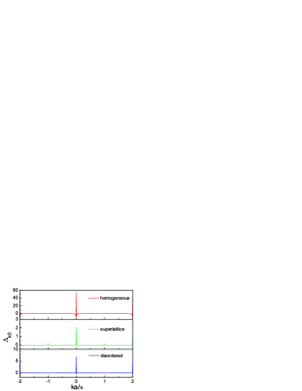
Figure 10: Noise correlations with fixed $k^{\prime}=0$ for three half-filled systems with $L=200$. The superfluid phase, the fractional Mott phase, and the Anderson-glass phase are associated with the homogeneous, period-two superlattice ($V=2t$), and disordered ($\delta=2t$) cases, respectively. The average is performed over 256 disorder realizations.

Similar to the behavior of the fractional Mott phase, one also expects that as the system size increases for any nonzero value of the disorder strength, the $\Delta_{00}$ will saturate to a size-independent value that will only be a function of the density and the disorder strength. This behavior is shown in Fig. 11 for three different values of the disorder strength and for systems with up to 200 sites.

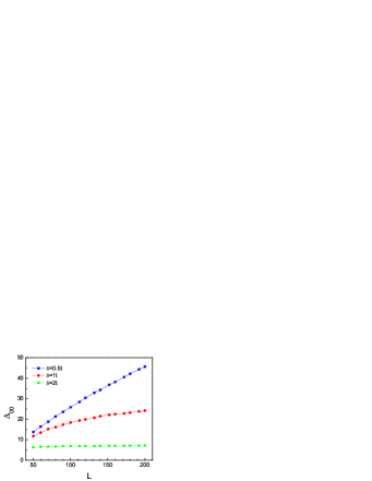
Figure 11: Scaling of the noise correlations $\Delta_{00}$ for three different values of $\delta$ in half-filled systems.

Finally, we study how the $\Delta_{00}$ peak in the noise correlations behaves as a function of the disorder strength for a fixed size of the lattice. Since for $\delta=0$ we have already shown that such a peak diverges with system size, in the following we analyze how $\Delta_{00}$ decreases as the disorder strength increases.

In Fig. 12, we show $\Delta_{00}$ as a function of $\delta$ for two different system sizes. Three different regimes can be clearly identified. (i) For small values of $\delta$, $\Delta_{00}$ approximately stays constant with the increase of $\delta$, which can be understood to be a consequence of a correlation length that exceeds the system size. As seen in Fig.12, that region decreases as the system size increases. (ii) As $\delta$ increases even further, a power-law decay develops in $\Delta_{00}$, and the region over which such a power law can be seen increases with system size as regime (i) is suppressed. In our fits, we find the power law $\Delta_{00}\sim\delta^{-\gamma}$ to have an exponent $\gamma\sim 1.78(2)$, but it is still influenced by some finite-size effects. In order to gain further understanding of the power-law decay of the height of this noise peak in insulating phases, we have studied the behavior of $\Delta_{00}$ vs $V$ in the fractional Mott phase in a superlattice, for which we can study larger systems sizes. We find that $\Delta_{00}\sim V^{-\gamma}$ with an exponent of $0.874(5)$, which is different from the one for the disordered system. These results clearly show that the power-law decay of $\Delta_{00}$ as one enters an insulating phase depends on the perturbation creating the insulator, i.e., it is not universal. (iii) Finally, for very strong disorder, $\Delta_{00}$ saturates to a nonzero value. This asymptotic behavior is found to agree with the analytical value in the $\delta\rightarrow\infty$ limit, computed using

$$\Delta_{00}=\rho(\rho+1),$$ (27)

which was derived by Rey et al. Rey et al. (2006b). Equation (27) shows that $\Delta_{00}$ only depends on the density and also makes explicit the absence of particle-hole symmetry for this observable in hard-core-boson systems. This third regime is robust against the disorder variance, something that follows from the fact that the correlation length is of the order of or smaller than the lattice spacing $a$.

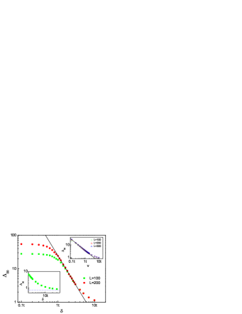
Figure 12: Noise correlation peaks $\Delta_{00}$ as a function of disorder strength in two half-filled disordered systems with $L=$100 and 200, respectively. The solid line shows a power-law fit $\Delta_{00}\sim\delta^{-\gamma}$, with $\gamma=1.78(2)$ in the range from $\delta=t$ to $3t$ for $L=200$. The top inset shows $\Delta_{00}$ as a function of $V$ in three half-filled period-two superlattices. The solid line depicts a power law with an exponent $\gamma=0.874(5)$. The bottom inset shows the asymptotic behavior for large values of $\delta$; the dotted line marks the analytical result in the limit of infinite disorder.

VI Conclusions

We have implemented an exact approach to numerically compute the noise correlations for hard-core boson in one-dimensional lattices. For that purpose, we have extended to four-point correlations the recipe for calculating two-point correlations introduced in Refs. Rigol and Muramatsu (2004, 2005). Our approach has a polynomial time scaling that is more efficient than the straightforward application of Wicks theorem, and can be easily extended to study noise correlations in nonequilibrium systems.

We have applied this approach to study the scaling of noise correlations in three different phases that appear in homogeneous systems and in the presence of two different background potentials. We have shown that in the superfluid phase, the noise correlation peaks $\Delta_{00}$ exhibit a leading linear behavior $\sim L$, independent of the density and of the presence of a superlattice potential. The subleading term was found to be strongly dependent on the latter two. On the other hand, the fractional Mott and Anderson-glass insulating phases exhibit an asymptotic value, which is independent of system size and only depends on the density and the strength of the potentials creating such phases. This behavior was expected and manifests the absence of quasi-long-range order in these two phases.

In the period-two superlattice, we have also found various peak-to-dip and dip-to-peak transitions that were not observed in previous studies with smaller system sizes, something that demonstrates the importance of finite-size effects in the noise correlations and the need for approaches that allow one to study very large system sizes.

Finally, we have shown that in the disordered system (fractional Mott phase), the decrease of the $\Delta_{00}$ peak with increasing disorder strength (superlattice strength) exhibits a region with a power-law decay $\Delta_{00}\sim\delta(V)^{-\gamma}$, with a nonuniversal value of exponent $\gamma$ that depends on the kind of perturbation creating the insulator.