Dependence of the Macroscopic Quantum Tunneling Rate on Josephson Junction Area

Abstract

We have carried out systematic Macroscopic Quantum Tunneling (MQT) experiments on Nb/Al-AlO_x/Nb Josephson junctions (JJs) of different areas. Employing on-chip lumped element inductors, we have decoupled the JJs from their environmental line impedances at the frequencies relevant for MQT. This allowed us to study the crossover from the thermal to the quantum regime in the low damping limit. A clear reduction of the crossover temperature with increasing JJ size is observed and found to be in excellent agreement with theory. All junctions were realized on the same chip and were thoroughly characterized before the quantum measurements.

I Introduction

Since the gauge-invariant phase over a Josephson junction (JJ) $\varphi$ is a macroscopic variable, circuits containing JJs have been used as model systems for the investigation of quantum dynamics on a macroscopic scale. This research has recently led to the development of different types of superconducting quantum bits Nakamura et al. (1999); Friedman et al. (2000); Martinis et al. (2002); Vion et al. (2002); Chiorescu et al. (2003), which are promising candidates for the implementation of quantum computers. The starting point of this field was the observation of Macroscopic Quantum Tunneling (MQT) in Josephson junctions in the 1980s Voss and Webb (1981); Martinis et al. (1987). In such experiments, the macroscopic variable $\varphi$ is trapped in the local minimum of a tilted washboard potential, before it tunnels through the potential barrier and starts rolling down the sloped potential. Since this running state is equivalent to the occurrence of a voltage drop over the junction, such tunneling events can be experimentally detected. MQT—often referred to as secondary quantum effect—is the manifestation of the quantum mechanical behavior of a single macroscopic degree of freedom in a complex quantum system. Furthermore, it is the main effect on which all quantum devices operated in the phase regime (such as phase qubits and flux qubits) are based. Consequently, the detailed understanding of MQT is not only interesting by itself, but also important for current research on superconducting qubits operated in the phase regime. In this article, we report on a systematic experimental study of the dependence of the macroscopic quantum tunneling rate on the Josephson junction area, which to our knowledge has never been performed before. As usualVoss and Webb (1981); Martinis et al. (1987); Wallraff et al. (2003), we measure the rate at which the escape of $\varphi$ out of the local minimum of the washboard potential occurs as a function of temperature. At high temperatures, the escape is driven by thermal fluctuation over the barrier while it is dominated by tunneling at low temperatures. This leads to a characteristic saturation of the temperature dependent tunneling rate below a crossover temperature $T_{\mathrm{cr}}$, which is the hallmark of MQT. The rates above and below crossover are affected by the dissipative coupling to the environment of the JJ, which is commonly accounted for by a quality factor $Q$ in theoretical descriptions. A major goal of the presented study was to keep the influence of $Q$ on the rate constant while varying the junction area, so that a change in the observed escape rates could be clearly assigned to the changed JJ size. For this purpose, we work in the underdamped regime of large $Q$, which is only possible if the JJ is to some extent decoupled from its low-impedance environment (i.e. the transmission line leading to the JJ). We achieve this by employing on-chip lumped element inductors.

This article is organized as follows: First, the physical model of MQT is discussed and the theoretical expectations for varying junction size are given. Second, the procedure and setup of measurement are described. Afterwards, the investigated Josephson junctions are characterized carefully, and finally, the results of the MQT measurements are presented and discussed.

II Model and Macroscopic Quantum Tunneling

II.1 General Model

The dynamics of a JJ is usually described by the RCSJ (resistively and capacitively shunted junction) model Stewart (1968); McCumber (1968). The current flowing into the connecting leads comprises in addition to the Josephson current $I_{J}=I_{c}\sin\varphi$ ($I_{c}$ denotes the critical current of the junction) a displacement current due to a shunting capacitance $C$ and a dissipative component due to a frequency dependent shunting resistance $R$. For a complete description, the electromagnetic environment given by the measurement setup can be included in the model parameters. In our case, $R$ will be influenced by the environmental impedance while $C$ can be regarded as solely determined by the plate capacitor geometry of the JJ itself. In any case, the bias current $I$ is composed of

$$I=I_{c}\sin\varphi+\frac{1}{R}\frac{\Phi_{0}}{2\pi}\dot{\varphi}+C\frac{\Phi_{0}}{2\pi}\ddot{\varphi}\,,$$ (1)

where $\varphi$ is the gauge-invariant phase difference across the junction and $\Phi_{0}=h/2e$ is the magnetic flux quantum. The dynamics of $\varphi$ as expressed by (1) is equally described by the well-studied Langevin equation

$$M\ddot{\varphi}+\eta{}M\dot{\varphi}+\frac{\partial{}U}{\partial{}\varphi}=\xi(t)\,,$$ (2)

which describes a particle of mass $M=C(\Phi_{0}/2\pi)^{2}$ in a tilted washboard potential

$$U\left(\varphi\right)=E_{J}\left(1-\cos\varphi-\gamma\varphi\right)\,,$$ (3)

exposed to damping $\eta=1/RC$ and under the influence of a fluctuating force $\xi(t)$. The strength of $\xi(t)$ is linked to temperature and damping by the fluctuation-dissipation theorem. Furthermore, $\gamma=I/I_{c}$ denotes the normalized bias current while $E_{J}=\Phi_{0}I_{c}/2\pi$ is called the Josephson coupling energy. For $\gamma<1$, if thermal and quantum fluctuations are ignored, the particle is trapped behind a potential barrier

$$\Delta U=2E_{J}\left(\sqrt{1-\gamma^{2}}-\gamma\arccos\gamma\right)\,,$$ (4)

and the JJ stays in the zero-voltage state. In the potential well, the phase oscillates with the bias current dependent plasma frequency

$$\omega_{p}=\omega_{p0}\left(1-\gamma^{2}\right)^{1/4}=\sqrt{\frac{2\pi I_{c}}{\Phi_{0}C}}\left(1-\gamma^{2}\right)^{1/4}\,.$$ (5)

To complete the list of important system parameters given in this section, we introduce the quality factor

$$Q=\omega_{p}/\eta=\omega_{p}RC\,,$$ (6)

which is conventionally used to quantify the damping in the JJ.

At finite temperatures, the thermal energy $k_{B}T$ ($k_{B}$ being Boltzmann’s constant) described by $\xi(t)$ in (2) can lift the phase particle over the potential barrier before the critical current $\gamma=1$ is reached, so that the particle will start rolling down the potential. This is called premature switching and the observed maximal supercurrent $I_{\mathrm{sw}}<I_{c}$ is called the switching current. When the phase particle is rolling, the JJ is in the voltage state, since a voltage drop according to $\dot{\varphi}=(2\pi/\Phi_{0})V$ is observed. The thermal escape from the potential well occurs with a rate Kramers (1940); Hänggi et al. (1990)

$$\Gamma_{\mathrm{th}}=a_{t}\frac{\omega_{p}}{2\pi}\exp\left(-\frac{\Delta U}{k_{B}T}\right)\,,$$ (7)

where $a_{t}$ is a temperature and damping dependent prefactor, which will be discussed in more detail in Sec. II.3.

For $T\rightarrow 0$, where $\Gamma_{\mathrm{th}}\rightarrow 0$, premature switching will still be present due to quantum tunneling through the potential barrier. As the phase difference over the JJ is a macroscopic variable, this phenomenon is often referred to as ”Macroscopic Quantum Tunneling” (MQT). This means that by measuring the switching events of a JJ for decreasing temperature, one will see a temperature dependent behavior (dominated by the Arrhenius factor $\exp(-\Delta{}U/k_{B}T)$ in (7)) until a crossover to the quantum regime is observed. The crossover temperature $T_{\mathrm{cr}}$ is approximately given by Affleck (1981); Martinis et al. (1987)

$$T_{\mathrm{cr}}=\frac{\hbar\omega_{p}}{2\pi k_{B}}=\frac{\hbar\omega_{p0}}{2\pi{}k_{B}}\cdot(1-\gamma^{2})^{1/4}\,,$$ (8)

where $\hbar$ is Planck’s constant. We can write the quantum tunneling rate for temperatures well below crossover as Caldeira and Leggett (1983); Martinis et al. (1987); Grabert et al. (1987); Freidkin et al. (1988)

$$\Gamma_{q}=a_{q}\frac{\omega_{p}}{2\pi}\exp(-B)\,,$$ (9)

where $a_{q}=\sqrt{864\pi\Delta{}U/\hbar{}\omega_{p}}\exp(1.430/Q)$ and $B=(36\Delta U/5\hbar\omega_{p})(1+0.87/Q).$ In the limit of large $Q$, the escape rate is expected to approach the temperature independent expression (9) quicklyGrabert et al. (1987); Freidkin et al. (1986); *Freidkin87 once the temperature falls below $T_{\mathrm{cr}}.$ The rates in (7) and (9) are functions of the normalized bias current $\gamma$ via (4) and (5). The crossover to the quantum regime can be nicely visualized by measuring the bias current dependence of the escape rate $\Gamma(I)$ for a sequence of falling temperatures. The data are then described over the whole temperature range by the thermal rate (7) with the temperature as a fitting parameter. In this way, one obtains a virtual ”escape temperature” $T_{\mathrm{esc}}$, which can be compared to the actual bath temperature $T$. In the thermal regime, one should obtain $T_{\mathrm{esc}}=T$ while in the quantum regime, one should get $T_{\mathrm{esc}}=T_{\mathrm{cr}}=\mathrm{const}$.

II.2 Influence of JJ Size on MQT

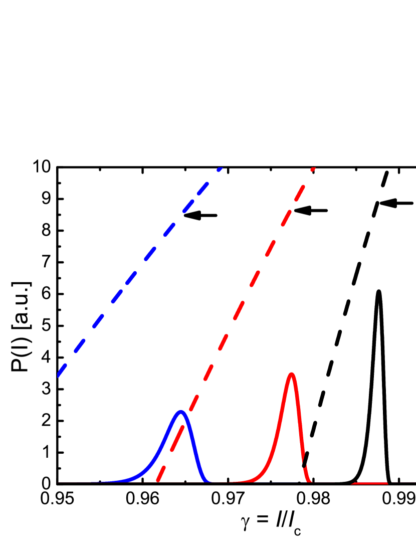
Figure 1: Theoretically calculated switching current distributions $P(I)$ (solid curves) and quantum tunneling rates $\Gamma_{q}$ (dashed curves) for samples B1 (left) to B3 (right) having different diameters $d$ (for parameters see Tab. 1). The difference in $\gamma_{\mathrm{cr}}$ (maximum position of $P(I)$), where quantum tunneling leads to escape from the potential well, is significant. The tunneling rates at these points (marked by arrows) are of the order of $\approx 100$ kHz for all samples.

The crucial element of a Nb-based Josephson junction as employed in this work is the Nb/Al-AlO_x/Nb trilayer. For a JJ, $I_{c}=j_{c}\cdot A$ and $C=c\cdot A$, where the critical current density $j_{c}$ and the specific capacitance $c$ are constant for a given trilayer and $A$ is the area of the junction. Hence, by reformulating (5), we find that $\omega_{p0}=\sqrt{2\pi j_{c}/\Phi_{0}c}$, meaning that for JJs fabricated with the same trilayer, the plasma frequency does not depend on their size. So at first sight, the crossover temperature (8) should also be independent of the JJ size. In reality, however, the problem is more subtle, as one needs to take into account at which normalized bias current $\gamma_{\mathrm{cr}}$ the quantum tunneling rate (9) becomes significant. Since the height of the potential barrier $\Delta U\propto E_{J}\propto A$ is proportional to the JJ size, a significant tunneling rate should be reached at different $\gamma_{\mathrm{cr}}$ values for junctions of different size. These points can be estimated by theoretically calculating (9) and converting it into a switching current histogram, as it would be observed in a real experiment. The probability distributions of switching currents $P(\gamma)$ can be obtained from the quantum rate by equating Fulton and Dunkleberger (1974)

$$P(\gamma)=\Gamma_{q}\left(\frac{{\rm d}\gamma}{{\rm d}t}\right)^{-1}\left(1-\int_{0}^{I}P(u){\rm d}u\right)\,,$$ (10)

where ${\rm d}\gamma/{\rm d}t=(1/I_{c})\cdot({\rm d}I/{\rm d}t)$ is a constant for the linear current ramp chosen in our experiment. For the parameters of the junctions investigated in this work (see Tab. 1), the switching current distributions $P(\gamma)$ were determined with a quality factor of $Q=100$ and a current ramp rate of 100 Hz, according to our experiments (see below). They are shown in Fig. 1, where it can be seen that the $\gamma_{\mathrm{cr}}$ values (the positions of the maxima of the distributions) significantly and systematically increase with the junction size. Evaluation of the $\Gamma_{q}(\gamma_{\mathrm{cr}})$ values for the samples indicates that quantum tunneling will be experimentally observable at a rate of around $\Gamma_{q}\approx 10^{5}$ Hz.

Subsequently, the expected crossover temperature was calculated from (8) with $\gamma=\gamma_{\mathrm{cr}}$. The sample parameters as well as the expected $\gamma_{\mathrm{cr}}$ and $T_{\mathrm{cr}}$ values are given in Table 1. It can be seen that due to the term in parenthesis on the right hand side of (8), the crossover temperature systematically decreases for increasing junction size. The change in $T_{\mathrm{cr}}$ is large enough to be observed experimentally. However, such a systematic study of the size-dependence of $T_{\mathrm{cr}}$ has never been carried out before.

Table 1: Parameters of the investigated samples and calculated $\gamma_{\mathrm{cr}}$ and $T_{\mathrm{cr}}$ values. The critical current density accounts for $j_{\mathrm{c}}\approx 650$ A/cm² while the specific capacitance of $c=55$ fF/µm² was recently determined by the measurement of Fiske steps on a trilayer prepared in our lab under identical conditions. Parasitic capacitances due to idle regions next to the JJs have been taken into account for all calculations in this article. For the calculation of $T_{\mathrm{cr}}$, the actual measured critical currents were used.

Sample	Diameter $d$ (µm)	$\gamma_{\mathrm{cr}}$	$T_{\mathrm{cr}}$ (mK)
B1	$1.9$	$0.965$	$371$
B2	$2.55$	$0.977$	$323$
B3	$3.6$	$0.988$	$291$
B4	$3.8$	$0.988$	$277$

II.3 Influence of Damping on MQT

The quality parameter $Q$ is frequently employed to describe the strength of the hysteresis in the current-voltage characteristics of a JJ. In this case, one often takes $Q=\omega_{p0}R_{\mathrm{sg}}C$ with $R_{\mathrm{sg}}$ being the subgap resistance of the junction. Here, $Q$ is size-independent, as $R_{\mathrm{sg}}\propto 1/A$ and $C\propto A$. In the context of MQT, however, the dynamics takes place at a frequency of $\omega_{p}$, so that a complex impedance at that frequency $Z(\omega_{p})$ has to be considered. For an MQT experiment, where the phase and not the charge is the well-defined quantum variable, the admittance $Y(\omega_{p})$ will be responsible for damping G. L. Ingold and Yu. V. Nazarov: Charge Tunneling Rates in Ultrasmall Junctions (1992), so that $R$ in (6) will be given by $R=1/{\rm Re}{(Y)}$.

If the junction was an isolated system, the value of $R$ in the context of MQT would be determined by the intrinsic damping in the zero-voltage state. The value which is typically taken as a measure for this is the maximal subgap resistance $R_{\mathrm{sg,max}}$, which is simply the maximal resistance value which can be extracted from the nonlinear subgap branch of the current-voltage characteristics Milliken et al. (2004); Gubrud et al. (2001). In most experiments however, the electromagnetic environment of the JJ can be assumed to have an impedance that is real and accounts for $Z_{0}\approx 100$ $\Omega$, corresponding to typical transmission lines Martinis et al. (1987). As furthermore $Z_{0}\ll R_{\mathrm{sg,max}}$ and both contributions are in parallel (see Fig. 2a), we can simply write $Q=\omega_{p}Z_{0}C$ in this case.

Evidently, for junctions having a small capacitance (as in our experiment), the quality factor $Q=\omega_{p}Z_{0}C$ will be limited to $Q\lesssim 10$ and additionally depend on the JJ size like $C\propto A$. As we want to investigate the pure influence of the JJ size on MQT, we would like to obtain very low damping as well as similar damping for all investigated junctions. In the implementation of phase qubits, current biased Josephson junctions have been inductively decoupled from their environment by the use of circuits containing lumped element inductors and an additional filter junction Martinis et al. (2002). In order to keep our circuits simple, we attempted to reach a similar decoupling by only using on-chip lumped element inductors right in front of the JJs (see Fig. 2b). This setup leads to an admittance

$$Y=1/R_{\mathrm{sg,max}}+1/(Z_{0}+i\omega L)\,.$$ (11)

As for (11), we find ${\rm Re}{(Y)}\rightarrow 1/R_{\mathrm{sg,max}}$ in the limit $\omega L\rightarrow\infty$, big enough lumped element inductances should decouple the JJ from the $Z_{0}$ environment and result in a high intrinsic quality factor $Q=\omega_{p}R_{\mathrm{sg,max}}C$ even for switching experiments. Although it might be difficult to reach this limit in a real experiment, decoupling inductors should definitively help to increase the quality factor and move towards a JJ-size independent damping.

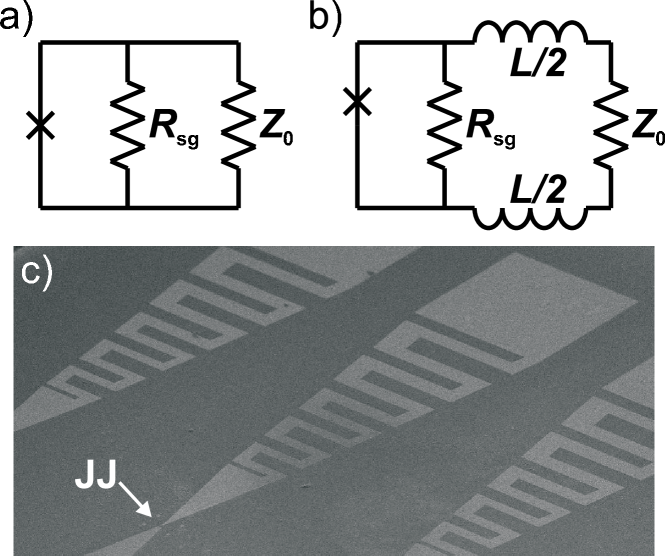
Figure 2: a) Typical impedance environment for switching experiments in a JJ. As $Z_{0}\ll R_{\mathrm{sg}}$, the junction sees the impedance $Z_{0}$ at the plasma frequency. b) Lumped element inductors $L$ can be used to decouple the JJ from the line impedance $Z_{0}$, as discussed in the text. c) SEM micrograph of the electrode design used for the investigated junctions.

The damping in the JJ influences the thermal escape rate (7) via the prefactor $a_{t}<1$, which has been calculated for the first time by Kramers in 1940Kramers (1940). In the limiting case $Q\rightarrow 0$ (moderate to high damping), he found:

$$a_{t}=\alpha_{\mathrm{KMD}}=\sqrt{1+\left(\frac{1}{2Q}\right)^{2}}-\frac{1}{2Q}\,,$$

while in the opposite limit $Q\rightarrow\infty$ (very low damping limit), he found:

$$a_{t}=\alpha_{\mathrm{KLD}}=\frac{36\Delta{}U}{5Qk_{B}T}\,.$$

More recently, Büttiker, Harris and LandauerBüttiker et al. (1983) extended the very low damping limit to the regime of low to moderate damping finding the expression

$$a_{t}=\frac{4}{(\sqrt{1+4/\alpha_{\mathrm{KLD}}}+1)^{2}}\,.$$ (12)

Additionally, damping reduces the crossover temperature according to Grabert and Weiss (1984); Hänggi et al. (1990)

$$T_{\mathrm{cr,Q}}=\frac{\hbar\omega_{p}}{2\pi k_{B}}\cdot\alpha_{\mathrm{KMD}}\,.$$ (13)

A possible way to determine the quality factor $Q$ for such quantum measurements is to extract it from spectroscopy data Martinis et al. (1987). Unfortunately, for samples with such a high critical current density as used in our experiments described here, this turns out to be experimentally very hard. Hence, we will limit the analysis of the damping in our experiments to the MQT measurements. However, other groups have found a good agreement between the $Q$ values determined by spectroscopy and by MQT Martinis et al. (1987); Wallraff et al. (2003) and we hope to observe such a major increase in $Q$ due to the decoupling inductors that minor uncertainties in $Q$ should not play a role.

III Setup and Procedure of Measurement

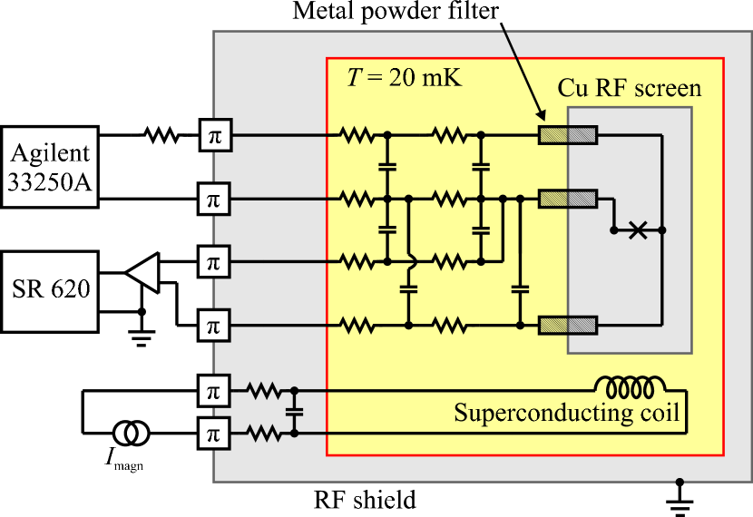
Figure 3: Schematic overview of the measurement system. The superconducting coil and the sample are inside a magnetic shield consisting of three nested cylindrical beakers, the middle one made from Pb, the two remaining ones from Cryoperm. Furthermore, the entire dilution refrigerator is placed inside a $\mu$-metal shield at room temperature. The $\pi$-symbols denote commercial $\pi$-filters.

All samples were fabricated by a combined photolithography / electron beam lithography process based on Nb/Al-AlO_x/Nb trilayers. The trilayer deposition was optimized carefully in order to obtain stress-free Nb films. For the definition of the Josephson junctions, an Al hard mask is created employing electron beam lithography. This hard mask acts as an ideal etch stopper during the JJ patterning with reactive-ion-etching. Furthermore, it allows the usage of anodic oxidation even for small junctions, which would not be possible if a resist mask was used. After the anodic oxidation, the Al hard mask is removed by a wet etching process. Details of this Al hard mask technique and the entire fabrication process are discussed elsewhere Kai (2010).

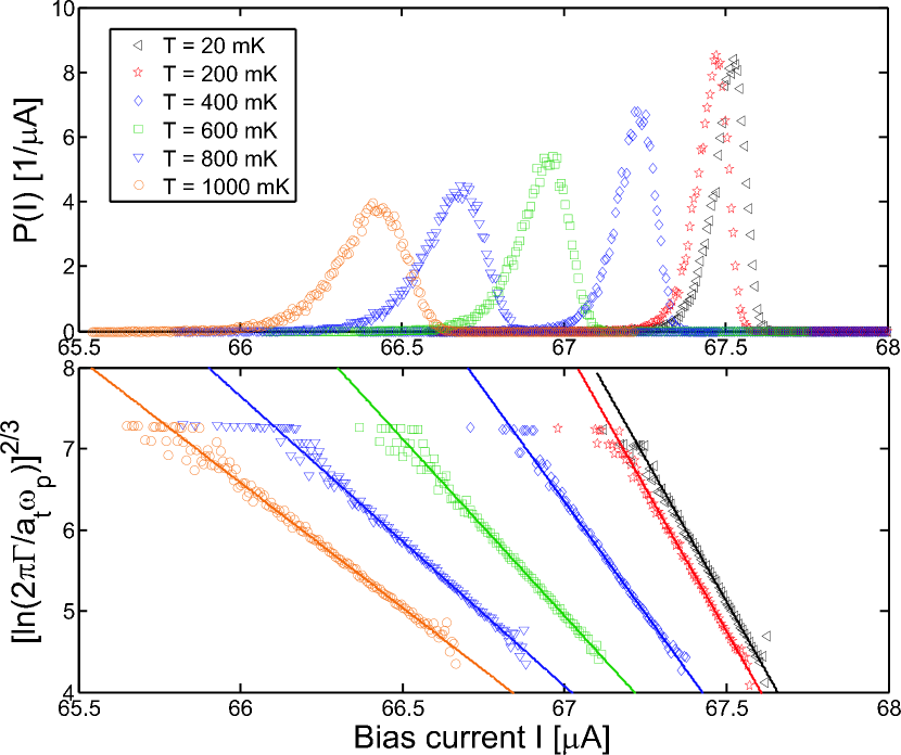
Figure 4: Top: The measured switching current histograms for sample B3 for selected temperatures. For increasing $T$, the switching currents decrease and the histograms broaden. Bottom: The plot obtained by applying (15) for the same sample. The fits allow to extract $T_{\mathrm{esc}}$ as well as $I_{c}$.

Our measurement setup can be seen in Fig. 3. Special care has been taken in design of the filtering stages in order to reach a low-noise measurement environment. The goal of the measurement is to determine the escape rate $\Gamma$. In order to do so, we have measured the probability distribution $P(I)$ of switching currents. This was done by ramping up the bias current with a constant rate $\dot{I}={\rm d}I/{\rm d}t$ and measuring the time $t_{\mathrm{sw}}$ between $I=0$ and the switching to the voltage state with a Stanford Research 620 Counter, so that $I_{\mathrm{sw}}=\dot{I}\cdot t_{\mathrm{sw}}$ could be calculated. An Agilent 33250A waveform generator was used to create a sawtooth voltage signal with a frequency of 100 Hz, which was converted into the bias current by a resistor of $47\,{\rm k}\Omega$. In this way, for each temperature, $I_{\mathrm{sw}}$ could be measured repeatedly. After doing so 20,000 times, the switching current histograms $P(I)$ with a certain channel width $\Delta I$ were attained as shown in the upper part of Fig. 4. These histograms were then used to reconstruct the escape rate out of the potential well as a function of the bias current by employing Martinis et al. (1987); Fulton and Dunkleberger (1974)

$$\Gamma(I)=\frac{\dot{I}}{\Delta I}\ln\frac{\sum_{i\geq I}{P(i)}}{\sum_{i\geq I+\Delta I}{P(i)}}\,.$$ (14)

With $\Gamma$ at hand, we could now determine the escape temperature $T_{\mathrm{esc}}$ by employing (7). In order to be able to rearrange this formula, we approximate the potential barrier in the limit $\gamma\rightarrow 1$ as $\Delta U=4\sqrt{2}/3\cdot E_{J}\cdot(1-\gamma)^{3/2}$, so that we find

$$\left(\ln\frac{2\pi\Gamma(I)}{a_{t}(I)\omega_{p}(I)}\right)^{2/3}=\left(\frac{4\sqrt{2}E_{J}}{3k_{B}T_{\mathrm{esc}}}\right)^{2/3}\frac{I_{c}-I}{I_{c}}\,.$$ (15)

Hence, by plotting the left side of (15) over the bias current $I$, we should obtain straight lines (see bottom part of Fig. 4). Consequently, we can extract the theoretical critical current $I_{c}$ in the absence of any fluctuations as well as the escape temperature $T_{\mathrm{esc}}$ by applying a linear fit with slope $a$ and offset $b$. We then find

$$I_{c}=-\frac{b}{a}\qquad\mathrm{and}\qquad T_{\mathrm{esc}}=-\frac{4\sqrt{2}\Phi_{0}}{6\pi k_{B}a\sqrt{b}}\,.$$

Since $I_{c}$ enters (15) via $E_{J}$ and $\omega_{p}$, this fitting procedure has to be iteratively repeated until the value of $I_{c}$ converges. So strictly speaking, this procedure involves two fitting parameters, namely $T_{\mathrm{esc}}$ and $I_{c}$. However, it turns out that $I_{c}$ is temperature independent within the expected experimental uncertainty (for all our measurements, the fit values of $I_{c}$ vary over the entire temperature range with a standard deviation of only around 0.09 %). Furthermore, the found $I_{c}$ values agree very well with the expected ones from the critical current density $j_{c}$ of the trilayer and the junction geometry. Altogether, it can be said that the results for the main fitting parameter $T_{\mathrm{esc}}$ should be very reliable.

IV Sample Characterization

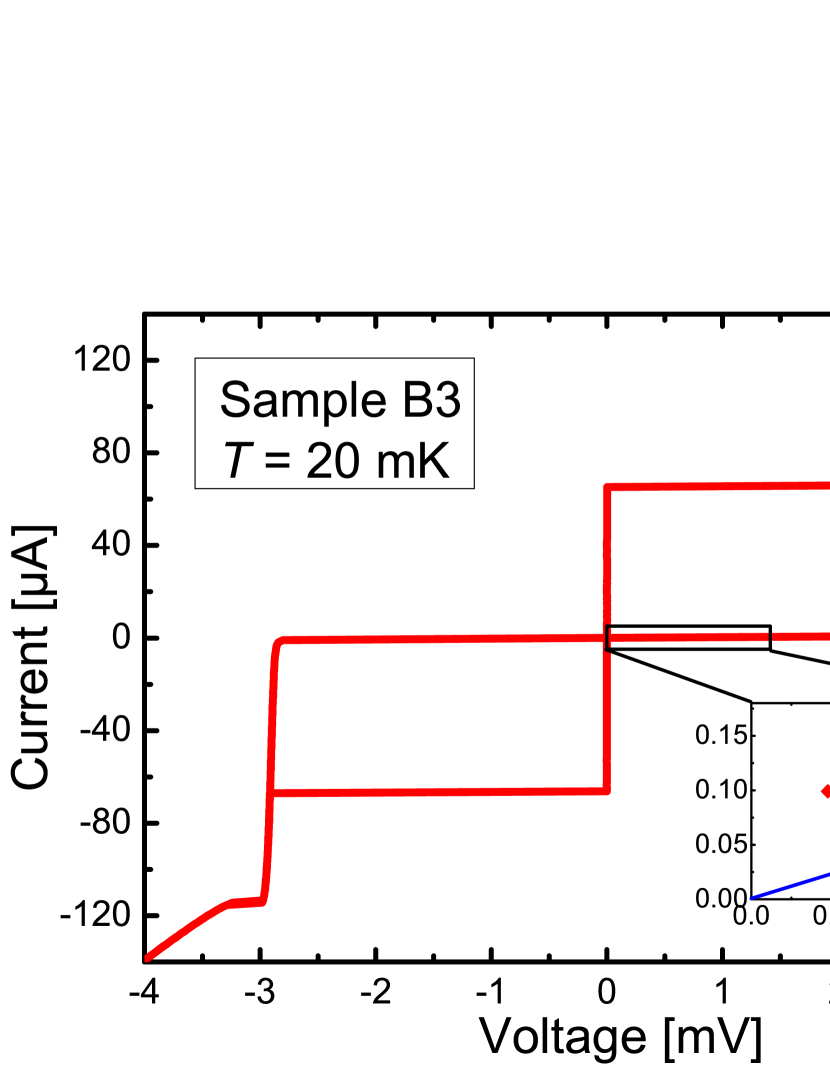
Figure 5: Characterization of sample B3. The $IV$ curve shows the high quality regarding the $I_{c}R_{N}$ ratio as well as low subgap currents. The inset shows a magnification of the subgap branch achieved by a voltage bias. The blue line illustrates how the value for $R_{\mathrm{sg,max}}$ was determined. The fact that the current rises for decreasing voltage at $V\approx 0.5$ V is due to the fact that the junction jumps back to a supercurrent $I\neq 0$ for $V=0$.

The JJs were circular in shape and their geometries are given in Table 1. In order to characterize the samples, $IV$ curves with current bias as well as $IV$ curves with voltage bias were recorded (an example can be seen in Fig. 5). The quality parameters for all samples are given in Table 2 and indicate a very high quality. In the voltage bias measurements, two major current drops at voltages $2\Delta/2$ and $2\Delta/3$ could be seen and attributed to Andreev reflections Arnold (1987). Below $2\Delta/3$, we were able to extract values of the maximal subgap resistance $R_{\mathrm{sg,max}}$ as illustrated by the blue line in Fig. 5.

Table 2: Experimentally determined parameters for all investigated JJs. The theoretical critical currents $I_{c}$ were extracted from the MQT measurements. The $R_{\mathrm{sg,max}}$ values were obtained as shown in the inset of Fig. 5a.

Sample	$I_{c}$ (µA)	$V_{\mathrm{gap}}$ (mV)	$I_{c}R_{N}$ (mV)	$R_{\mathrm{sg,max}}$ (k$\Omega$)
B-1	$19.1$	2.88	$1.75$	$54.0$
B-2	$31.9$	2.88	$1.86$	$73.0$
B-3	$68.1$	2.92	$1.93$	$21.1$
B-4	$70.8$	2.90	$1.91$	$31.5$

V Results and Discussion

V.1 Damping in the Junctions

In order to decouple the JJs from their environmental impedance, the electrodes leading to the junctions were realized as lumped element inductors, as can be seen in Fig. 2c. This design was based on the layout that we recently used to successfully realize lumped element inductors for $LC$ circuits in the GHz frequency range Kaiser et al. (2010). Furthermore, simulations with Sonnet confirmed that the meandered electrodes indeed act as lumped element inductors at the relevant frequencies $\omega_{p}(\gamma_{\mathrm{cr}})$. The complex simulation with Sonnet gives an inductance of $L/2\approx 1.65\,$nH (for one electrode) while the much simpler analysis with FastHenry yields $L/2\approx 1.8\,$nH.

For each sample, the data were analyzed using a number of different $Q$ values in order to see if we could determine the experimentally observed damping. This was done by calculating the deviation of $T_{\mathrm{esc}}$ from the bath temperature $T$ in the thermal regime:

$$\Delta T^{2}=\sum_{T>500\,{\rm mK}}\left(T_{\mathrm{esc}}-T\right)^{2}$$ (16)

and finding its minimum value regarding $Q$. The corresponding values were then used for the sample analysis. It can be seen in Fig. 6 that the points of experimentally observed damping could be clearly identified. The evaluated $Q$ values are given in Table 3.

In a preliminary experiment, we investigated MQT in a junction with a diameter of $d=1.9$ µm, a critical current of $I_{c}\approx 12$ µA and low-inductance electrodes, which were simple wide lines and can be imagined as the envelope of the electrodes in Fig. 2c. We carried out a similar analysis to determine the damping and obtained a quality factor of $Q=4$. Subsequently, we evaluated (6) and calculated an impedance of $R=99.8$ $\Omega$, which is very close to the expected value of $Z_{0}\approx 100$ $\Omega$ for typical transmission lines Martinis et al. (1987). This means that with this simple preliminary design, the junction was in no way decoupled from the electromagnetic environment.

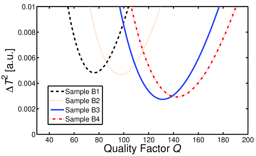
Figure 6: Determination of the experimentally observed quality factor $Q$ for all samples. The curves are minimal when the determined $T_{\mathrm{esc}}$ values deviate the least from the corresponding bath temperatures $T$ in the thermal regime $T>500$ mK.

The $Q$ values obtained by using inductive electrodes (see Tab. 3), however, show that we have drastically increased the quality factors with respect to the preliminary measurement. If we calculate the $R$ values using (6), we find that they are clearly above the typical line impedance of $Z_{0}\approx 100$ $\Omega$ as well as the vacuum impedance of 377 $\Omega$, which shows that we were indeed able to inductively decouple the JJ from its usual impedance environment. As expected, the determined $R$ values are still clearly below the subgap resistance $R_{\mathrm{sg,max}}$, indicating that we have not reached the limit $\omega L\rightarrow\infty$. Instead, we are in the intermediate regime $Z_{0}\ll R\ll R_{\mathrm{sg,max}}$, leading to the fact that $Q$ still exhibits a slight dependence on the JJ size (see Table 3). However, all JJs are in the low-damping regime, so that no influence of damping on the results should be present and differences in the experimental results should indeed be due to the JJ size. This can be seen by the fact that the damping related correction in $T_{\mathrm{cr}}$ according to equation (13) is smaller than 1 % for all experimentally observed $Q$ values. Altogether, we can state that we will be able to carry out our investigation of the size dependence of MQT with very low and nearly size-independent damping.

Table 3: The experimentally determined values characterizing the damping for all samples. The $L_{\mathrm{calc}}$ values were determined from $Q$, the values given in Table 2 and equation (11). They are in good agreement with the design value of $L\approx 3.3\,$nH.

Sample	Q	$R$ ($\Omega$)	$L_{\mathrm{calc}}$ (nH)
B-1	$76$	$1571$	$1.33$
B-2	$98$	$1327$	$1.39$
B-3	$132$	$1015$	$1.36$
B-4	$143$	$1041$	$1.43$

In addition to the rather qualitative considerations above, we performed a quantitative analysis employing equation (11). If we use $\omega=\omega_{p}(\gamma_{\mathrm{cr}})$, take $R_{\mathrm{sg,max}}$ from Table 2 and assume that $Z_{0}=100\,\Omega$, we can calculate the decoupling inductance $L_{\mathrm{calc}}$ for all samples. The values, given in Table 3, are a factor of around $2.3-2.5$ smaller than the simulation value of $L\approx 3.3\,$nH, but of the right order of magnitude. For such a complex system, this is a surprisingly good agreement between simulation and theory on the one side and experimentally determined values on the other side. In summary, we conclude that we have successfully demonstrated that decoupling of the Josephson junction from its environment is also possible using only lumped element inductors.

V.2 Crossover to the Quantum Regime

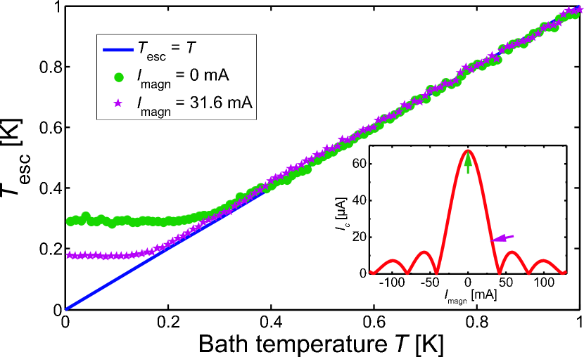
Figure 7: Calculated escape temperatures for sample B3 with and without an applied magnetic field. The inset shows the $I_{c}(\Phi)$ modulation of this junction; the arrows indicate where the MQT data was obtained. For $I_{\mathrm{magn}}=31.6\,$mA, a clear reduction of the observed crossover temperature $T_{\mathrm{cr}}$ is observed.

We now turn to the investigation of the crossover point from the thermal to the quantum regime and the influence of JJ size on it. As can be seen in Table 1, we expect a clear reduction of $T_{\mathrm{cr}}$ with increasing JJ size. However, an experimental observation of lower crossover temperatures for smaller JJs having smaller critical currents could simply be due to current noise in our measurement setup. In order to exclude this, we artificially reduced the critical current of sample B3 by applying a magnetic field in parallel to the junction area. While unwanted noise should now lead to an increase in the observed $T_{\mathrm{cr}}$, the physical expectation is a significantly reduced $T_{\mathrm{cr}}$ due to the lower plasma frequency according to (8). The result of this measurement can be seen in Fig. 7 and Table 4. We found an agreement between calculated and observed crossover temperature down to $T_{\mathrm{cr}}\approx 140$ mK, which was the lowest temperature we examined. Hence, it is clear that we have a measurement setup exhibiting low noise, where the electronic temperature is indeed equal to the bath temperature. The lowest investigated temperature of 140 mK is clearly below any temperature needed for the comparison of the JJs of different sizes with each other.

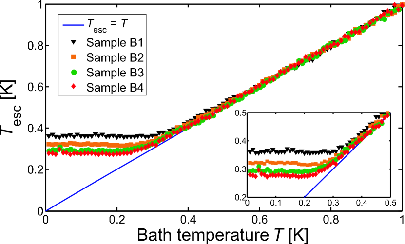
Figure 8: Calculated escape temperatures for all samples. The crossover to the quantum regime is very clear in each measurement. The inset shows a magnification of the quantum regime. The reduction of the crossover temperature $T_{\mathrm{cr}}$ with increasing JJ size is clearly visible.

Finally, we measured the switching histograms for the four JJs of different sizes and evaluated the escape temperature $T_{\mathrm{esc}}$ and the theoretical critical current $I_{c}$. This allowed us to determine the crossover temperature $T_{\mathrm{cr}}$ and the normalized crossover current $\gamma_{\mathrm{cr}}=I_{\mathrm{sw,cr}}/I_{c}$. We indeed found a clear dependence of the crossover temperature on the JJ size as can be seen in Fig. 8. To compare the experimental $\gamma_{\mathrm{cr}}$ and $T_{\mathrm{cr}}$ values with the ones expected by theory, we now performed the theoretical calculation described above using the experimentally determined $Q$ values and equation (13). All experimentally determined values are in excellent agreement with theory, as can be seen in Table 4.

Table 4: The experimentally determined values characterizing the crossover from the thermal to the quantum regime in comparison with the theoretical expectations for all measurements.

Sample	$I_{c}(\Phi)/I_{c}(0)$	$\gamma_{\mathrm{cr,theo}}$	$\gamma_{\mathrm{cr,exp}}$	$T_{\mathrm{cr,}Q\mathrm{,theo}}$	$T_{\mathrm{cr,exp}}$
				(mK)	(mK)
B-1	$1$	$0.965$	$0.970$	$368$	$362$
B-2	$1$	$0.977$	$0.981$	$322$	$321$
B-3	$1$	$0.988$	$0.990$	$290$	$294$
B-3	$0.52$	$0.984$	$0.987$	$223$	$236$
B-3	$0.27$	$0.979$	$0.983$	$172$	$176$
B-3	$0.13$	$0.973$	$0.975$	$129$	$147$
B-4	$1$	$0.988$	$0.990$	$276$	$278$

VI Conclusions

We have carried out systematic Macroscopic Quantum Tunneling (MQT) experiments with varying Josephson junction area. Our samples were fabricated on the same chip. Thorough characterization before the actual quantum measurements revealed that the junctions exhibit a very high quality. We showed that we could significantly decrease the damping at frequencies relevant for MQT by using lumped element inductors, which allowed us to perform our study in the low damping limit. The crossover from the thermal to the quantum regime was found to have a clear and systematic dependence on junction size, which is in perfect agreement with theory.