Variational and symplectic approach of the model-free control

Loïc MICHEL

GRÉI - Département de génie électrique et génie informatique
Université du Québec à Trois-Rivières
C.P. 500, Trois-Rivières, G9A 5H7, Canada, QC

Abstract

We propose a theoretical development of the model-free control in order to extend its robustness capabilities. The proposed method is based on the auto-tuning of the model-free controller parameter using an optimal approach. Some examples are discussed to illustrate our approach.

1 Introduction

The model-free control methodology, originally proposed by [1], has been widely successfully applied to many mechanical and electrical processes. The model-free control provides good performances in disturbances rejection and an efficient robustness to the process internal changes. To improve the efficiency of the model-free control, we propose to use the variational optimization principle in order to tune on-line the model-free control parameter $\alpha$.

The proposed approach considers the model-free control law as a cost criterion which could be minimized relating to the parameter $\alpha$. To minimize the cost criteria, the variational calculus is used considering properties of the symplectic geometry. In particular, it has been shown that the integration of a cost criteria under symplectic geometry assumptions provides very simple integration algorithms that can preserve physical properties of the integrated system and good convergence properties. Moreover, simplicity of this kind of integrator allows building an on-line optimization process that can adjust the $\alpha$ parameter according to the controlled process dynamic.

The paper is structured as follows. Section II presents an overview of the model-free control methodology including its advantages in comparison with classical methodologies. Section III discusses the application of the calculus of variations to the model-free control. Some concluding remarks may be found in Section IV.

2 Model-free control: a brief overview

2.1 General principles

2.1.1 The ultra-local model

We only assume that the plant behavior is well approximated in its operational range by a system of ordinary differential equations, which might be highly nonlinear and time-varying. The system, which is SISO, may be therefore described by the input-output equation

$$E(t,y,\dot{y},\dots,y^{(\iota)},u,\dot{u},\dots,u^{(\kappa)})=0$$ (1)

where

• $u$ and $y$ are the input and output variables,

• $E$, which might be unknown, is assumed to be a sufficiently smooth function of its arguments.

Assume that for some integer $n$, $0<n\leq\iota$, $\frac{\partial E}{\partial y^{(n)}}\not\equiv 0$. From the implicit function theorem we may write locally

$$y^{(n)}=\mathfrak{E}(t,y,\dot{y},\dots,y^{(n-1)},y^{(n+1)},\dots,y^{(\iota)},u,\dot{u},\dots,u^{(\kappa)})$$

By setting $\mathfrak{E}=F+\alpha u$ we obtain the ultra-local model.

Definition 2.1

[1] If $u$ and $y$ are respectively the variables of input and output of a system to be controlled, then this system admits the ultra-local model defined by:

$$y^{(n)}=F+\alpha u$$ (2)

where

• $\alpha\in\mathbb{R}$ is a non-physical constant parameter, such that $F$ and $\alpha u$ are of the same magnitude;

• the numerical value of $F$, which contains the whole “structural information”, is determined thanks to the knowledge of $u$, $\alpha$, and of the estimate of the derivative $y^{(n)}$.

In all the numerous known examples it was possible to set $n=1$ or $2$.

2.1.2 Numerical value of $\alpha$

Let us emphasize that one only needs to give an approximate numerical value to $\alpha$. It would be meaningless to refer to a precise value of this parameter.

2.2 Intelligent PI controllers

2.2.1 Generalities

Definition 2.2

[1] If $n=1$, we close the loop via the intelligent PI controller, or i-PI controller,

$$u=-\frac{F}{\alpha}+\frac{\dot{y}^{\ast}}{\alpha}+\mathcal{C}(\varepsilon)$$ (3)

where

• $y^{\ast}$ is the output reference trajectory, which is determined via the rules of flatness-based control ([3, 4]);

• $e=y^{\ast}-y$ is the tracking error;

• $\mathcal{C}(\varepsilon)$ is of the form $K_{P}\varepsilon+K_{I}\int\varepsilon$. $K_{P}$, $K_{I}$ are the usual tuning gains.

Equation (3) is called model-free control law or model-free law.

The i-PI controller 3 is compensating the poorly known term $F$. Controlling the system therefore boils down to the control of a precise and elementary pure integrator. The tuning of the gains $K_{P}$ and $K_{I}$ becomes therefore quite straightforward.

2.2.2 Classic controllers

See [5] for a comparison with classic PI controllers.

2.2.3 Applications

See [6, 7, 8, 9, 10, 11, 12, 13] for already existing applications in various domains.

2.3 Numerical differentiation of noisy signals

Numerical differentiation, which is a classic field of investigation in engineering and in applied mathematics, is a key ingredient for implementing the feedback loop 3. Our solution has already played an important role in model-based nonlinear control and in signal processing (see [14] for further details and related references).

The estimate of the $1^{st}$ order derivative of a noisy signal $y$ reads (see, e.g., [15]) $\hat{\dot{y}}=-\frac{3!}{T^{3}}\int^{T}_{0}(T-2t)y(t)dt$ where [0,T] is a quite “short” time window. This window is sliding in order to get this estimate at each time instant.

Denoising of $y$ leads to the estimate $\hat{y}=\frac{2!}{T^{2}}\int^{T}_{0}(2T-3t)y(t)dt$

The above results are the basis of our estimation techniques. Important theoretical developments, which are of utmost importance for the computer implementation, may be found in [16]. We establish the following hypothesis:

Hypothesis 2.1

[2] The estimate of the derivative is realized with an high bandwidth and is not biased; in particular compared to the noise.

2.4 A first academic example: a stable monovariable linear system

Introduce as in [1, 2] the stable transfer function

$$\frac{(s+2)^{2}}{(s+1)^{3}}$$ (4)

2.4.1 A classic PID controller

We apply the well known method due to Broïda (see, e.g., [17]) by approximating System 4 via the following delay system

$$\frac{Ke^{-\tau s}}{(Ts+1)}$$

$K=4$, $T=2.018$, $\tau=0.2424$ are obtained thanks to graphical techniques. The gain of the PID controller are then deduced [17]: $K_{P}=\frac{100(0.4\tau+T)}{120K\tau}=1.8181$, $K_{I}=\frac{1}{1.33K\tau}=0.7754$, $K_{D}=\frac{0.35T}{K}=0.1766$.

2.4.2 i-PI.

We are employing $\dot{y}=F+u$ and the i-PI controller

$$u=-[F]_{e}+\dot{y}^{\star}+\mathcal{C}(\varepsilon)$$

where

• $[F]_{e}=[\dot{y}]_{e}-u$,

• $y^{\star}$ is a reference trajectory,

• $\varepsilon=y^{\star}-y$,

• $\mathcal{C}(\varepsilon)$ is an usual PI controller.

2.4.3 Numerical simulations

Figure 1(a) shows that the i-PI controller behaves only slightly better than the classic PID controller (Fig. 1(b)). When taking into account on the other hand the ageing process and some fault accommodation there is a dramatic change of situation: Figure 1(c) indicates a clear cut superiority of our i-PI controller if the ageing process corresponds to a shift of the pole from $1$ to $1.5$, and if the previous graphical identification is not repeated (Fig. 1(d)).

2.4.4 Some consequences

• It might be useless to introduce delay systems of the type

  $$T(s)e^{-Ls},\quad\leavevmode\nobreak\ T\in{\mathbb{R}}(s),\leavevmode\nobreak\ L\geq 0$$ (5)

  for tuning classic PID controllers, as often done today in spite of the quite involved identification procedure.

• This example demonstrates also that the usual mathematical criteria for robust control become to a large irrelevant.

• As also shown by this example some fault accommodation may also be achieved without having recourse to a general theory of diagnosis.

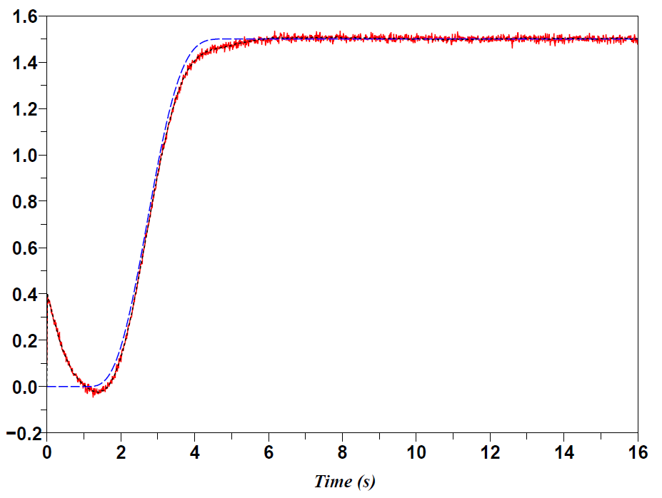
(a) i-PI control

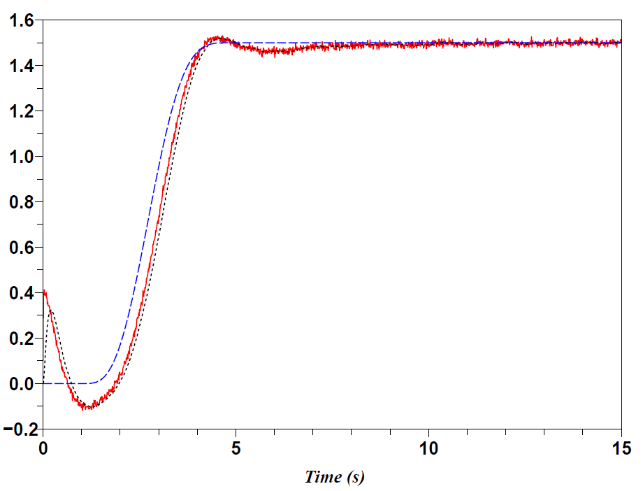
(b) PID control

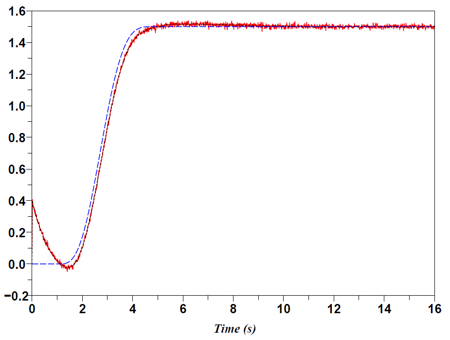
(c) i-PI control

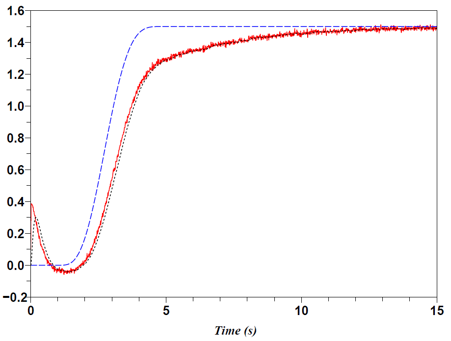
(d) PID control

Figure 1: Stable linear monovariable system (Output (–); reference (- -); denoised output (. .)).

2.5 From the analytical mechanics to the model-free control

The concept of symplecticity, described very largely by [18] gives a rigorous mathematical framework to the variational problems including the concept of symmetry. Lagrangian mechanics besides is completely formalized thanks to variational calculation within the framework of the symplectic spaces properties. It introduces, for the mechanical systems, the concept of Hamiltonian and the generalized coordinates $p$ and $q$ (resp. proportional to the position and the acceleration), which using the Euler-Lagrange equation and the Hamilton-Jacobi equation, allows to retrieve the basic principle of dynamics. Thus, in the case of a conservative mechanical system independent of time, the Hamiltonian energy is preserved and induces the conservation of certain properties in symplectic spaces [19]. Although the symplecticity is a relatively abstract concept, much of the works (let us quote e.g. [19, 20, 21, 22, 23, 24, 25]) established the possibility of using symplectic integration algorithms under certain conditions i.e able to preserve the Lagrangian structure of the mechanical systems, and to preserve the Hamiltonian in particular in the case of the systems that are independent of time.

3 Introduction to the variational model-free control

3.1 Possibility of controlling $\alpha$

The fundamental goal of a variational optimization of the model-free control law (3) is to increase the robustness/the tracking of the reference by an online adjustment of the parameter $\alpha$. Starting from the definition of a cost criterion, we justify the use of variational methods by the fact that they allow to calculate the parameter $\alpha$ as a solution of the optimization problem according to the time.

Considered application Consider an application in power electronics [13] where we have to control the output voltage of a power converter according to an output reference. Consider the dc/dc buck converter (Fig. 2) where $u$ is the duty-cycle and $E=20V$ $L=1$ mH, $C=10$ $\mu$F. The load is a simple varying resistor $R$.

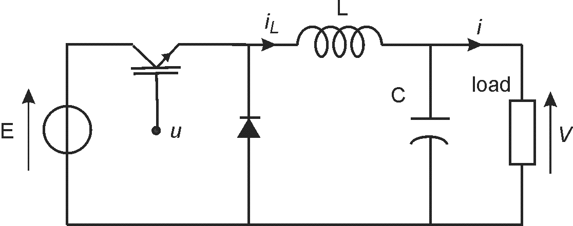
Figure 2: Classical buck converter.

$u$ is the input of the converter to control. The controlled output voltage is noted $y$ and the output reference voltage is noted $y^{*}$. The equivalent transfer function $H=y/u$ of this buck converter to control is of the second order and is stable.

3.2 Discrete model-free control law and associated properties

In practice, when the implementation of a i-PI controller is carried out in a digital way like a micro-controller or FPGA for example, it is necessary to discretize the i-PI controller of the def. (2.2).

$$u_{k}=-\frac{1}{\alpha}\left(F_{k-1}-\left.{y}^{(n)\ast}\right|_{k}\right)+\left.\mathcal{C}(\varepsilon)\right|_{k}=-\frac{1}{\alpha}\left(\underbrace{\left.{y}^{(n)}\right|_{k-1}-\alpha u_{k-1}}_{F_{k-1}}-\left.{y}^{(n)\ast}\right|_{k}\right)+\left.\mathcal{C}(\varepsilon)\right|_{k}$$ (6)

$${u_{k}=u_{k-1}-\frac{1}{\alpha}\left(\left.{y}^{(n)}\right|_{k-1}-\left.{y}^{(n)\ast}\right|_{k}\right)+\left.\mathcal{C}(\varepsilon)\right|_{k}}$$ (7)

Definition 3.1

For any discrete moment $t_{k},\,k\in\mathbb{N}$, one defines the discrete controller i-PI.

$$u_{k}=u_{k-1}-\frac{1}{\alpha}\left(\left.{y}^{(n)}\right|_{k-1}-\left.{y}^{(n)\ast}\right|_{k}\right)+\left.\mathcal{C}(\varepsilon)\right|_{k}$$ (8)

where

• $y^{\ast}$ is the output reference trajectory;

• $\varepsilon=y^{\ast}-y$ is the tracking error;

• $\mathcal{C}$ is a usual corrector PI where $K_{P}$, $K_{I}$ are the usual tuning gains.

The discrete intelligent controller is also called discrete model-free control law or discrete model-free law.

Theorem 3.1

[26] If the function $f(x,t)$ in the equation $\dot{x}=f(x,t)$ is continuous in $t$ and if it exists a positive constant $l$ such that:

$$||f(x_{2},t)-f(x_{1},t)||\leq l||x_{2}-x_{1}||$$ (9)

for all $x_{1}$ and $x_{2}$ in the neighborhood $\mathcal{B}_{r}$ of the origin, and for all $t\in[t_{0},t_{0}+T],T\in\mathbb{R}_{+}$, then the differential equation has a single solution $x(t)$ for sufficiently small initial states and a sufficiently short time period $T$. The condition (9), is called Lipschitz condition and the constant $l$ is the Lipschitz constant. If (9) is satisfied, one says that $f$ is locally Lipschitz.

The example presented Fig. 4 shows, in the case of a variable reference with a load disturbance, which occurs at (t = 0,003 s), and a simple corrector gain $K_{p}$, the existing difference between a model-free control law with $\alpha$ constant and $\alpha$ dependent on the time.

Hypothesis 3.1

The output reference voltage is $K_{y^{*}}$-Lipschitz and varies slowly according to the time.

The hyp. 3.1 implies that $u$ and thus $y$ and $\varepsilon$ are Lipschitz if the model-free control law is stable. In the same manner, it is appropriate to limit the variations on the possible drifts of the model $H$.

Hypothesis 3.2

The drifts of the $H$ parameters are Lipschitz.

In previous model-free control applications (e.g. [13]), the static value of $\alpha$ does not influence significantly the stability of the model-free control. However, when $\alpha$ varies, it proves that it is possible to act on the performances of the model-free control by adjusting on-line the $\alpha$ parameter. The objective is thus to be able to define a variation law of $\alpha$ such that the dynamic performances of the model-free control are improved.

3.2.1 Model-free control $\nu$-$K_{\alpha}$ degenerated

In order to assume correctly the variations of $\alpha$ within the discrete model-free law (8) and with an aim of satisfying the integration conditions of the Euler-Lagrange equation, which will allow the $\alpha$-optimization of the model-free law, it is advisable to define the dynamic of $\alpha$. Consequently, we consider the addition of the $\alpha$ derivative in (8).

Definition 3.2

When the system works in closed-loop, one defines the $u_{k}$-degenerate model-free law for $n=1$ such that:

$$u_{k}=u_{k-1}-\gamma\left(\left.\frac{\mathrm{d}y}{\mathrm{d}t}\right|_{k-1}-\left.\frac{\mathrm{d}y_{c}}{\mathrm{d}t}\right|_{k}\right)+\left.\mathcal{C}(\varepsilon)\right|_{k}+\left\{K_{\alpha}\left(\frac{\mathrm{d}\gamma}{\mathrm{d}t}\right)^{\nu}\right\}$$ (10)

where $\gamma=1/\alpha^{-\nu}$, $K_{\alpha}\in\mathbb{R}^{*}$ and $\nu\in\mathbb{N}$ that define the dynamics of variation of $\alpha$. The parameter $\alpha$ verifies the def. 2.1.

The model-free law (10) seems to be a redefinition of the original concept (2.2) taking into account the variations of the parameter $\alpha$.

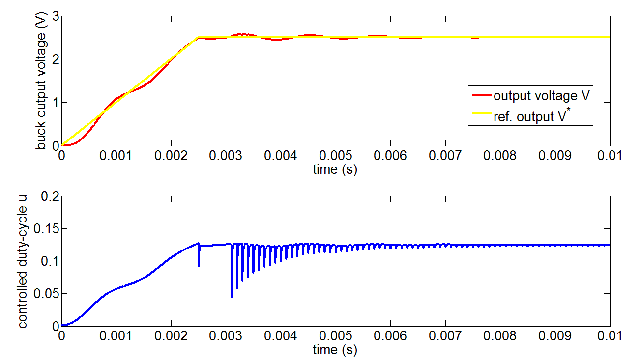
(a) $\alpha=14$, $K_{p}=2$

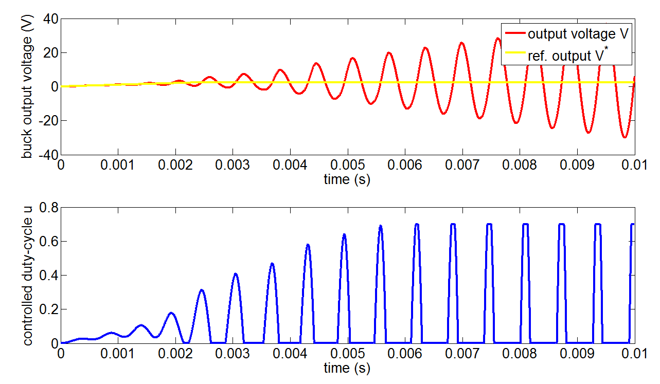
(b) $\alpha(t)=14+10^{6}\,t$, $K_{p}=2$

Figure 3: Comparison between $\alpha$ constant and $\alpha$ variable.

3.2.2 Model-free local control law $u_{k}$-implicite

We establish a non-recursive expression and implicitly dependant on $F$. According to the def. 2.2, and under the hyp. 2.1, we have in the discrete time:

$$u_{k}=-\frac{1}{\alpha^{-\nu}}\left(F_{k-1}-\left.\frac{\mathrm{d}y_{c}}{\mathrm{d}t}\right|_{k}\right)+\left\{K_{\alpha}\left(\frac{\mathrm{d}\gamma}{\mathrm{d}t}\right)^{\nu}\right\}+\left.\mathcal{C}(\varepsilon)\right|_{k}$$ (11)

that can be rewritten:

$$\alpha^{-\nu}u_{k}=-F_{k-1}+\left.\frac{\mathrm{d}y_{c}}{\mathrm{d}t}\right|_{k}+\alpha^{-\nu}\left\{K_{\alpha}\left(\frac{\mathrm{d}\gamma}{\mathrm{d}t}\right)^{\nu}\right\}+\alpha^{-\nu}\left.\mathcal{C}(\varepsilon)\right|_{k}$$ (12)

$$\alpha^{-\nu}u_{k}+F_{k-1}=\left.\frac{\mathrm{d}y_{c}}{\mathrm{d}t}\right|_{k}+\alpha^{-\nu}\left\{K_{\alpha}\left(\frac{\mathrm{d}\gamma}{\mathrm{d}t}\right)^{\nu}\right\}+\alpha^{-\nu}\left.\mathcal{C}(\varepsilon)\right|_{k}$$ (13)

According to the th. 3.1, we call, $u_{k}$-implicite model-free discrete law, the following expression:

$$\left.\underbrace{\frac{\mathrm{d}y}{\mathrm{d}t}}_{F_{k-1}+\alpha^{-\nu}u_{k-1}}\right|_{k-1}-\left.\frac{\mathrm{d}y_{c}}{\mathrm{d}t}\right|_{k}=\left.\alpha^{-\nu}\mathcal{C}(\varepsilon)\right|_{k}+\alpha^{-\nu}\left\{K_{\alpha}\left(\frac{\mathrm{d}\gamma}{\mathrm{d}t}\right)^{\nu}\right\}$$ (14)

$$\left.\frac{\mathrm{d}\varepsilon}{\mathrm{d}t}\right|_{k-1}=\left.\alpha^{-\nu}\mathcal{C}(\varepsilon)\right|_{k}+\alpha^{-\nu}\left\{K_{\alpha}\left(\frac{\mathrm{d}\gamma}{\mathrm{d}t}\right)^{\nu}\right\}$$ (15)

Let us define $\frac{\mathrm{d}\varepsilon}{\mathrm{d}t}=\left.\frac{\mathrm{d}y}{\mathrm{d}t}\right|_{k-1}-\left.\frac{\mathrm{d}y_{c}}{\mathrm{d}t}\right|_{k}$ like the derivative of the tracking error using the th. 3.1 via the hyp. 3.2.

When the corrector $\mathcal{C}$ is defined by a single constant gain $\mathcal{C}\equiv K_{p}$, then it exists a linear relation between $\alpha$ and the output and its derivative. It comes then:

Definition 3.3

The model-free Lagrangian verifies:

$$\frac{1}{K_{p}}\left\{\gamma\left.\frac{\mathrm{d}\varepsilon}{\mathrm{d}t}\right|_{k-1}+K_{\alpha}\left(\frac{\mathrm{d}\gamma}{\mathrm{d}t}\right)^{\nu}\right\}=\left.\varepsilon\right|_{k}$$ (16)

with $\gamma=\frac{1}{\alpha^{-\nu}}\in\mathbb{R}^{\ast}_{+}\qquad K_{p}\in\mathbb{R}^{\ast}_{+}\qquad K_{\alpha}\in\mathbb{R}^{*}\qquad\nu\in\mathbb{N}$

In this expression, the parameters $K_{p}$ and $K_{\alpha}$ are constants. Since the variable to find is $\gamma$, $\varepsilon$ and $\frac{\mathrm{d}\varepsilon}{\mathrm{d}t}$ are considered as constants over a small time.

3.3 Model-free Lagrangian

3.3.1 Criterion $L_{\alpha}$

Based on the $\nu$-$K_{\alpha}$-degenerated expression, we define the variational model-free criterion $L_{\alpha}$ such that:

$$L_{\alpha}=\int(y-y^{*})\mathrm{d}\tau=\int\frac{1}{K_{p}}\left\{\gamma\left.\frac{\mathrm{d}\varepsilon}{\mathrm{d}t}\right|_{k-1}+K_{\alpha}\left(\frac{\mathrm{d}\gamma}{\mathrm{d}t}\right)^{\nu}\right\}\mathrm{d}\tau$$ (17)

The expression $\nu$-$K_{\alpha}$-degenerated provides a ”direct equivalence relation” between the traditional expression of the reference tracking $y-y^{*}$ and the model-free control. The correction gain $K_{p}$ is here a scaling factor.

3.3.2 Elements of variational calculation

The fundamental theorem of calculus of variation defines the existence of a solution to the problem of integrals of functions minimization via the resolution of the Euler-Lagrange equation.

Theorem 3.2

The Euler-Lagrange equation [27]: Let $J:C^{2}[x_{0},x_{1}]\rightarrow\mathbb{R}$, be a functional of the form:

$$J(y)=\int_{x_{0}}^{x_{1}}f(x,y,y^{\prime})dx$$ (18)

where $f$ has continuous partial derivatives of second order with respect to $x$, $y$ and $y^{\prime}$, and $x_{0}<x_{1}$. Let:

$$S=\{y\in C^{2}[x_{0},x_{1}]:y(x_{0})=y_{0}\hbox{ et }y(x_{1})=y_{1}\}$$ (19)

where $y_{0}$ and $y_{1}$ are given real numbers. If $y\in S$ is an extremal for $J$, then

$$\frac{\mathrm{d}}{\mathrm{d}x}\left(\frac{\partial f}{\partial y^{\prime}}\right)-\frac{\partial f}{\partial y}=0$$ (20)

for all $x\in[x_{0},x_{1}]$.

The Euler-Lagrange equation, is thus a differential equation, generally nonlinear, that must be satisfied for any extremal function $y(x)$. In other words, if $y(x)$ is solution of the Euler-Lagrange equation, then the functional $J$, defined as the integral on $[x_{0},x_{1}]$ of a $f$, functional dependant on $x$, $y$ and $y^{\prime}$, is minimal.

3.3.3 Numerical resolution of the criterion $L_{\alpha}$

Conjecture 3.1

Under certain conditions to define, the Euler-Lagrange equation, applied to the variational model-free Lagrangian (17), establishes the possibility of controlling the tracking error $y-y^{*}$ permanently by the on-line adjustment of $\alpha$.

The Euler-Lagrange equation thus allows to determine $\alpha$ such that the criterion $L_{\alpha}$ is miminum. The continuous Euler-Lagrange reads:

$$\frac{\mathrm{d}}{\mathrm{d}t}\left(\frac{\partial L_{\alpha}}{\partial\alpha^{\prime}}\right)=\frac{\partial L_{\alpha}}{\partial\alpha}$$ (21)

The integration of the variational model-free Lagrangian (16) provides the evolution law of $\alpha$ according to the time such that the integral of the error $y-y^{*}$ is minimal.

Let us define the discrete Euler-Lagrange equation according to [28] [29] where $D_{1}$ and $D_{2}$ indicate the discrete derivation of the Lagrangian:

$$D_{2}L_{d}(\alpha_{k-1},\alpha_{k},h)+D_{1}L_{d}(\alpha_{k},\alpha_{k+1},h)=0$$ (22)

We have:

$$\frac{\nu}{K_{p}}\left\{\gamma_{k}\frac{\mathrm{d}\varepsilon}{\mathrm{d}t}+K_{\alpha}\frac{\gamma_{k-1}-\gamma_{k}}{h^{\nu}}\right\}+\frac{\nu}{K_{p}}\left\{\gamma_{k}\frac{\mathrm{d}\varepsilon}{\mathrm{d}t}+K_{\alpha}\frac{\gamma_{k+1}-\gamma_{k}}{h^{\nu}}\right\}=0$$ (23)

then:

$$\gamma_{k}\frac{\mathrm{d}\varepsilon}{\mathrm{d}t}+K_{\alpha}\frac{\gamma_{k+1}-2\gamma_{k}+\gamma_{k-1}}{h^{\nu}}=0$$ (24)

The discrete symplectic integrator derived from (24) is written (expression of $\gamma_{k+1}$ according to $\gamma_{K}$ and $\gamma_{k-1}$):

$$h^{\nu}\frac{\mathrm{d}\varepsilon}{\mathrm{d}t}\gamma_{k}+K_{\alpha}\left(\gamma_{k+1}-2\gamma_{k}+\gamma_{k-1}\right)=0$$ (25)

then:

$$\left(\frac{h^{\nu}}{K_{\alpha}}\frac{\mathrm{d}\varepsilon}{\mathrm{d}t}-2\right)\gamma_{k}+\gamma_{k-1}=-\gamma_{k+1}$$ (26)

Notice that the dependence with respect to the corrector $K_{p}$ does not exist anymore. Equation (10), called $\alpha$ control law forms with (16), the symplectic model-free control or i-PIS corrector (by extension of i-PI).

Definition 3.4

When the system works in closed-loop, we define the intelligent controller that is symplectic type or i-PIS controller by:

$$\begin{array}[]{l}\left\{\begin{array}[]{l}\displaystyle{u_{k}=u_{k-1}-\frac{1}{\alpha^{-n}}\left(\left.\frac{\mathrm{d}y}{\mathrm{d}t}\right|_{k-1}-\left.\frac{\mathrm{d}y_{c}}{\mathrm{d}t}\right|_{k}\right)+K_{p}\varepsilon\pm K_{\alpha}\left(\frac{\mathrm{d}\gamma}{\mathrm{d}t}\right)^{\nu}}\\ \displaystyle{-\left(\frac{h^{\nu}}{K_{\alpha}}\frac{\mathrm{d}\varepsilon}{\mathrm{d}t}-2\right)\gamma_{k}-\gamma_{k-1}=\gamma_{k+1}}\end{array}\right.\\ \gamma_{0}\,(resp.\,\alpha_{0})\,\hbox{ is initial condition}\end{array}$$ (27)

We preserved the natural notations of (10) (continuous into $\alpha$) and (16) (discrete form in $\alpha$ ). Let us note that $\alpha$ now seems a state variable of the model-free control.

Remarks

• instability of the strong load transients When there are disturbances (variations of model or load), the output may have to change quickly, this implies strong variations of the output derivative. However, under its conditions, although a Lipschitz condition is imposed on $\varepsilon$, the assumptions requested to apply the Euler-Lagrange equation may not be satisfied. Simulations of the § 3.5 show in particular that, if $R$ is varying very slowly, then at each level of $R$, $\alpha$ oscillates then is stabilized; more $R$ varies fast, more stabilization is slow.

• justification of the nature of (26) In order to interpret the form of the equation of the $\alpha$ control, which is of the damped harmonic oscillator type, let us look at the output buck converter signal in case of the i-PI (e.g. Fig. 5). Those appear naturally oscillating and the role of the derivative in (3) is to attenuate these oscillations in order to reach the permanent state. It thus appears rather intuitive that to counterbalance these oscillations, it would be enough to vary the coefficient $\alpha$ in the shape of an oscillator, which specifies well the law of $\alpha$ control.

• independence with respect to the initial condition on $\alpha$ the nature of the Euler-Lagrange equation implies a certain independence with respect to the initial conditions . This independence is in particular supposed to be true according to the simulations of the § 3.5. We can also conjecture that independence with respect to the $\alpha$ initial means that $\alpha$ is auto-adjusted even if it undergoes strong variations.

• critical integration step $h$ The integration step $h$ seems a critical element and must be selected sufficiently small to allow the preservation of the condition of integration of the th. 3.1.

3.4 Symplecticity of the numerical integration methods

Let us consider the damped mass system moving according to the $x$-coordinate for which we have the following Lagrangian:

$$L\left(x,\frac{\mathrm{d}x}{\mathrm{d}t}\right)=\frac{1}{2}m\left(\frac{\mathrm{d}x}{\mathrm{d}t}\right)^{2}+\frac{1}{2}kx^{2}$$ (28)

$m$ and $k$ are respectively the mass and the constant of the spring. Figures 4(a) and 4(b) present respectively the traditional response of the system according to the time and the comparison of the energy of (28) calculated via the different integration methods. This example shows that the symplectic integration of Euler, corresponding to the equation of $\alpha$ control (26) is at the same time easy to implement and efficient regarding the preservation of the energy.

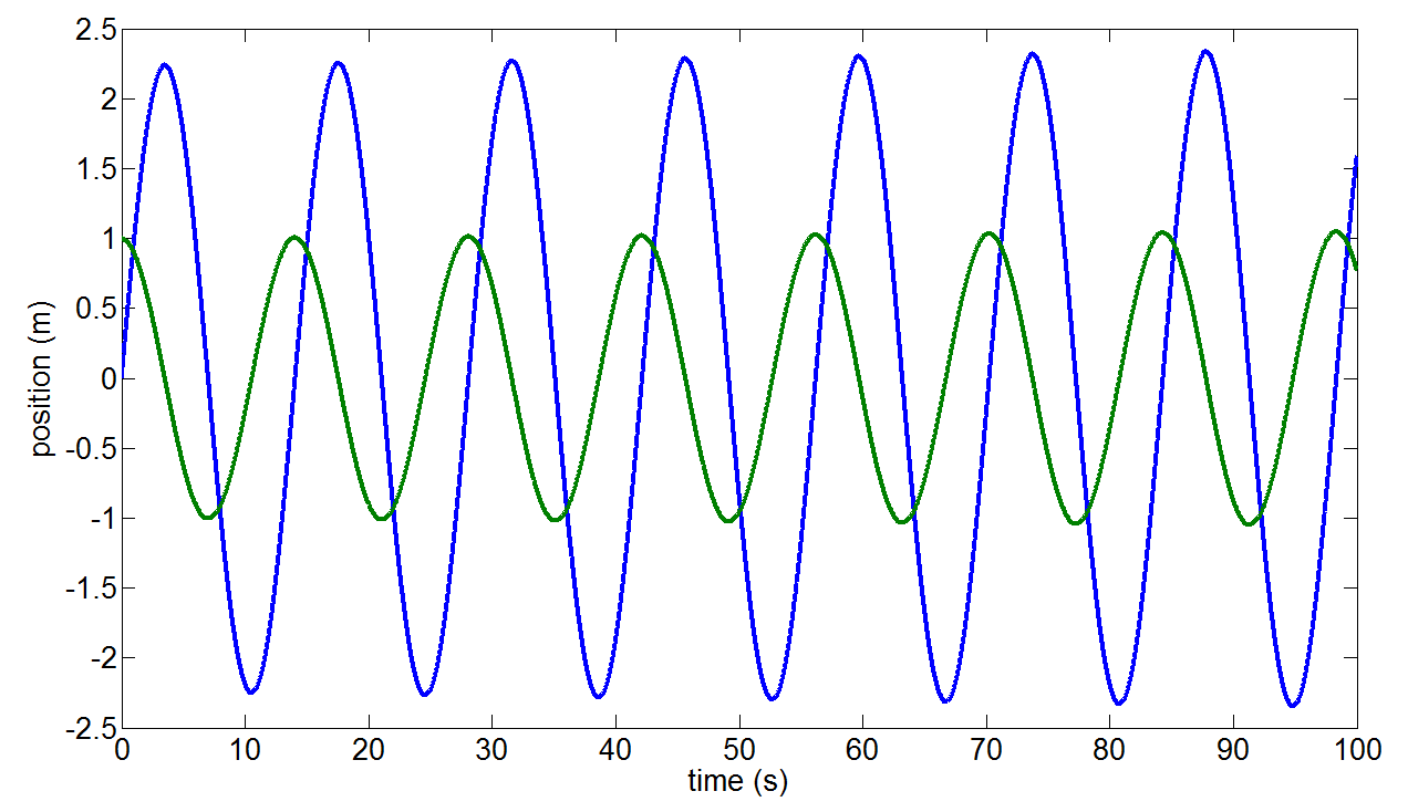
(a) Speed and position of the mass according to the time.

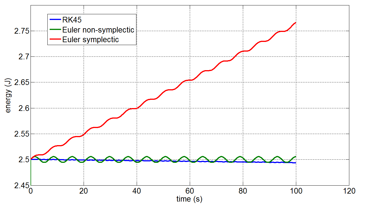
(b) Comparison of energy resulting from the various integration methods.

Figure 4: Symplectic integration.

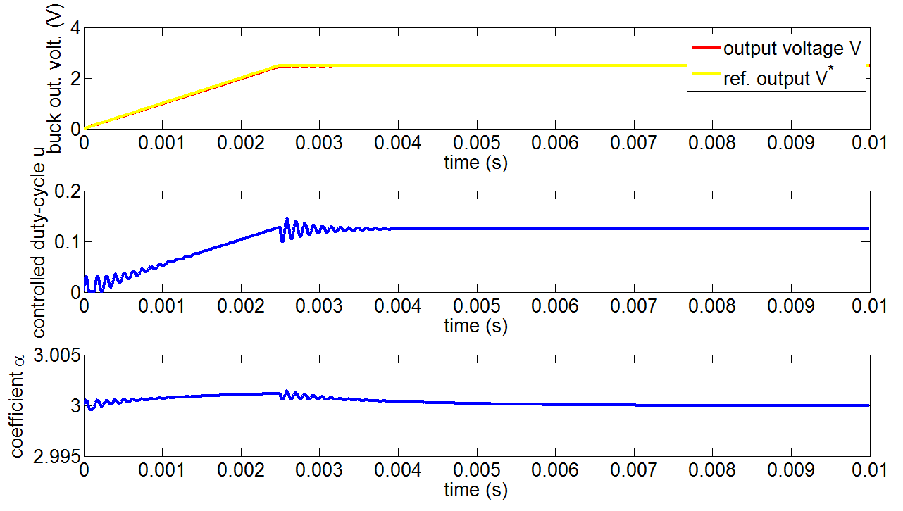
(a) i-PIS control for $\alpha_{0}=3$

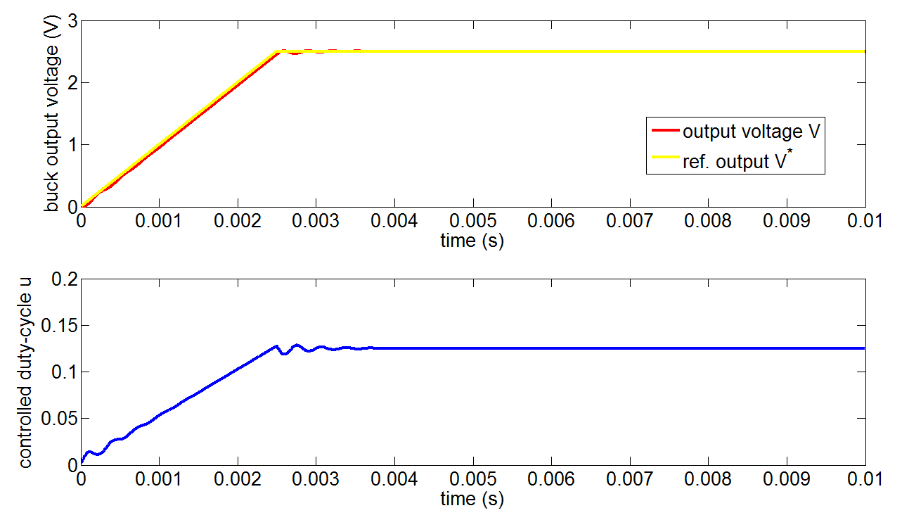
(b) i-PI control for $\alpha_{0}=3$

Figure 5: Comparison between i-PI and i-PIS without any load impact ($R$ does not change).

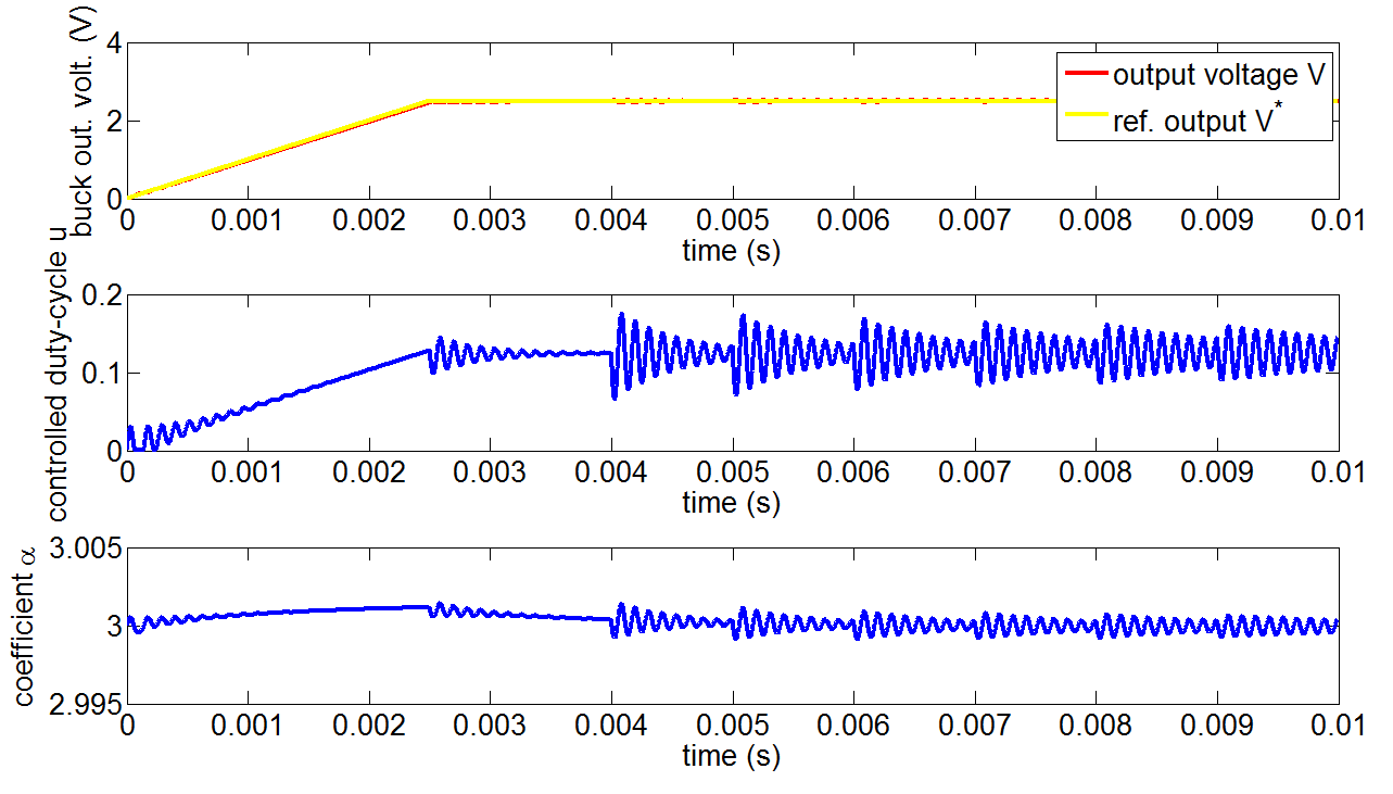
(a) $\alpha_{0}=3$

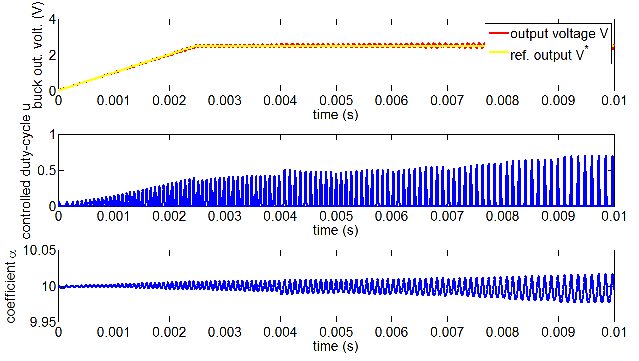
(b) $\alpha_{0}=10$

Figure 6: Comparison between two initial values of $\alpha$: the load resistor increases gradually from $R=10\Omega$ at $t=0,003$ s such that $R=18\Omega$ at $t=0,01$ s.

3.5 Application of the symplectic model-free control

Let us consider the buck converter for a slope output reference. Figure 5 presents the comparison between the i-PI and the i-PIS without impact of load; in all the cases, we took $\nu=1$ and $K_{\alpha}=2$. Let us note that the static error $\varepsilon$ tends to being slightly decreased in the case of the i-PIS, thanks to the ”harmonic” compensation of the $\alpha$ coefficient. Figure 6 presents the case of the i-PIS corrector for two initial values of $\alpha$ for a progressive impact of load of about 10 $\Omega$. Let us note that the variations of $\alpha$ allow a priori only an adjustment of the i-PIS sensitivity since the initial condition on $\alpha$ appears as a median value around which $\alpha$ is adjusted. It is thus advisable to be able to choose properly the initial value of $\alpha$.

Compared to the i-PIS corrector, one will note the importance of the Lipschitz condition in the stabilization of this kind of transient.

4 Towards a formalization of the model-free control?

We implemented a procedure of $\alpha$ auto-adjustment based on the calculus of variation and from the symplectic geometry considerations. The presented results are encouraging but there remain much of challenges before arriving to a completely optimal i-PIS form. Future work should be directed towards formal proofs of stability and dynamic performances.

References

- [1] M. Fliess and C. Join, “Commande sans modèle et commande à modèle restreint“, e-STA, vol. 5 (n∘ 4), pp. 1-23, 2008 (available at http://hal.inria.fr/inria-00288107/en/).
- [2] M. Fliess and C. Join, “Model-free control and intelligent PID controllers: Towards a possible trivialization of nonlinear control “, 15th IFAC Symp. System Identif., Saint-Malo, 2009 (available at http://hal.inria.fr/inria-00372325/en/).
- [3] M. Fliess, J. Lévine, P. Martin and P. Rouchon, “Flatness and defect of non-linear systems: introductory theory and examples“, Int. J. Control, vol. 61, pp. 1327-1361, 1995.
- [4] H. Sira-Ramírez and S. Agrawal, “Differentially Flat Systems“, Marcel Dekker, 2004.
- [5] B. d’Andréa-Novel, M. Fliess, C. Join, H. Mounier and B. Steux, “A mathematical explanation via “intelligent” PID controllers of the strange ubiquity of PIDs“, 18th Medit. Conf. Control Automation, Marrakech, 2010 (available at http://hal.inria.fr/inria-00480293/en/).
- [6] B. d’Andréa-Novel, C. Boussard, M. Fliess, O. El Hamzaoui, H. Mounier and B. Steux, “Commande sans modèle de vitesse longitudinale d’un véhicule électrique“, 6e Conf. Internat. Francoph. Automatique, Nancy, 2010 (available at http://hal.inria.fr/inria-00463865/en/).
- [7] S. Choi, B. d’Andréa-Novel, M. Fliess and H. Mounier, “Model-free control of automotive engine and brake for stop-and-go scenario“, 10th IEEE Conf. Europ. Control Conf., Budapest, 2009 (available at http://hal.inria.fr/index.php?halsid=1trv221lj8gke47u27bk03n2t6&view_this_doc=inria-00395393&version=1).
- [8] P.-A. Gédouin, C. Join, E. Delaleau, J.-M. Bourgeot, S. Arbab-Chirani and S. Calloch, “Model-free control of shape memory alloys antagonistic actuators“, 17th IFAC World Congress, Seoul, 2008 (available at http://hal.inria.fr/inria-00261891/en/).
- [9] P.-A. Gédouin, C. Join, E. Delaleau, J.-M. Bourgeot, S. Arbab-Chirani and S. Calloch, “A new control strategy for shape memory alloys actuators“, 8th Europ. Symp. Martensitic Transformations, Prague, 2009 (available at http://hal.inria.fr/inria-00424933/en/).
- [10] C. Join, J. Masse and M. Fliess, “Étude préliminaire d’une commande sans modèle pour papillon de moteur“, J. europ. syst. automat., vol. 42, pp. 337-354, 2008 (available at http://hal.inria.fr/inria-00187327/en/).
- [11] C. Join, G. Robert and M. Fliess, “Vers une commande sans modèle pour aménagements hydroélectriques en cascade“, 6e Conf. Internat. Francoph. Automat., Nancy, 2010 (available at http://hal.inria.fr/inria-00460912/en/).
- [12] J. Villagra and C. Balaguer, “Robust motion control for humanoid robot flexible joints“, 18th Medit. Conf. Control Automation, Marrakech, 2010.
- [13] L. Michel, C. Join, M. Fliess, P. Sicard and A. Chériti, “Model-free control of dc/dc converter“, in 2010 IEEE 12th Workshop on Control and Modeling for Power Electronics, pp.1-8, June 2010. (available at http://hal.inria.fr/inria-00495776/).
- [14] M. Fliess, C. Join and H. Sira-Ramírez, “Non-linear estimation is easy“, Int. J. Model. Identif. Control, vol. 4, pp. 12-27, 2008 (available at http://hal.inria.fr/inria-00158855/en/).
- [15] F.A. García Collado, B. d’Andréa-Novel, M. Fliess and H. Mounier, “Analyse fréquentielle des dérivateurs algébriques“, XXIIe Coll. GRETSI, Dijon, 2009 (available at http://hal.inria.fr/inria-00394972/en/).
- [16] M. Mboup, C. Join and M. Fliess, “Numerical differentiation with annihilators in noisy environment“, Numer. Algor., vol. 50, pp. 439-467, 2009.
- [17] D. Dindeleux, “Technique de la régulation industrielle“, Eyrolles, 1981.
- [18] J. Marsden and T.S. Ratiu, “Introduction to Mechanics and Symmetry: A Basic Exposition of Classical Mechanical Systems“. Springer, 1 January 1999.
- [19] R.J. O’Neale, “Preservation of phase space symplectic structure in symplectic integration“, Ph.D. dissertation thesis, Massey University, New Zeland, 2009.
- [20] M. Leok, “Foundations of Computational Geometric Mechanics“, Ph.D. dissertation thesis, California Institute of Technology, CA, 2004.
- [21] A.M. Bloch, N.E. Leonard, J.E. Marsden, “Controlled Lagrangians and the stabilization of mechanical systems. I. The first matching theorem“, IEEE Transactions on Automatic Control, vol.45, no.12, pp.2253-2270, Dec. 2000.
- [22] A.M.Bloch, Eui Chang Dong ; N.E. Leonard and J.E. Marsden , “Controlled Lagrangians and the stabilization of mechanical systems. II. Potential shaping“, IEEE Transactions on Automatic Control, vol.46, no.10, pp.1556-1571, Oct 2001.
- [23] J. E. Marsden, S. Pekarsky, S. Shkoller and M. West, “Variational methods, multisymplectic geometry and continuum mechanics“, Journal of Geometry and Physics, Volume 38, Issues 3-4, pp. 253-284, June 2001.
- [24] A. N. Hirani, “Linearization methods for variational integrators and Euler-Lagrange equations“, Master thesis, California Institute of Technology, 2000.
- [25] J.E. Marsden and M. West, “Discrete mechanics and variational integrators“, Acta Numerica 10, pp.357-514, 2001.
- [26] J.-J E. Slotine and W. Li, “Applied nonlinear control“, Prentice-Hall, 1991.
- [27] B. Van Brunt, “The calculus of variations“, Ed. Springer, 2006.
- [28] G. Vilmart, “Étude d’intégrateurs géométriques pour des équations différentielles“, Ph.D. dissertation thesis, École Normale Supérieure de Cachan, France, 2008.
- [29] M. West, “Variational integrators“, Ph.D. dissertation thesis, California Institute of Technology, CA, 2004.