Leading order hadronic contribution to g-2 from twisted mass QCD

Abstract:

We calculate the leading order hadronic contribution to the muon anomalous magnetic moment using twisted mass lattice QCD. The pion masses range from $330~{}\mathrm{MeV}$ to $650~{}\mathrm{MeV}$. We use two lattice spacings, $a=0.079~{}\mathrm{fm}$ and $0.063~{}\mathrm{fm}$, to study lattice artifacts. Finite-size effects are studied for two values of the pion mass, and we calculate the disconnected contributions for four ensembles. Particular attention is paid to the dominant contributions of the vector mesons, both phenomenologically and from our lattice calculation.

1 Introduction

A persistent discrepancy of about $3.2\,\sigma$ between the measured [1] and the theoretically calculated [2] anomalous magnetic moment of the muon, $a_{\mu}$, has motivated several lattice calculations of the leading order hadronic contribution, $\Delta\,a_{\mu}$ [3, 4, 5, 6, 7]. This contribution is the dominant source of error in the theoretical estimate of $a_{\mu}$ and presents both a challenge and opportunity for lattice QCD calculations. Here we extend our previous work [6] to address most of the systematic errors in an effort to establish what is required for a precise calculation of $\Delta\,a_{\mu}$. A detailed analysis will be presented elsewhere, so these proceedings will focus on the contributions of the vector mesons.

2 Leading order hadronic contribution to $a_{\mu}$

The leading order hadronic contribution to the anomalous magnetic moment of the muon can be calculated from the vacuum polarization tensor using the following expression from [3].

$$\Delta\,a_{\mu}=\alpha^{2}\int_{0}^{\infty}\!\!dQ^{2}\,\,\frac{1}{Q^{2}}w(Q^{2}/m_{l}^{2})\Pi_{R}(Q^{2})$$ (1)

The renormalized vacuum polarization function is $\Pi_{R}(Q^{2})=\Pi(Q^{2})-\Pi(0)$ and the weight function is given in [3]. The relevant lattice details for this calculation can be found in [6].

The hadronic correction to $a_{\mu}$ is normally estimated using a dispersion relation and experimental measurements of the cross section $\sigma(e^{+}e^{-}\rightarrow\mathrm{hadrons})$. A recent review [2] provides a list of results ranging from $\Delta\,a_{\mu}=684.6~{}(6.4)\cdot 10^{-10}$ to $711.0~{}(5.8)\cdot 10^{-10}$. The variation in the experimental estimates is beyond our current precision, so in the following we will use just the estimate of $691.0~{}(5.3)\cdot 10^{-10}$ from [8]. More important than the total value for $\Delta\,a_{\mu}$ are the individual contributions. The low energy region is dominated by the vector mesons: $\rho$, $\omega$ and $\phi$. The contributions from each are given in [8] as

$$\left.\Delta\,a_{\mu}\right|_{\rho}=501.1~{}(3.0)\cdot 10^{-10}~{}~{}~{}~{}\left.\Delta\,a_{\mu}\right|_{\omega}=37.0~{}(1.1)\cdot 10^{-10}~{}~{}~{}~{}\left.\Delta\,a_{\mu}\right|_{\phi}=34.42~{}(0.9)\cdot 10^{-10}\,.$$

Taken together, these three contributions already account for about $83\%$ of the total $\Delta\,a_{\mu}$. Verifying the contributions from the vector mesons is clearly a good first step towards calculating the complete $\Delta\,a_{\mu}$.

3 Vector mesons

As discussed in previous lattice calculations of $\Delta\,a_{\mu}$, the low $Q^{2}$ region of $\Pi_{R}(Q^{2})$ requires an interpolation and extrapolation in order to perform the integration in Eq. 1. Currently this requires introducing some model assumptions. Given the significant contributions of the lightest vector mesons, it is reasonable to incorporate their contributions into the $Q^{2}$ shape of the model. First we establish what is known regarding the electromagnetic decays of the $\rho$, $\omega$ and $\phi$. Then we discuss the additional model assumptions needed to calculate the contributions of the vector mesons to $\Delta\,a_{\mu}$.

3.1 Vector meson decay constants

The electromagnetic coupling of a vector meson is defined by

$$\langle\Omega|J^{em}_{\mu}(0)|V,p,\epsilon\rangle=m_{V}^{2}g_{V,em}\epsilon_{\mu}(p)~{}~{}~{}~{}~{}~{}~{}~{}f_{V,em}=m_{V}g_{V,em}\,.$$

The value of $g_{V,em}$ can be determined through the decay $V\rightarrow e^{+}e^{-}$. A straightforward exercise gives the partial width for this decay as

$$\Gamma(V\rightarrow e^{+}e^{-})=\frac{4\pi}{3}\alpha_{em}^{2}g^{2}_{V,em}m_{V}(1+2m_{e}^{2}/m_{V}^{2})\sqrt{1-4m_{e}^{2}/m_{V}^{2}}\,.$$

Using the latest values from the PDG [9], we find

$$g_{\rho,em}=0.20174\,(86)~{}~{}~{}~{}g_{\omega,em}=0.05863\,(98)~{}~{}~{}~{}g_{\phi,em}=0.07473\,(120)\,.$$

It is common to represent these decay constants in an isospin basis defined as

$$J^{I=0}_{\mu}=(\overline{u}\gamma_{\mu}u+\overline{d}\gamma_{\mu}d)/\sqrt{2}~{}~{}~{}~{}J^{I=1}_{\mu}=(\overline{u}\gamma_{\mu}u-\overline{d}\gamma_{\mu}d)/\sqrt{2}~{}~{}~{}~{}J^{s}_{\mu}=\overline{s}\gamma_{\mu}s\,.$$

Assuming $m_{u}=m_{d}$, $\phi$ is a pure $\overline{s}s$ state and $\omega$ has no $\overline{s}s$ contribution yields

$$f_{\rho}=\sqrt{2}f_{\rho,em}~{}~{}~{}~{}f_{\omega}=3\sqrt{2}f_{\omega,em}~{}~{}~{}~{}f_{\phi}=-3f_{\phi,em}\,$$

where $\langle\Omega|J_{\mu}|V,p,\epsilon\rangle=m_{V}f_{V}\epsilon_{\mu}(p)$ defines the isospin projected decay constants and the current is understood to correspond to the given meson. The resulting numerical values are

$$f_{\rho}=221.3\,(1.0)~{}\mathrm{MeV}~{}~{}~{}~{}f_{\omega}=194.7\,(3.2)~{}\mathrm{MeV}~{}~{}~{}~{}f_{\phi}=228.7\,(3.6)~{}\mathrm{MeV}\,,$$

which are all of the same order of magnitude. This is the expectation from chiral perturbation theory assuming precisely this pattern of $\omega$-$\phi$ mixing. Letting $f_{V}$ denote the generic vector meson decay constant in this case gives

$$f_{\rho,em}=\frac{f_{V}}{\sqrt{2}}~{}~{}~{}~{}f_{\omega,em}=\frac{f_{V}}{3\sqrt{2}}~{}~{}~{}~{}f_{\phi,em}=-\frac{f_{V}}{3}\,.$$

This can be generalized to include the $\omega$-$\phi$ mixing with an angle $\theta$, resulting in

$$f_{\rho,em}=\frac{f_{V}}{\sqrt{2}}~{}~{}~{}~{}f_{\omega,em}=\sin\theta\frac{f_{V}}{\sqrt{6}}~{}~{}~{}~{}f_{\phi,em}=-\cos\theta\frac{f_{V}}{\sqrt{6}}\,.$$

As needed shortly, we note that $\tan\theta=1/\sqrt{2}$ is the angle that corresponds to a pure $\overline{s}s$ state for the $\phi$ and this angle reduces the previous line to the line before.

3.2 Vector meson contributions to $\Delta\,a_{\mu}$

The couplings in the previous section are on-shell properties of the mesons, but now we must discuss the off-shell aspects of the vectors. This inevitably introduces a model dependence. Tree-level calculations in chiral perturbation theory provide a definite off-shell form of the vector meson propagator and give a contribution to the renormalized vacuum polarization function of

$$\Pi_{R,V}(Q^{2})=\frac{f_{V,em}^{2}}{m_{V}^{2}}\frac{Q^{2}}{Q^{2}+m_{V}^{2}}\,.$$

This expression can also be achieved by simply assuming an off-shell propagator of the form $A/(Q^{2}+m_{V}^{2})$ and fixing $A$ by demanding the correct $\Gamma(V\rightarrow e^{+}e^{-})$ result.

Combining the above result with the relationships between the decay constants gives

$$\Pi_{R,\rho+\omega+\phi}(Q^{2})=f_{V}^{2}\left\{\frac{1}{2}\frac{Q^{2}/m_{\rho}^{2}}{Q^{2}+m_{\rho}^{2}}+\frac{\sin^{2}\theta}{6}\frac{Q^{2}/m_{\omega}^{2}}{Q^{2}+m_{\omega}^{2}}+\frac{\cos^{2}\theta}{6}\frac{Q^{2}/m_{\phi}^{2}}{Q^{2}+m_{\phi}^{2}}\right\}\,.$$

Additionally setting $m_{\rho}=m_{\omega}=m_{\phi}=m_{V}$ gives

$$\Pi_{N_{f}=3}(Q^{2})=\frac{2f_{V}^{2}}{3m_{V}^{2}}\frac{Q^{2}}{Q^{2}+m_{V}^{2}}\,.$$

In the above we now make explicit that this is envisioned as a three-flavor result. We can also extract the two-flavor result by decoupling the $\phi$ and demanding a pure $\overline{s}s$ state for the $\phi$ by setting $\tan\theta=1/\sqrt{2}$. The resulting expression is

$$\Pi_{N_{f}=2}(Q^{2})=\frac{5f_{V}^{2}}{9m_{V}^{2}}\frac{Q^{2}}{Q^{2}+m_{V}^{2}}\,.$$

Notice that the strength of the $N_{f}=2$ and $3$ results follows the sum of the charges squared.

The resulting integral in Eq. 1 can be performed giving the following contributions for each of the vector mesons.

$$\Delta\,a_{\mu,\rho}=470.9.~{}(4.0)\cdot 10^{-10}~{}~{}~{}~{}\Delta\,a_{\mu,\omega}=39.1~{}(1.3)\cdot 10^{-10}~{}~{}~{}\Delta\,a_{\mu,\phi}=39.0~{}(1.3)\cdot 10^{-10}\,.$$

These values already reproduce much of the experimentally determined contributions given earlier. The discrepancy is largest for the $\rho$ and is a likely indicator of the effects of the $\rho\rightarrow\pi\pi$ decay.

4 Lattice calculation

$\beta$	$L/a$	$a\mu$	$m_{\pi}~{}[\mathrm{MeV}]$	$m_{V}~{}[\mathrm{MeV}]$	$f_{V}~{}[\mathrm{MeV}]$	$\Delta\,a_{\mu,V}~{}[10^{-10}]$
3.90	20	0.0040	347.9 (6.2)	1209. (161.)	345. (64.)	209. (45.)
3.90	24	0.0150	645.9 (1.7)	1235. (23.)	322. (10.)	164. (6.)
3.90	24	0.0100	524.5 (1.2)	1156. (36.)	312. (13.)	199. (11.)
3.90	24	0.0085	484.6 (1.2)	1144. (34.)	305. (13.)	198. (9.)
3.90	24	0.0064	423.1 (1.0)	1083. (35.)	297. (11.)	234. (15.)
3.90	24	0.0040	340.2 (1.7)	1067. (46.)	290. (15.)	237. (19.)
3.90	32	0.0040	334.2 (0.5)	1044. (51.)	296. (17.)	267. (26.)
3.90	32	0.0030	291.5 (1.0)	956. (70.)	260. (20.)	295. (45.)
4.05	24	0.0060	453.5 (3.4)	1094. (39.)	308. (14.)	241. (15.)
4.05	32	0.0080	517.1 (1.6)	1124. (36.)	298. (12.)	204. (13.)
4.05	32	0.0060	448.5 (1.9)	1104. (45.)	299. (17.)	219. (14.)
4.05	32	0.0030	325.1 (1.9)	1063. (78.)	297. (25.)	254. (35.)

Table 1: Ensembles and results used in this work. The pion masses are taken from [10] with one exception. The $L/a=20$ result was communicated privately by the ETMC collaboration. The lattice spacings are $a=0.079\,(2)~{}\mathrm{fm}$ and $0.063\,(1)~{}\mathrm{fm}$ for $\beta=3.90$ and $4.05$ [10]. Results from this work are the vector meson masses $m_{V}$, decay constants $f_{V}$ and the corresponding contribution to $\Delta\,a_{\mu}$ (the last two are normalized as the $\rho$ contribution). Up to disconnected contributions, the $N_{f}=2$ value of $\Delta\,a_{\mu}$ is $10/9$ of $\Delta\,a_{\mu,V}$. Additionally ignoring $s$ quark quenching effects, the $N_{f}=3$ value is $4/3$ of $\Delta\,a_{\mu,V}$.

The vector decay constant can be calculated from the correlator of the non-singlet current as follows.

$$\sum_{i}\int\!\!d^{3}\vec{x}\,\,\langle J^{I=1}_{i}(t,\vec{x})J^{I=1}_{i}(0)\rangle\rightarrow\frac{e^{-m_{V}t}}{2m_{V}}\sum_{\vec{\epsilon}}\langle\Omega|J_{i}|V,\vec{\epsilon}\rangle\langle V,\vec{\epsilon}|J_{i}|\Omega\rangle=\frac{3m_{V}f_{V}^{2}}{2}e^{-m_{V}t}$$

This correlator can be calculated on the lattice without disconnected diagrams. Let $C_{\mu\nu}(x)$ denote the connected piece of the single quark correlator $\langle J^{q}_{\mu}(x)J^{q}_{\nu}(0)\rangle$. Similarly let $D_{\mu\nu}(x)$ be the disconnected piece. Then the $I=1$ correlator is

$$\langle J^{I=1}_{\mu}(x)J^{I=1}_{\nu}(0)\rangle=C_{\mu\nu}(x)\,.$$

Additionally, the electromagnetic coupling of the $\rho$ can also be calculated directly without disconnected diagrams.

$$\langle J^{em}_{\mu}(x)J^{I=1}_{\nu}(0)\rangle=\frac{1}{\sqrt{2}}C_{\mu\nu}(x)$$

This is consistent with the earlier relationship $f_{\rho,em}=f_{\rho}/\sqrt{2}$.

The $\omega$ and $\phi$ decay constants are then obtained from

$$\langle J^{I=0}_{\mu}(x)J^{I=0}_{\nu}(0)\rangle=C_{\mu\nu}(x)+2D_{\mu\nu}(x)$$

and

$$\langle J^{s}_{\mu}(x)J^{s}_{\nu}(0)\rangle=C_{\mu\nu}(x)+D_{\mu\nu}(x)\,.$$

In the last expression we are assuming a quenched strange quark that is degenerate with the $u$ and $d$ quarks. Thus ignoring disconnected diagrams we find $m_{\omega}=m_{\phi}=m_{\rho}$ and $f_{\omega}=f_{\phi}=f_{\rho}$. The electromagnetic couplings can also be calculated using the following expressions.

$$\langle J^{em}_{\mu}(x)J^{I=0}_{\nu}(0)\rangle=\frac{1}{3\sqrt{2}}C_{\mu\nu}(x)+\frac{5}{3\sqrt{2}}D_{\mu\nu}(x)$$

$$\langle J^{em}_{\mu}(x)J^{s}_{\nu}(0)\rangle=-\frac{1}{3}C_{\mu\nu}(x)$$

Again we see that up to $s$ quark quenching effects and disconnected diagrams the results $f_{\omega,em}=f_{\omega}/(3\sqrt{2})$ and $f_{\phi,em}=-f_{\phi}/3$ are reproduced. This makes it clear that the theory with a quenched strange quark should be compared to the $\tan\theta=1/\sqrt{2}$ scenario in which the $\phi$ is pure $\overline{s}s$ state.

The full electromagnetic vacuum polarization function in the $N_{f}=2$ calculation is

$$\left.\langle J^{em}_{\mu}(x)J^{em}_{\nu}(0)\rangle\right|_{N_{f}=2}=\frac{5}{9}C_{\mu\nu}(x)+\frac{1}{9}D_{\mu\nu}(x)$$

and the result including a quenched and degenerate strange quark is

$$\left.\langle J^{em}_{\mu}(x)J^{em}_{\nu}(0)\rangle\right|_{N_{f}=3}=\frac{2}{3}C_{\mu\nu}(x)\,.$$

Again notice that, up to disconnected contributions and quenching effects, the $N_{f}=2$ and $3$ results agree to within the sum of charges squared.

5 Results

Our earlier calculation [6] has been extended to include a second lattice spacing, more quark masses, volumes and estimates of disconnected diagrams. (See Tab. 1.) Here we focus on the simplest model for $\Pi_{R}(Q^{2})$ that includes only the vector mesons. The vector meson masses and decay constants and the corresponding contribution to $\Delta\,a_{\mu}$ are given in Tab. 1. The vector contribution to $\Delta\,a_{\mu}$, normalized as the $\rho$, rises from $164~{}(6)\cdot 10^{-10}$ to $295~{}(45)\cdot 10^{-10}$ but falls well short of the expected $501.1~{}(3.0)\cdot 10^{-10}$.

We suspect that this discrepancy is mainly due to the large value of the $\rho$ mass found for the range of $\pi$ masses in Tab. 1. To illustrate this point, we plot the coupling of the vector meson in Fig. 2.

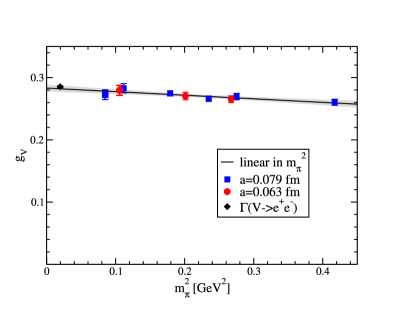
Figure 1: Vector coupling. The vector coupling, normalized as the $\rho$, calculated for $a=0.079~{}\mathrm{fm}$ and $a=0.063~{}\mathrm{fm}$ agree. A linear extrapolation in $m_{\pi}^{2}$ to the physical pion mass agrees with the value extracted from $\Gamma(V\rightarrow e^{+}e^{-})$. The factor of $m_{V}$ in $f_{V}$ hides this agreement.

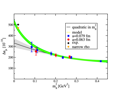
Figure 2: Vector contribution to $\Delta\,a_{\mu}$. A quadratic extrapolation in $m_{\pi}^{2}$ undershoots the measured contribution of the $\rho$ significantly. A model (described in text) suggests the importance of calculating at small enough $m_{\pi}$ for the vector mass to approach the physical $\rho$ mass.

There we see that $g_{V}$ appears to have a mild quark mass dependence and a simple linear extrapolation in $m_{\pi}^{2}$ gives a value in agreement with the experimental measurement. We can isolate the dependence of $\Delta\,a_{\mu,V}$ on $g_{V}$ and $m_{V}$ by integrating Eq. 1 exactly and then expanding in $m_{\mu}/m_{V}$. The first few terms are

$$\Delta\,a_{\mu,V}=2\alpha^{2}g_{V}^{2}\left(\frac{m_{\mu}}{m_{V}}\right)^{2}\left\{\frac{1}{3}+\frac{25}{12}\left(\frac{m_{\mu}}{m_{V}}\right)^{2}+\left(\frac{m_{\mu}}{m_{V}}\right)^{2}\ln\left(\frac{m_{\mu}}{m_{V}}\right)^{2}+{\cal O}\left(\frac{m_{\mu}}{m_{V}}\right)^{4}\right\}\,.$$

This makes it plausible that the discrepancy is simply due to the large value of the $\rho$ mass and the approach to the physical point should account for most of the discrepancy between the current values of $\Delta\,a_{\mu,V}$ and the experimental measurement. To illustrate this, we fit the chiral expansion $m_{V}=a+bm_{\pi}^{2}+cm_{\pi}^{3}$ to both our lattice results and also the physical value of the $\rho$ mass. Combining this with the fit to $g_{V}$ we produce the model curve in Fig. 2. Because $g_{V}$ extrapolates to the physical value and $m_{V}$ was constrained to give the physical $\rho$ mass, this model automatically reproduces the narrow $\rho$ approximation from earlier.

6 Conclusions

The final results of this work will be given in a forthcoming publication. Here we focus on understanding the dominant contribution from the vector mesons. Our current calculations produce values of $\Delta\,a_{\mu}$ that are significantly lower than the experimental measurements. We construct a model that suggests that this effect may be caused partially by a $\rho$ mass that is still rather large compared to its physical value. Thus we expect that calculations with the physical value of the $\pi$ mass and including the strange and charm quark contributions will be capable of achieving the precision necessary to match the accuracy of current experimental measurements of $\Delta\,a_{\mu}$.

7 Acknowledgments

We thank Carsten Urbach for his valuable collaboration, and we thank the John von Neumann Institute for Computing (NIC), the Jülich Supercomputing Center and the DESY Zeuthen Computing Center for their computing resources. This work has been supported in part by the DFG Sonderforschungsbereich/Transregio SFB/TR9-03 and the DFG project Mu 757/13 and is coauthored in part by Jefferson Science Associates, LLC under U.S. DOE Contract No. DE-AC05-06OR23177.

References

• [1] Muon G-2 Collaboration. Final Report of the Muon E821 Anomalous Magnetic Moment Measurement at BNL. Phys.Rev., D73:072003, 2006, hep-ex/0602035.
• [2] F. Jegerlehner and A. Nyffeler. The Muon g-2. Phys. Rept., 477:1–110, 2009, arXiv:0902.3360.
• [3] T. Blum. Lattice calculation of the lowest order hadronic contribution to the muon anomalous magnetic moment. Phys. Rev. Lett., 91:052001, 2003, hep-lat/0212018.
• [4] QCDSF. Vacuum polarisation and hadronic contribution to muon g-2 from lattice QCD. Nucl. Phys., B688:135–164, 2004, hep-lat/0312032.
• [5] C. Aubin and T. Blum. Calculating the hadronic vacuum polarization and leading hadronic contribution to the muon anomalous magnetic moment with improved staggered quarks. Phys.Rev., D75:114502, 2007, hep-lat/0608011.
• [6] D. B. Renner and X. Feng. Hadronic contribution to g-2 from twisted mass fermions. PoS, LATTICE2008:129, 2008, arXiv:0902.2796.
• [7] B.B. Brandt, S. Capitani, M. Della Morte, D. Djukanovic, G. von Hippel, et al. Wilson fermions at fine lattice spacings: scale setting, pion form factors and $(g-2)_{\mu}$. arXiv:1010.2390.
• [8] F. Jegerlehner. The Running fine structure constant $\alpha(E)$ via the Adler function. Nucl.Phys.Proc.Suppl., 181-182:135–140, 2008, arXiv:0807.4206.
• [9] Particle Data Group. Review of Particle Physics. J.Phys.G, G37:07501, 2010.
• [10] ETMC. Light Meson Physics from Maximally Twisted Mass Lattice QCD. JHEP, 08:097, 2010, arXiv:0911.5061.