Accelerated detectors and worldsheet horizons in AdS/CFT

Mariano Chernicoff and Angel Paredes

Dept. de Física Fonamental and Institut de Ciències del Cosmos (ICC), Universitat de Barcelona, Marti i Franquès, 1, E-08028, Barcelona, Spain. mchernicoff@ub.edu, aparedes@ffn.ub.es

Abstract

We use the $AdS$/CFT correspondence to discuss the response of an accelerated observer to the quantum vacuum fluctuations. In particular, we study heavy quarks probing a strongly coupled CFT by analysing strings moving in $AdS$. We propose that, in this context, a non-trivial detection rate is associated to the existence of a worldsheet horizon and we find an Unruh-like expression for the worldsheet temperature. Finally, by examining a rotating string in global $AdS$ we find that there is a transition between string embeddings with and without worldsheet horizon. The dual picture corresponds to having non-trivial or trivial interaction with the quantum vacuum respectively. This is in qualitative agreement with results of Davies et al.

1 Introduction and summary of results

A remarkable feature of quantum field theory is that a detector undergoing non-inertial motion might measure excitations related to fluctuations of the quantum vacuum. Roughly speaking, it detects “particles” — or as sometimes said, it clicks — even if it is moving in vacuum. The first and most studied example is the Unruh effect [1] (for a recent review, see [2]): an object in uniform proper acceleration — constant in modulus and direction — within Minkowski space sees vacuum fluctuations as a thermal bath at temperature

$$T_{U}=\frac{A}{2\pi}\,\frac{\hbar}{k_{B}c}.$$ (1.1)

In the following, we will set $\hbar=c=k_{B}=1$. There are different ways of understanding this phenomenon. First, one can realize that the definition of a particle in quantum field theory is not unique [3]. The natural quantization with respect to different time-like Killing vectors is different and Bogolubov transformations relate annihilation and creation operators in the two frames. If positive and negative norm states mix non-trivially, the vacuum defined in the different frames (state annihilated by all annihilation operators) can be distinct. In such case, the vacuum associated to a uniformly accelerated trajectory is the Fulling vacuum whereas the accelerated particle sees the Minkowski vacuum as a thermally populated state. Second, one can define an Unruh-DeWitt detector [1, 4, 5], in which a scalar field (in its vacuum state) living in space-time is weakly coupled to a detector in motion. Self-correlations of the scalar field on the trajectory cause the detector to click. Third, changing to space-time coordinates in which the accelerated observer is static, the Minkowski metric becomes the Rindler metric and presents an acceleration horizon. In this case the thermal spectrum is associated to Hawking emission coming from the horizon. These three arguments — non-trivial Bogolubov transformation, Unruh-DeWitt detector, existence of Rindler horizon — lead to equivalent conclusions for the uniformly accelerated particle. However, results differ for more general motions, as has been remarked and explained in the literature, see for instance [6, 7]. This emphasizes that the arguments above refer to different aspects of the physics that cannot be identified in general.

The simplest example of this seeming disagreement is that of circular motion, as first discussed by Letaw and Pfautsch [8]. An Unruh-DeWitt detector was shown to measure a (non-thermal) spectrum of excitations while the Bogolubov transformation is trivial and the vacuum associated to circular motion is still the Minkowski vacuum. In fact, in [11] the same authors quantized a scalar field for all possible choices of stationary coordinate systems in Minkowski space and found that there are only two possible vacuum states: the Minkowski vacuum (for coordinate systems without an acceleration horizon) and the Fulling vacuum (for systems with an acceleration horizon). That the existence of a horizon is irrelevant for the Unruh-DeWitt detector to click was also nicely shown in [12]: by considering simultaneously rotation and acceleration and tuning $a$ (linear acceleration) and $\omega$ (angular velocity), it is possible to move continuously between situations with and without horizon while the outcome of the Unruh-DeWitt detector does not suffer dramatic changes.

In [13], Davies, Dray and Manogue focused in the rotating case and argued that the results from Bogolubov transformations and the Unruh-DeWitt detector should be reconciled whenever one is in a situation in which the rotating Killing vector never becomes space-like, i.e. in cases in which no point of space-time co-rotating with the detector exceeds the speed of light. In order to support this statement, they studied the behavior of an Unruh-DeWitt detector undergoing circular motion in a bounded space (e.g. an infinite cylinder or the Einstein universe). The results are very interesting. They found that if a detector is moving with an angular velocity $\omega$ in a bounded space of radius $R$, then it will remain inert as long as $\omega R<a_{0}$, where $a_{0}$ is some constant bigger than one. On the contrary, whenever $\omega R>a_{0}$ the detector will “click” and moreover the spectrum of radiation will not be thermal.

The problem of “detectors clicking” (i.e. non-trivial interaction with the quantum vacuum) still has several aspects that deserve further study. Moreover, most of the results presented in the lines above where obtained for weakly coupled field theories and some of them rely deeply on techniques that are only valid in this regime. Going to the strongly coupled case could be a serious challenge but as we will show in this work, the $AdS$/CFT correspondence [14] allows us to approach this problem in a very simple manner.

We will study accelerated detectors by means of the $AdS$/CFT correspondence and try to provide some complementary insight to the question: what does an observer in non-geodesic motion detect? Along the way we will also find some interesting results related to the dynamics of an infinitely massive quark living in a $S^{3}$. We define the detector probing the quantum vacuum of the CFT as an external quark in $\mathcal{N}=4$ SYM. The dual picture corresponds to an open string that extends radially from the boundary to the horizon of $AdS$ [15]. To be more precise, the quark corresponds to the tip of a string, whose body codifies the profile of the non-Abelian fields sourced by the quark.

Apart from the theoretical interest, an accelerated probe in a strongly coupled system may be of phenomenological interest, since it has been recently suggested [16] that acceleration of quarks induced by the huge magnetic field produced in heavy ion collisions can have measurable consequences.

The main goal of this work is to put forward the idea that the holographic signature of a non-trivial response of a probe to the quantum vacuum is the presence of non-trivial Hawking radiation propagating in the string worldsheet, namely the existence of a worldsheet horizon. In a sense, this is the analog of a non-vanishing Unruh-de Witt detection rate. However, the systems under discussion have physical differences with respect to those in which the Unruh-de Witt computation is applicable (in particular, we remain at strong coupling, as already pointed out) and therefore this analogy should not be taken too far away.

In the context of the $AdS$/CFT correspondence, an important observation regarding the role of worldsheet horizons was made in [17, 18]. The physics of a finite mass quark sitting in a thermal bath (in a deconfined phase) was studied by analysing a straight string in an $AdS$-Schwarzchild background. The string worldsheet stretches from the black hole horizon up to a UV cut-off near the boundary. Semiclassical Hawking radiation emanating from the horizon populates the various modes of oscillation of the string, thereby making the endpoint/quark jitter. In this case, the stochastic motion of the quark is correctly described by a generalized Langevin equation. It is this kind of random processes what will make the detector click.

If the string is in non-trivial motion, the worldsheet horizon does not have to coincide with the bulk horizon. As emphasized in [20, 21] (and also shown in [22] for a non-conformal theory where the notion of strings as moving thermometers was also introduced), the random processes affecting the physics of the quark in the dual theory are controlled, in this case, by the worldsheet horizon. Crucially, non-geodesic motion of the string endpoint lying at the $AdS$ boundary, can produce a worldsheet horizon even when the bulk geometry does not have a horizon [23]. For the particular case when the endpoint moves with uniform proper acceleration, this issue has been discussed in [24, 25, 26] — see also [27, 28, 29] for related work. The corresponding worldsheet horizon has a temperature that is precisely given by (1.1), and there is also an associated brownian motion [30].

In this paper, we will generalize this observation to arbitrary motions of the string endpoint. Moreover, we will consider the field theory living in both ${\rm I\kern-1.6pt{\rm R}}^{1,3}$ and ${\rm I\kern-1.6pt{\rm R}}\times S^{3}$ and emphasize the physical differences that stem from having a finite space.

Knowing the string embedding is an essential ingredient of this analysis. We begin in section 2 by reviewing a remarkable paper by Mikhailov [31], who constructed an analytic embedding for a string in $AdS$ dual to an infinitely-massive quark in $\mathcal{N}=4$ SYM that follows an arbitrary timelike trajectory. The solution is valid for both global $AdS$ and the Poincaré patch but it was written explicitly only for the latter. To make contact with the results of [13], we will work in global $AdS$ where the dual boundary theory lives in a $S^{3}$. In section 2.2 we work out the solution for the string embedding and calculate the on-shell energy of the string. As in the Minkowski case [23], the total energy of the string splits into two terms: $E_{q}$ given by (2.32) which appears as total derivative and is associated to the intrinsic energy of the quark (and anti-quark) at time $t$, and $\mathcal{P}_{q}$ written in (2.30) that represents the energy lost by the quark over all times prior to $t$. Equation (2.30) is a Liénard like formula for a quark moving in a stongly coupled gauge theory living in a $S^{3}$. We close this section with a discussion regarding the concept of radiation in a strongly coupled theory defined on a bounded curved space.

In section 3, armed with the analytic solution found in section 2, we carefully scrutinize the structure of the induced worldsheet metric. We show that for an arbitrary motion of the string endpoint and as long as the squared proper acceleration $A_{6}^{2}$ defined in (3.2) is a positive constant, there is a worldsheet horizon with a temperature given by

$$T_{ws}=\frac{A_{6}}{2\pi}\,.$$ (1.2)

We would like to emphasize that it is remarkable that this Unruh-like formula holds for general motions and not just for the case of uniform acceleration. It is also important to keep in mind that this worldsheet temperature is not necessarily identified with a temperature in the gauge theory; we will briefly comment on this matter in appendix A. When $A_{6}^{2}<0$ there is not a worldsheet horizon and it does not make sense to define $T_{ws}$. We will distinguish between cases with and without horizon, but computing the precise detector excitation rates lies beyond the scope of this work.

Circular motion will be the subject of section 4. The solution for a rotating string in the Poincaré patch has been recently discussed in [32]. Indeed, there is a worldsheet horizon, meaning that the quark will measure non-trivial fluctuations of the vacuum. On the other hand, the coordinate change adapted to the rotating quark does not produce an acceleration horizon (see appendix B). Following the idea of Davies et al. [13], the apparent paradox should fade away when the theory lives in a bounded space, such that no co-rotating observer would exceed the speed of light. In order to bear out this observation, we restrict the solution (2.24) and consider the particular case of a string rotating in global $AdS$. The string embedding in given by (4.8) and (4.9). The dual picture is a quark rotating parallel to an equator of the $S^{3}$. We discuss a family of solutions depending on the latitude $R_{0}$ and the angular velocity $\omega$. There is indeed a transition between solutions with and without worldsheet horizons. Therefore, our results are in qualitative agreement with those of [13] even though we are working in a strongly coupled, non-abelian theory.

Throughout the paper, we have done all the calculations considering an infinitely heavy quark which might seem awkward since stochastic motion is suppressed in the large mass limit. However, we are only interested in qualitative results, and, in particular, in finding the position of the worldsheet horizon. From [33], we know that Mikhailov’s solution can be written for a finite mass quark as well and, qualitatively, our conclusions remain the same. We will briefly come back to this subtlety in section 3.

We believe that the fact that we can provide some insight into these old questions in quantum field theory from a different perspective constitutes yet another illustration of the usefulness of the $AdS$/CFT correspondence.

2 Strings moving in $AdS_{5}$

In this section, we will review and extend the work of [31], which will be an essential tool in the subsequent discussion. The author of this paper managed to find explicitly the open string worldsheet embeddings solving the Nambu-Goto equation inside anti-de Sitter space, for an arbitrary time-like trajectory of the string endpoint attached to the boundary; namely for an arbitrary time-like trajectory of the quark in the dual theory. It can be interpreted as a non-linear wave propagating in the worldsheet for an arbitrary perturbation.

It is important to remark that it is not the most general solution: the boundary condition is given such that the wave flows away from the quark and never comes back. In particular, in global $AdS$, this means that an anti-quark lying at the antipode of the quark absorbs completely the perturbation.

Consider $AdS_{5}$ space as a hyperboloid embedded in ${\rm I\kern-1.6pt{\rm R}}^{2,4}$, namely

$$X^{M}X_{M}=(X^{-1})^{2}+(X^{0})^{2}-(X^{1})^{2}-(X^{2})^{2}-(X^{3})^{2}-(X^{4})^{2}=1$$ (2.1)

where the $M$ indices run over the six dimensional target space $M=-1,0,\dots,4$ and we define $\eta_{MN}=\{++----\}$ with mostly minus notation. We have taken the $AdS$ radius to one, but we will eventually reinsert it when computing some quantities in the dual field theory, taking into account that $R_{Ads}^{2}/\alpha^{\prime}=\sqrt{\lambda}$, where $\lambda$ in the ’t Hooft coupling.

For any vector depending on one parameter $l^{M}(\tau)$ and satisfying

$$l^{M}l_{M}=0\,\,,\qquad\qquad(\partial_{\tau}l^{M})(\partial_{\tau}l_{M})=1$$ (2.2)

there is a surface — worldsheet — which is parameterized by $\tau,\sigma$ which is extremal within $AdS$ (namely, the string solves the equations from the Nambu-Goto action) and can be written as

$$X^{M}(\tau,\sigma)=\pm\partial_{\tau}l^{M}(\tau)+\sigma\,l^{M}(\tau)\,\,.$$ (2.3)

Notice that using (2.2), it is immediate to show that $X^{M}X_{M}=1$, namely this surface indeed lies within $AdS_{5}$. In the gauge theory language, the $\pm$ sign of (2.3) corresponds to the choice between a purely outgoing or purely ingoing boundary condition for the waves in the gluonic field at the location of the source. We will focus solely on the solution with the plus sign, which is the one that captures the physics of present interest, with influences propagating outward from the quark to the anti-quark.

The induced metric on the worldsheet was also given in [31] and takes the simple form

$$ds_{ws}^{2}=(\partial^{2}_{\tau}l_{M}\partial^{2}_{\tau}l^{M}+\sigma^{2})d\tau^{2}-2d\tau d\sigma.$$ (2.4)

2.1 Strings in the Poincaré patch

In order to proceed further, let us give an explicit realization of the $X^{M}$ satisfying (2.1). If we write

$$X^{-1}=\frac{1}{2z}(1-(x_{\mu})^{2}+z^{2})\,\,,\qquad X^{\mu}=z^{-1}\,x^{\mu}\,\,,\qquad X^{4}=\frac{1}{2z}(1+(x_{\mu})^{2}-z^{2})\,\,$$ (2.5)

we are in the Poincaré patch. The dual CFT lives in ${\rm I\kern-1.6pt{\rm R}}^{1,3}$. The greek index runs over $\mu=0,1,2,3$ and we will contract it with a 4-dimensional mostly minus Minkowski metric $\eta_{\mu\nu}=\{+---\}$. The Poincaré metric on $AdS$ follows

$$ds_{5}^{2}=\eta_{MN}dX^{M}dX^{N}=\frac{1}{z^{2}}\left(\eta_{\mu\nu}dx^{\mu}dx^{\nu}-dz^{2}\right)$$ (2.6)

with the boundary at $z=0$. Let us write down the vector $l^{M}(\tau)$ in terms of a set of four arbitrary functions $\bar{x}^{\mu}(\tau)$, to be identified with the trajectory of the string endpoint attached to the boundary

$$l^{-1}=\frac{1}{2}\left(1-(\bar{x}_{\mu}(\tau))^{2}\right)\,\,,\qquad l^{\mu}=\bar{x}^{\mu}(\tau)\,\,,\qquad l^{4}=\frac{1}{2}\left(1+(\bar{x}_{\mu}(\tau))^{2}\right)\,\,.$$ (2.7)

Regarding (2.2), we need

$$\partial_{\tau}{\bar{x}}^{\mu}\,\partial_{\tau}{\bar{x}}_{\mu}=1\,\,,$$ (2.8)

such that $\tau$ is the proper time of the endpoint/quark trajectory. Notice that $\sigma$ is fixed and equal to $\sigma=z^{-1}$, then equations (2.3) are reduced to:

$$x^{\mu}(\tau,z)=z\,\partial_{\tau}{\bar{x}}^{\mu}(\tau)+\bar{x}^{\mu}(\tau)\,\,.$$ (2.9)

Equation (2.9) displays the string worldsheet as a ruled surface in $AdS_{5}$, spanned by the straight lines at constant $\tau$.

To be more concrete, from the $\mu=0$ component of (2.9), parametrizing the quark worldline by $\bar{x}^{0}(\tau)$ instead of $\tau$, and using $d\tau=\sqrt{1-\vec{v}^{2}}d\bar{x}^{0}$, where $\vec{v}\equiv d\vec{\bar{x}}/d\bar{x}^{0}$, this amounts to

$$t=z{1\over\sqrt{1-\vec{v}^{\,2}}}+t_{\text{ret}}~{},$$ (2.10)

where we have introduced $t\equiv x_{0}$, $t_{ret}=\bar{x}_{0}$ and the endpoint velocity $\vec{v}$ is meant to be evaluated at ${t_{\mbox{\scriptsize ret}}}$. In these same terms, the spatial components of (2.9) can be formulated as

$$\vec{x}(t,z)=z{\vec{v}\over\sqrt{1-\vec{v}^{\,2}}}+\vec{x}(t_{\text{ret}})=(t-t_{\text{ret}})\vec{v}+\vec{x}(t_{\text{ret}})~{}.$$ (2.11)

As explained in [23], ${t_{\mbox{\scriptsize ret}}}$ should be understood as a retarded time.

An example: rotating string in the Poincaré patch

Later on this letter we will discuss the physics of a quark rotating in Minkowski space and compare it to the case of a quark rotating in a $S^{3}$ (dual to a string in the Poincaré patch and global $AdS$ respectively) which, as we have mentioned in the introduction, is our major concern. With this in mind, we will now obtain the solution found in [32] in which the string endpoint is rotating in a circle of radius $R_{0}$ at constant angular velocity $\omega$, and show that it is a particular case of the formalism presented in the previous section. Let us write

$$\bar{x}^{1}=R_{0}\cos(\omega\,{t_{\mbox{\scriptsize ret}}}(\tau))\,\,,\qquad\qquad\bar{x}^{2}=R_{0}\sin(\omega\,{t_{\mbox{\scriptsize ret}}}(\tau))\,\,,\qquad\qquad\bar{x}^{3}=0;$$ (2.12)

and from (2.8), we read the relativistic factor

$$\partial_{\tau}{t_{\mbox{\scriptsize ret}}}=\frac{1}{\sqrt{1-R_{0}^{2}\omega^{2}}}\equiv\gamma$$ (2.13)

and therefore ${t_{\mbox{\scriptsize ret}}}=\gamma\,\tau$. We now compute the string worldsheet by inserting these boundary conditions into (2.9)

$$t({t_{\mbox{\scriptsize ret}}},z)=z\,\gamma+{t_{\mbox{\scriptsize ret}}}\,\,,\qquad x^{1}({t_{\mbox{\scriptsize ret}}},z) = -z\,\gamma\,R_{0}\omega\sin(\omega{t_{\mbox{\scriptsize ret}}})+R_{0}\cos(\omega{t_{\mbox{\scriptsize ret}}})\,\,,$$

$$x^{3}({t_{\mbox{\scriptsize ret}}},z)=0\,\,,\qquad\quad x^{2}({t_{\mbox{\scriptsize ret}}},z) = z\,\gamma\,R_{0}\omega\cos(\omega{t_{\mbox{\scriptsize ret}}})+R_{0}\sin(\omega{t_{\mbox{\scriptsize ret}}})\,\,.$$

If we define polar coordinates in the $x^{1}-x^{2}$ plane according to $x^{1}=R\,\cos\phi$, $x^{2}=R\,\sin\phi$, we can rewrite the above result as

$$R^{2}(t,z) = R_{0}^{2}(1+z^{2}\omega^{2}\gamma^{2})\,\,,$$

$$\phi(t,z) = \omega(t-\gamma z)+\arctan(\omega\,\gamma z)\,\,,$$ (2.15)

where we have written $\phi$ in terms of coordinate time using the first expression of (LABEL:tretliu). The solution (2.15) has been discussed in [32].

2.2 Strings moving in global $AdS$

One can solve (2.1) in terms of a different set of coordinates

$$X^{-1}=\cos\left(\frac{t}{b}\right)\,\sqrt{1+\left(\frac{r}{b}\right)^{2}}\,\,,\quad X^{0}=\sin\left(\frac{t}{b}\right)\,\sqrt{1+\left(\frac{r}{b}\right)^{2}}\,\,,\quad X^{a}=\frac{r}{b}\,n^{a}\,\,,$$ (2.16)

where $b$ is a constant and $a=1,\dots,4$ and the $n^{a}$ span the surface of a unit $S^{3}$, namely

$$\sum_{a=1}^{4}(n^{a})^{2}=1\,\,.$$ (2.17)

The $n^{a}$ could be realized in terms of some particular set of angles parameterizing the sphere but for the moment it is convenient to keep them general.

These are the global coordinates and when we consider $AdS$ written in this fashion, the dual CFT lives in a three-sphere ${\rm I\kern-1.6pt{\rm R}}\times S^{3}$ (with the real line corresponding to global time). The global $AdS$ metric (with unit $AdS$ radius) is

$$ds_{5}^{2}=\eta_{MN}dX^{M}dX^{N}=b^{-2}\left[(1+(r/b)^{2})\ dt^{2}-\frac{dr^{2}}{1+(r/b)^{2}}-r^{2}\ d\Omega^{2}_{3}\right]$$ (2.18)

with the boundary at $r=\infty$ and where $d\Omega^{2}_{3}=dn^{a}dn^{a}$ is the metric of the unit $S^{3}$. The constant $b$ is the radius of the $S^{3}$ in which the dual field theory lives and we will also set it to 1 in the following in order to reduce cluttering of notation. We will however reinsert it on dimensional grounds at several points for the interpretation of results.

The next step is to find a parameterization of $l^{M}(\tau)$ which, as in the Poincaré case, is written in terms of a set of functions which can eventually be identified with the motion of the endpoint at the boundary. Let us write

$$l^{-1}=\cos({t_{\mbox{\scriptsize ret}}}(\tau))\,\,,\qquad l^{0}=\sin({t_{\mbox{\scriptsize ret}}}(\tau))\,\,,\qquad l^{a}=\bar{n}^{a}(\tau)\,\,.$$ (2.19)

If we impose the constrains

$$\sum_{a}(\bar{n}^{a})^{2}=1\,\,,\qquad\partial_{\tau}{t^{2}_{\text{ret}}}-\sum_{a}(\partial_{\tau}{\bar{n}}^{a}(\tau))^{2}=1\,\,,$$ (2.20)

the conditions (2.2) are automatically solved. Defining

$$v^{a}=\partial_{{t_{\mbox{\scriptsize ret}}}}\bar{n}^{a}\,\,,\qquad a^{a}=\partial_{{t_{\mbox{\scriptsize ret}}}}v^{a}\,\,,$$ (2.21)

the second equation of (2.20) require

$$\partial_{\tau}{t_{\mbox{\scriptsize ret}}}=\gamma\,\,,\qquad\gamma=\frac{1}{\sqrt{1-v^{2}}}\,,$$ (2.22)

where $v^{2}\equiv v^{a}v^{a}$ and we have introduced the relativistic factor $\gamma$ which for a general motion will depend on ${t_{\mbox{\scriptsize ret}}}$. Notice that $v^{a}$, $a^{a}$ are defined as velocity and acceleration in the ${\rm I\kern-1.6pt{\rm R}}^{4}$ space in which the $S^{3}$ is embedded, and not as velocity and acceleration on the sphere itself.

Inserting (2.19) into (2.3) — where again we take the plus sign —, we find the worldsheet embedding

$$X^{-1} = -\,\gamma\,\sin{t_{\mbox{\scriptsize ret}}}+\sigma\,\,\cos{t_{\mbox{\scriptsize ret}}}\,\,,$$

$$X^{0} = \gamma\,\cos{t_{\mbox{\scriptsize ret}}}+\sigma\,\sin{t_{\mbox{\scriptsize ret}}}\,\,,$$

$$X^{a} = \gamma\,v^{a}+\sigma\,\bar{n}^{a}\,\,.$$ (2.23)

We now relate this expression to the $t,\ r,\ n^{a}$ coordinates of global $AdS$ through (2.16), with $b=1$. After some algebra one gets

$$t({t_{\mbox{\scriptsize ret}}},\sigma) = {t_{\mbox{\scriptsize ret}}}+\arctan\left(\frac{\gamma}{\sigma}\right)\,\,,$$

$$r({t_{\mbox{\scriptsize ret}}},\sigma) = \sqrt{\sigma^{2}+\gamma^{2}v^{2}}\,\,,$$

$$n^{a}({t_{\mbox{\scriptsize ret}}},\sigma) = \frac{1}{r}\left(\gamma\,v^{a}+\sigma\,\bar{n}^{a}\right)\,\,.$$ (2.24)

We have written the embedding in terms of coordinates ${t_{\mbox{\scriptsize ret}}}$, $\sigma$, but it can be also understood in terms of the original worldsheet coordinates $\tau,\sigma$ by noticing the ${t_{\mbox{\scriptsize ret}}}$ relation implicit in (2.22). If we want both endpoints of the string to reach the boundary $r=\infty$, it is clear that the worldsheet coordinate has to range in $\sigma\in(-\infty,\infty)$. For any given $\tau$, the two endpoints lie at antipodal points

$$n^{a}(\tau,+\infty)=-n^{a}(\tau,-\infty)=\bar{n}^{a}(\tau)\,.$$ (2.25)

where we have taken into account that $\lim_{\sigma\to\pm\infty}\frac{r}{\sigma}=\pm 1$. Thus, the solution is representing an infinitely massive quark at a given point of the sphere and an anti-quark at the antipode.

The energy of the string and a Liénard-like formula

Another important result of [31] is the emergence of Liénard’s formula for the power radiated by an accelerated charge that is obtained by computing the on-shell energy of the string worldsheet in the Poincaré patch. In this section, we generalise this computation to the case of global $AdS$, which should be associated to the energy flowing away from the charge moving on a three-sphere.

Concretely, we want to compute the on-shell energy density of the string at fixed global coordinate time $t$. With that aim, we parameterize the worldsheet as $n^{a}(t,\sigma)$, $r(t,\sigma)$, such that the Nambu-Goto action is

$$S=-\frac{1}{2\pi\alpha^{\prime}}\int\sqrt{{\textrm{-det}}(P[g])}d\tau d\sigma=\frac{\sqrt{\lambda}}{2\pi}\int{\cal L}\,dt\,d\sigma$$ (2.26)

where we have reinserted the $AdS$ radius (’t Hooft coupling of the dual theory) and introduced the lagrangian density

$${\cal L}=-\Bigg{(}(\partial_{\sigma}r)^{2}-\frac{r^{2}}{1+r^{2}}(\partial_{t}n^{a})^{2}(\partial_{\sigma}r)^{2}+r^{2}(1+r^{2})(\partial_{\sigma}n^{a})^{2}-r^{4}(\partial_{t}n^{a})^{2}(\partial_{\sigma}n^{b})^{2}+$$

$$-\frac{r^{2}}{1+r^{2}}(\partial_{t}r)^{2}(\partial_{\sigma}n^{a})^{2}+r^{4}(\partial_{t}n^{a}\partial_{\sigma}n^{a})^{2}+\frac{2r^{2}}{1+r^{2}}(\partial_{t}n^{a}\partial_{\sigma}n^{a})(\partial_{t}r)(\partial_{\sigma}r)\Bigg{)}^{\frac{1}{2}}\ \ \,$$ (2.27)

The energy is an integral of the hamiltonian density

$$E(t) = \frac{\sqrt{\lambda}}{2\pi}\int_{-\infty}^{\infty}{\cal H}d\sigma=\frac{\sqrt{\lambda}}{2\pi}\int_{-\infty}^{\infty}\left((\partial_{t}n^{a})\frac{\partial{\cal L}}{\partial(\partial_{t}n^{a})}+(\partial_{t}r)\frac{\partial{\cal L}}{\partial(\partial_{t}r)}-{\cal L}\right)d\sigma$$ (2.28)

$$= -\frac{\sqrt{\lambda}}{2\pi}\int_{-\infty}^{\infty}\frac{(\partial_{\sigma}r)^{2}+r^{2}(1+r^{2})(\partial_{\sigma}n^{a})^{2}}{{\cal L}}d\sigma$$

We now evaluate this expression by inserting the solution (2.24). This is a rather lengthy but straightforward computation, in which the final result takes a remarkably simple form. Before discussing it, let us briefly comment on some intermediate steps. A subtlety is that in (2.28), the partial derivative $\partial_{\sigma}$ has to be taken at fixed $t$ whereas $\partial_{t}$ has to be taken at fixed $\sigma$. On the other hand the quantities in (2.24) are written as a function of $\sigma$, ${t_{\mbox{\scriptsize ret}}}$. Therefore, they should be interpreted as functions of $\sigma$, ${t_{\mbox{\scriptsize ret}}}(t,\sigma)$ where the ${t_{\mbox{\scriptsize ret}}}(t,\sigma)$ relation is implicitly given by the first expression of (2.24).

Another important point is that it is better to reexpress the energy as an integral over ${t_{\mbox{\scriptsize ret}}}$. We use the first equation in (2.24) at fixed $t$ to change from $\sigma$ to ${t_{\mbox{\scriptsize ret}}}$.

Taking all this into account, (2.28) gives

$$E(t)=\frac{\sqrt{\lambda}}{2\pi}\int_{t-\pi\,b}^{t}d{t_{\mbox{\scriptsize ret}}}{\cal P}_{q}+E_{q}(\vec{v}(t))$$ (2.29)

where the first term is the rate of energy flowing down the string from one endpoint (quark) to the other (anti-quark) and is given by

$${\cal P}_{q}=\frac{a^{2}(1-v^{2})+(\vec{v}\cdot\vec{a})^{2}-v^{2}(1-v^{2})/b^{2}}{(1-v^{2})^{3}}.$$ (2.30)

In this expression we have reinserted the constant $b$ and defined

$$v^{2}=v^{a}v^{a}\,\,,\qquad(\vec{v}\cdot\vec{a})=v^{a}a^{a}\,\,,\qquad a^{2}=a^{a}a^{a}\,\,.$$ (2.31)

The integral over ${t_{\mbox{\scriptsize ret}}}$ encodes the accumulated energy lost by the quark over all times prior to $t$. This term is a generalization of Liénard’s formula for a quark living in a strongly coupled theory defined in the $S^{3}$. As $b\to\infty$, the result of [31] — Liénard’s formula — is recovered. Clearly (2.30) is not positive definite which might seem strange and we will later comment on this matter.

The second term in (2.29) comes from a total derivative and following the discussion of [23], it should be associated to the dispersion relation of an infinitely massive quark (and infinitely massive anti-quark). The result is

$$E_{q}=\frac{\sqrt{\lambda}}{2\pi}\gamma\,\sigma\Big{|}^{\sigma=\infty}_{\sigma=-\infty}\,\,,$$ (2.32)

which is the intrinsic energy of the quark (and anti-quark) at time $t$. Notice that as in the Minkowski case, the split of the total energy of the string admits a clear and pleasant physical interpretation.

In the Poincaré patch, the dynamics of a finite mass quark — such that $\sigma$ ranges in a finite interval — was studied in [33, 34]. The authors found a nonlinear generalization of the Lorentz-Dirac equation that correctly incorporates the effects of radiation damping. It would be interesting to generalise this computation to global $AdS$, but that lies beyond the scope of the present work.

For a quark rotating in Minkowski space (namely a string rotating in the Poincaré patch), the emitted radiation was studied in great detail in [32] and it was found that the radiated power is very similar to that of synchrotron radiation produced by an electron in circular motion in classical electrodynamics. When the theory lives on the $S^{3}$, the situation is different. First of all, since one cannot go to asymptotic infinity, it is not clear how to define radiation. However, the boundary conditions implicit in Mikhailov’s solution (2.3) imply that all the energy released by the quark is absorbed by the antipodal antiquark. As argued in [35], this is the most similar situation to what one can call radiation on the sphere. Loosely speaking, one could think of the situation as adding a point to $R^{3}$ at infinity, such that it becomes topologically $S^{3}$. This “point at infinity”, where the antiquark is, does not allow radiation to bounce back. Therefore, whatever gluonic field is radiated, it only lives for a finite time, before it reaches the antiquark and is absorbed, a time $\pi\,b$ later, as encoded in the integration limits of (2.29). The time of flight of a signal propagating through the worldsheet between the two endpoints is the same as that of a signal propagating at the speed of light in the dual theory from one point of the sphere to the antipode, which is in fact $\pi\,b$. We remark that, for general quark-antiquark string extended in the bulk, the time of flight via the worldsheet and via the boundary do not match [36, 37]. Consequently, keeping in mind the aforementioned words of caution, it is natural to interpret the first term in (2.29) as the radiation produced by an electric point-like charge living on a $S^{3}$.

In [38], it was argued that the generalization of Liénard’s formula to curved spaces should simply be given — apart from an overall multiplicative constant — by the square of the proper acceleration

$$\frac{dE}{dt}=A_{4}^{2}=-\frac{DU^{\alpha}}{d\tau}\frac{DU_{\alpha}}{d\tau}$$ (2.33)

where $\tau$ is the proper time on the particle worldline, $U^{\alpha}$ is the four-velocity and $D$ stands for the covariant derivative computed using Christoffel symbols

$$DU^{\alpha}=\frac{dU^{\alpha}}{d\tau}+\Gamma_{\beta\gamma}^{\alpha}U^{\beta}U^{\gamma}\,\,.$$ (2.34)

We have introduced the notation $A_{4}^{2}$ in order to make clear that this is a proper acceleration computed with the 4d metric, the index $\alpha$ takes values $0,\dots,3$ running over the coordinates of $ds_{4}^{2}=dt^{2}-b^{2}d\Omega_{3}^{2}$. By inserting this metric into (2.33) and transforming to the notation above (namely $v$, $a$ correspond to velocity and acceleration as computed in the $R^{4}$ in which the $S^{3}$ is embedded), a straightforward computation shows

$$A_{4}^{2}=\frac{a^{2}(1-v^{2})+(\vec{v}\cdot\vec{a})^{2}-v^{4}(1-v^{2})/b^{2}}{(1-v^{2})^{3}}\,\,.$$ (2.35)

The expression (2.35) is similar to what we got in (2.30), but not the same, the difference is $v^{2}\gamma^{2}b^{-2}$. Let us briefly comment on this mismatch, for which strong coupling and the finite size of the sphere seem to play an important role. First, the result of [38] in principle cannot be used for the $S^{3}$ since its computation is for the energy that escapes to infinity, something that cannot happen in the compact $S^{3}$. And second, notice that (2.35) is positive definite whereas $\mathcal{P}_{q}$ given in (2.30) is not. When ${\cal P}_{q}<0$, there is an energy flow up the string from the anti-quark to the quark. This seems to reflect the fact that, at least in some regime, the quark and the anti-quark cannot be considered as independent objects.

3 Worldsheet horizons and clicking detectors

In the introduction, we have reviewed that a worldsheet horizon induces some rate of random motion on the dual quark. However, when one thinks of Unruh-De Witt detectors, one typically thinks that what is getting excited is some internal degree of freedom, such as for instance swapping the spin of an electron. In the $AdS$/CFT framework, there is a kind of internal degrees of freedom which one can think of, in some sense, as the analog the electron spin. That is, the worldsheet Hawking radiation will not only cause the endpoint/quark to fluctuate around its classical trajectory along the boundary of $AdS_{5}$, but also along the internal space, which would be $S^{5}$ in the benchmark case of $AdS_{5}\times S^{5}$. More precisely, one could think of a finite mass quark as a string ending on a D7 brane which wrap an $S^{3}$ inside the $S^{5}$. Following the previous arguments, the string endpoint associated to the quark will jitter along the $S^{3}$ if and only if there is a worldsheet horizon: the internal degrees of freedom of the quark will be excited — the detector will click with a non-trivial rate — only in that case. Thus, there will be stochastic motion in both space-time and the internal sphere.

At this point, it is worth commenting on the implications of considering an infinitely massive quark. Clearly, fluctuations around the classical quark trajectory are suppressed in this limit. Nevertheless, if one deals with a finite mass quark along the lines of [33], the position of the horizon would remain unchanged, provided the $\bar{x}_{\mu}(\tau)$ (or ($\bar{n}_{a}(\tau)$) are reinterpreted accordingly. Moreover, one should keep in mind that a finitely massive quark has a “gluonic cloud” around it and cannot be reinterpreted as a point-like object (as opposed to the usual Unruh-de Witt case). A more refined analysis of these features lies beyond the scope of the present work. On the other hand, it is important to mention that the internal degrees of freedom will get excited even in the case of an infinitely massive quark.

In this regard, a somewhat similar situation was studied in [39] where the authors considered a D1 fixed in the gauge theory directions but rotating with constant angular velocity in one of the maximal circles of the $S^{5}$. In the case of the Poincaré patch there is indeed a worldsheet horizon and therefore an internal degree of freedom is being excited. They studied the same situation in global $AdS$ but only geodesic motion was considered, then there was not a worldsheet horizon and according to our proposal the interaction with the quantum vacuum is trivial. We just notice here that this stochastic motion on the internal directions must exist, but we will not attempt here to explicitly compute its form.

As we have seen in the previous section, we have the embedding functions of the string for an arbitrary time-like trajectory of the string endpoint. We now want to use this result and compute the induced metric for a rather general situation.

The induced metric in the worldsheet for an arbitrary trajectory of the enpoint $l^{M}(\tau)$ was written in (2.4). We remind the reader that this is valid both for the Poincaré patch and for global $AdS$, we will later comment separately on the two cases.

Let us rename the quantity appearing in (2.4) as

$$A_{6}^{2}\equiv-\eta_{MN}\frac{d^{2}l^{M}}{d\tau^{2}}\frac{d^{2}l^{N}}{d\tau^{2}}$$ (3.1)

where the $A_{6}$ notation is introduced to make clear that this is a proper acceleration in the 6d space defined by the $l$’s. Using the notation introduced in section 2.2, one can easily check that

$$A_{6}^{2}=\frac{a^{2}(1-v^{2})+(\vec{v}\cdot\vec{a})^{2}-(1-v^{2})/b^{2}}{(1-v^{2})^{3}}\,\,.$$ (3.2)

This quantity in general depends on $\tau$ but let us consider the case in which it is a constant such that the worldsheet metric is stationary. Performing the coordinate change

$$\tau=\tilde{\tau}-\frac{1}{A_{6}}\textrm{arctanh}\left(\frac{\sigma}{A_{6}}\right)$$ (3.3)

the worldsheet metric takes the form

$$ds_{ws}^{2}=(\sigma^{2}-A_{6}^{2})d\tilde{\tau}^{2}-\frac{d\sigma^{2}}{\sigma^{2}-A_{6}^{2}}$$ (3.4)

which describes (a piece of) $AdS_{2}$. If $A_{6}^{2}>0$, there exists a horizon with temperature

$$T_{ws}=\frac{A_{6}}{2\pi}\,\,.$$ (3.5)

Notice that it is possible to have $A_{6}^{2}<0$ since $A_{6}$ corresponds to an acceleration in the 6d space-time spanned by the $l^{M}$ which has two time directions.

Penrose diagrams

Let us be more precise about the causal structure on the worldsheet. It is useful to change to Kruskal-like coordinates in order to draw the associated Penrose diagrams. We will first consider the string living in global $AdS$ and comment at the end on what happens in the Poincaré patch. We have to study separately the cases with $A_{6}^{2}>0$ and $A_{6}^{2}<0$.

When $A_{6}^{2}>0$, the appropriate coordinate change has to be defined piecewise:

$$\sigma>A_{6} \Rightarrow \begin{cases}V=\frac{1}{2}\left(\arctan(\tau+\frac{1}{A_{6}}\log\frac{\sigma+A_{6}}{\sigma-A_{6}})+\arctan\tau\right)\cr U=\frac{1}{2}\left(\arctan(\tau+\frac{1}{A_{6}}\log\frac{\sigma+A_{6}}{\sigma-A_{6}})-\arctan\tau\right)\end{cases}$$

$$|\sigma|<A_{6} \Rightarrow \begin{cases}V=\frac{1}{2}\left(\pi-\arctan(\tau+\frac{2}{A_{6}}\textrm{arctanh}\,\frac{\sigma}{A_{6}})+\arctan\tau\right)\cr U=\frac{1}{2}\left(\pi-\arctan(\tau+\frac{2}{A_{6}}\textrm{arctanh}\,\frac{\sigma}{A_{6}})-\arctan\tau\right)\end{cases}$$

$$\sigma<-A_{6} \Rightarrow \begin{cases}V=\frac{1}{2}\left(2\pi+\arctan(\tau+\frac{1}{A_{6}}\log\frac{\sigma+A_{6}}{\sigma-A_{6}})+\arctan\tau\right)\cr U=\frac{1}{2}\left(2\pi+\arctan(\tau+\frac{1}{A_{6}}\log\frac{\sigma+A_{6}}{\sigma-A_{6}})-\arctan\tau\right)\end{cases}$$

where we define the $\arctan$ to always take values between $-\pi/2$ and $\pi/2$. In the new coordinates, the metric (2.4), for constant $A_{6}^{2}=-\partial^{2}_{\tau}l^{M}\partial^{2}_{\tau}l_{M}$ is rewritten as

$$ds_{ws}^{2}=\frac{|\sigma^{2}-A_{6}^{2}|}{\cos^{2}(V+U)\cos^{2}(V-U)}\left(dV^{2}-dU^{2}\right)$$ (3.6)

which, as we wanted, is conformal to a flat metric spanned by $V$ and $U$, both bounded coordinates. The associated Penrose diagram is depicted in figure 1 (left), in which the ranges of $U,V$ associated to the full possible range of $\tau$ and $\sigma$ encode the physics. The presence of causal horizons is clear from the plot: a signal from the quark can reach the antiquark but the converse is impossible. It is worth pointing out that such a signal from the quark to the antiquark satisfying $dU=dV$ arrives in finite global time $t$ (it takes a time $\Delta t=\pi$). On the other hand, trajectories $dU=-dV$ would take infinite global time $t$ to reach the $\tau=\infty$ line, or to come out from $\tau=-\infty$. A signal emitted from the anti-quark would propagate towards larger $\sigma$’s but would spend infinite global time to reach $\sigma=-A_{6}$.

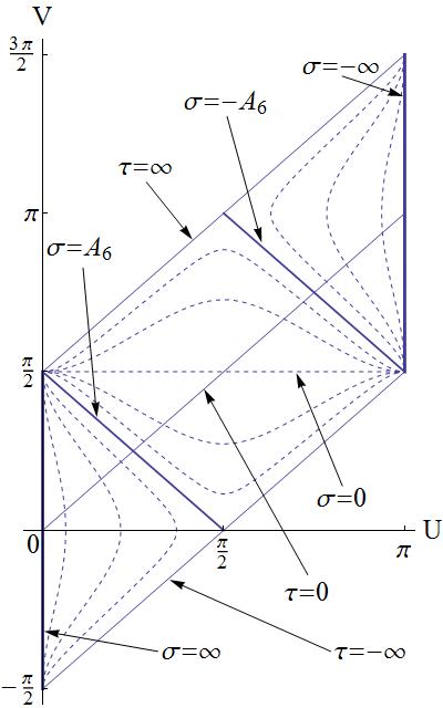
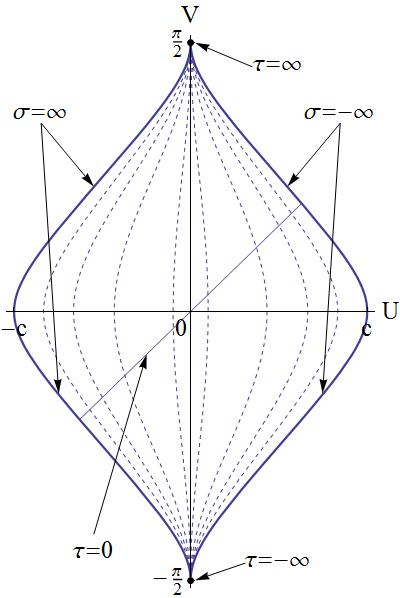
Figure 1: Penrose diagrams of the worldsheet for $A_{6}^{2}>0$ (left) and $A_{6}^{2}<0$ (right). Dashed lines are lines with constant $\sigma$. The two endpoints of the worldsheet correspond to the quark (at $\sigma=\infty$) and the antiquark (at $\sigma=-\infty$), which we depict with thick lines. In the second plot, they intersect the horizontal axis at $U=\pm c=\pm\arctan(\pi/2)$. Null trajectories going to the right correspond to constant $\tau$ in both plots.

Let us now consider the case with $A_{6}^{2}<0$. With the coordinate change

$$V=\frac{1}{2}\left(\arctan(\tau-\frac{2}{\sqrt{-A_{6}^{2}}}\arctan\,\frac{\sigma}{\sqrt{-A_{6}^{2}}})+\arctan\tau\right)$$ (3.7)

$$U=\frac{1}{2}\left(\arctan(\tau-\frac{2}{\sqrt{-A_{6}^{2}}}\arctan\,\frac{\sigma}{\sqrt{-A_{6}^{2}}})-\arctan\tau\right)$$ (3.8)

the metric can again be written as (3.6). The Penrose diagram for this case is also shown in figure 1 (right). There are no causal horizons and signals can go from the quark to the antiquark and vice-versa. This is just the Penrose diagram of $AdS_{2}$.

If we consider the string living in the Poincaré patch, only $A_{6}^{2}>0$ is possible. Moreover, the string is just defined for $\sigma\geq 0$ (there is no antiquark). Thus, one just has to keep the lower half of the plot on the left of figure 1. Of course, there is still a horizon at $\sigma=A_{6}$, no signal from $\sigma<A_{6}$ can reach the quark at $\sigma=\infty$.

Discussion

We have already mentioned that when the bulk is the Poincaré patch of $AdS$, the dual theory lives in a flat ${\rm I\kern-1.6pt{\rm R}}^{1,3}$ space. One can think of it as the decompactification limit of ${\rm I\kern-1.6pt{\rm R}}\times S^{3}$ when the radius of the sphere diverges $b\to\infty$. Comparing (3.2) to (2.35), we see that $A_{6}^{2}=A_{4}^{2}$ in this limit and therefore (3.5) tells us that the worldsheet temperature has to be associated to the proper acceleration of the quark. It seems that we are just recovering Unruh’s formula (1.1). However, the result is very surprising because (3.5) is valid for any stationary motion and not just for uniform acceleration. Thus, in this sense, the situation at strong coupling looks simpler. We will further comment on this fact in appendix A, but a deeper understanding of this phenomenon requires further work.

When the dual theory lives in ${\rm I\kern-1.6pt{\rm R}}\times S^{3}$, it is not true any more that the proper acceleration gives the worldsheet temperature since $A_{6}\neq A_{4}$. In fact, from (2.35), (2.30), (3.2) we find the interesting structure

$$A_{4}^{2}>{\cal P}_{q}>A_{6}^{2}\,\,,$$ (3.9)

In the decompactification limit $b\to\infty$, these three quantities coincide. Let us also consider the following relation

$$A_{6}^{2}=A_{4}^{2}-\frac{1+v^{2}}{(1-v^{2})b^{2}}\,\,.$$ (3.10)

Whenever $A_{6}^{2}<0$, there is no horizon and it does not make sense to define $T_{ws}$. From (3.10) we also see that it is possible to have non-zero proper acceleration $A_{4}$ and nevertheless the detector will remain inert. We shall provide an explicit example of this in section 4. Equation (3.10) is reminiscent of the results of [41, 42], where particles moving in $AdS$ where studied with the Unruh-De Witt formalism. The curvature of space-time may set a non-trivial lower bound on the proper acceleration necessary to start feeling effects of the quantum vacuum. See also [43] for recent progress in related subjects.

It is worth mentioning that (3.10) is a particular case of the general formula given in [44] relating the acceleration in a curved space to the acceleration in some ambient flat space which in our conventions reads $A_{6}^{2}=A_{4}^{2}+K_{uu}^{2}$ for $K_{uu}^{2}=-\eta_{MN}K_{uu}^{M}K_{uu}^{N}$ where

$$K_{uu}^{M}=U^{\alpha}U^{\beta}(\partial_{\alpha}\partial_{\beta}l^{M}-\Gamma_{\alpha\beta}^{\gamma}\partial_{\gamma}l^{M})\,\,.$$ (3.11)

4 Quarks rotating in circular paths

As advertised in the introduction, in this section we will study the problem of what happens to an accelerated observer undergoing circular motion in a bounded space. To address this question we will use the solution (2.24) restricted to a circular motion parallel to the equator but let us first review some early results for a quark rotating in 4d Minkowski space.

In [32] a quark rotating with constant angular velocity $\omega$ in Minkowski space was studied. The solution for the string found in that letter is a particular case of (2.9) as we showed in section 2.1. We wrote the embedding functions in (2.15).

A worldsheet horizon develops in the string worldsheet and it is located at $z_{h}=1/(\gamma^{2}\omega v)$ where $\gamma^{2}\omega v$ is the proper acceleration of the quark. From the perspective of an inertial observer, the quark emits gluonic radiation and this translates into stochastic fluctuation above the classical trajectory. From the point of view of the quark itself, we know that it does not see a thermal medium (i.e. there is no acceleration horizon), however, as explained in the introduction the detector clicks. This is of course consistent with the results of [6, 13]. The authors of [32] also calculated the total power radiated by the quark and found that, as for ordinary synchrotron radiation, it is proportional to the square of the proper acceleration of the 4d motion

$$P=\frac{\sqrt{\lambda}}{2\pi}A_{4}^{2}=\frac{\sqrt{\lambda}}{2\pi}\gamma^{4}\omega^{2}v^{2}\,\,,$$ (4.1)

in agreement with [31].

Quark rotating in a non-maximal circle of $S^{3}$

In order to pursue the ideas of [13] in a strong coupling situation, we want to consider rotation of a quark in a bounded space-time and check that the finiteness of space has a decisive influence on whether detectors click — namely on whether non-geodesic observers measure non-trivial excitations associated to fluctuations of the quantum vacuum. In the $AdS$/CFT framework, this is naturally implemented by analysing open strings living in global $AdS$, which are dual to quarks probing a theory which lives in ${\rm I\kern-1.6pt{\rm R}}\times S^{3}$.

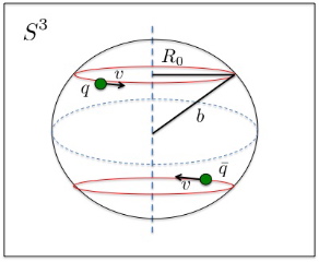
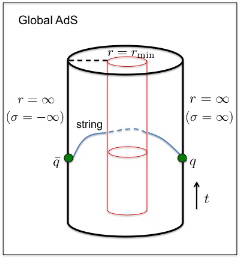
\begin{picture}(0.0,0.0)\end{picture}

Figure 2: Left: Schematic representation of the quark and antiquark rotating in the $S^{3}$. The latter is located at the antipode. Right: representation of global $AdS$. The quark/endpoint is located at the boundary $r=\infty$, the string goes into the bulk, reaches a minimum value $r=r_{\text{min}}$ and comes back to the boundary. The shape of the string is just a cartoon.

In section 2.2 we have written the general solution for a string moving in global $AdS$, see equation (2.24) and remember the radius of the $S^{3}$ was taken to one, $b=1$. We now want to consider the particular case in which the string endpoint is moving with constant angular velocity along a non-maximal circle of the $S^{3}$ (see Figure 2). The first step is to give an explicit representation of the $n^{a}$ defined in section 2.2 in terms of a set of coordinates parameterizing the $S^{3}$. We write

$$n^{1}=\sqrt{1-R^{2}}\,\,,\qquad\qquad\quad n^{2}=R\cos\theta\,\,,$$

$$n^{3}=R\sin\theta\cos\phi\,\,,\qquad n^{4}=R\sin\theta\sin\phi\,\,.$$ (4.2)

with $R\in[0,1]$, $\theta\in[0,\pi)$ and $\phi\in[0,2\pi)$. The metric of the unit $S^{3}$ then reads

$$d\Omega_{3}^{2}=\frac{dR^{2}}{1-R^{2}}+R^{2}d\theta^{2}+R^{2}\sin\theta d\phi^{2}\,\,.$$ (4.3)

Let us now consider the string endpoint to be in circular motion with constant velocity in the azimuthal angle $\phi$ (see Figure 2):

$$\bar{R}(\tau)=R_{0}\,\,,\qquad\bar{\phi}(\tau)=\omega\,t_{ret}(\tau)\,\,,\qquad\bar{\theta}(\tau)=\frac{\pi}{2}$$ (4.4)

where $R_{0}$ is the radius of the trajectory at the boundary. We can read the quantities defined in (2.21), (2.31):

$$v^{2}=R_{0}^{2}\omega^{2}\,\,,\qquad\vec{v}\cdot\vec{a}=0\,\,,\qquad a^{2}=R_{0}^{2}\omega^{4}\,\,.$$ (4.5)

From (2.20) we also know that

$${t_{\mbox{\scriptsize ret}}}=\frac{\tau}{\sqrt{1-\omega^{2}R^{2}_{0}}}=\gamma\tau\,\,.$$ (4.6)

Restricting (2.24) to this rotating quark ansatz, the string embedding is given by

$$t(\tau,\sigma) = \gamma\tau+\arctan\left(\frac{\gamma}{\sigma}\right)\,\,,$$

$$r(\tau,\sigma) = \sqrt{\sigma^{2}+\gamma^{2}\omega^{2}R^{2}_{0}}\,\,,$$

$$\theta(\tau,\sigma) = \frac{\pi}{2}\,\,,$$

$$\phi(\tau,\sigma) = \gamma\omega\tau+\arctan\left(\frac{\gamma\omega}{\sigma}\right)\,\,,$$

$$R(\tau,\sigma) = R_{0}\sqrt{\frac{\sigma^{2}+\gamma^{2}\omega^{2}}{\sigma^{2}+\gamma^{2}\omega^{2}R^{2}_{0}}}\,\,.$$ (4.7)

The solution written in this form is not very illuminating. We can eliminate the first two equations in (4) by rewriting the solution just as a function of $t$ and $r$. The result is

$$R(r)=R_{0}\sqrt{\frac{1+\gamma^{2}\omega^{2}}{r^{2}}(1-R^{2}_{0})}$$ (4.8)

and

$$\phi(t,r)=\omega t-\omega\arctan({\frac{\gamma}{\sqrt{1+r^{2}-\gamma^{2}}}})+\arctan({\frac{\omega\gamma}{\sqrt{1+r^{2}-\gamma^{2}}}})\,\,.$$ (4.9)

Reinserting the $S^{3}$ radius $b$ and taking the appropriate decompactification limit, it is not difficult to check that (4.8), (4.9) reduce to (2.15). As expected, when $\sigma\rightarrow\infty$ then $R(r)\rightarrow R_{0}$ and $\phi(t,r)\rightarrow\omega t$. Notice also that the embedding functions are not well defined for all values of the coordinate $r$. From (4.9) it is straightforward to see that $r\in(r_{\text{min}},\infty)$ where $r_{\text{min}}=\gamma\omega R_{0}$, which corresponds to $\sigma=0$ (see Figure 2).

Plugging (4.5) into (2.30), (2.35), (3.2), we can read the quantities:

$${\cal P}_{q}=\gamma^{4}R_{0}^{2}\omega^{2}(\omega^{2}-1)\,\,,\quad A_{4}^{2}=\gamma^{4}R_{0}^{2}\omega^{4}(1-R_{0}^{2})\,\,,\quad A_{6}^{2}=\gamma^{4}(R_{0}^{2}\omega^{4}-1)\,\,.$$ (4.10)

Let us now try to extract some physical information from this solution. First, from the induced metric we can obtain the position of the worldsheet horizon. The result is

$$r_{H}=\sqrt{\gamma^{4}R^{2}_{0}\omega^{2}(\omega^{2}-1)-1}\,\,.$$ (4.11)

We are now dealing with a quark (detector) rotating in a bounded space so we expect to make contact with the results of [13]. It is clear from (4.11) that not for every value of $\omega$ and $R_{0}$ the string worldsheet develops a horizon. One way to see this is to fix the value of $R_{0}$ (i.e. fix the “latitude” at which the string endpoint is moving) and from (4.11) find the critical value $\omega=\omega_{c}$ for which a horizon appears. This happens when $r_{H}=r_{min}$, leading to

$$\omega_{c}=\frac{1}{\sqrt{R_{0}}}\,\,.$$ (4.12)

This is the same condition as demanding $A_{6}^{2}=0$. Of course the endpoint cannot exceed the speed of light, then we can conclude that the observer will feel a non-trivial interaction with the quantum vacuum for a range of angular velocities:

$$\frac{1}{\sqrt{R_{0}}}<\omega<\frac{1}{R_{0}}$$ (4.13)

This is in qualitative agreement with what happens in the weakly coupled case analyzed by Davies et al. [13]

It is also interesting to look at the value of the rate of energy flowing down the string from the quark to the antiquark ${\cal P}_{q}$, see (4.10). It turns out that at $\omega=1$, this quantity changes sign. This is precisely the value of $\omega$ at which a co-rotating observer in the equator moves at the speed of light, although we do not know whether there is any physical reason for this coincidence. Thus, there are three different physical regimes. Reinserting $b$ (the radius of the $S^{3}$) they are:

• $0<\omega\,b<1$

  There is no worldsheet horizon. A co-rotating observer at the equator follows a time-like trajectory. Moreover, the quark is not loosing energy (${\cal P}_{q}<0$), but rather gaining energy from the gluonic fields whereas the anti-quark located at the antipode does emit energy. Below we will show that the external force acting on the quark is also negative, meaning that in order to have a stationary motion we need to pullback the quark instead of pushing on it. This makes it clear that in this situation, one should definitely not consider the quark and antiquark as independent objects, but one should rather think of the whole system as a kind collective motion. Both finite size and strong coupling seem to play a role in order to make this possible. The particular case $\omega\,b=1$ implies that ${\cal P}_{q}=0$ (and also the external force vanishes), then, the quark and antiquark rotate without any energy flow along the string.

• $1<\omega\,b<\frac{1}{\sqrt{R_{0}}}$

  A would-be co-rotating observer at the equator would now move faster than the local speed of light. The total power radiated ${\cal P}_{q}$ is positive (and also the external force). Nevertheless, there is not a worldsheet horizon and according to our proposal this means that the detector is not interacting with the quantum vacuum. As explained in the introduction, a similar situation is observed in [13].

• $\frac{1}{\sqrt{R_{0}}}<\omega\,b<\frac{1}{R_{0}}$

  The presence of the worldsheet horizon indicates, from the point of view of the inertial observer, that the quark will fluctuate around its classical trajectory (stochastic motion), meaning that the detector is interacting non-trivially with the vacuum. It should be interesting to describe the stochastic motion of the endpoint/quark following the ideas of [17, 18] but we leave that for future work. In this regime, the quark is emitting gluonic radiation which, as explained before, lives for a finite amount of time before it reaches the antiquark and is absorbed.

Let us make a heuristic argument in order to explain the transition between the second and third regimes. Let us think of the quark in a trajectory near the pole of the sphere such that it does not really probe the finiteness of the space. In the limit $b\to\infty$, $R_{0}\to 0$ with $b\,R_{0}$ fixed, the situation is essentially as if the quark was rotating in Minkowski space [32], see section 2.1. Only the third regime exists in this limit and there must be a worldsheet horizon. Synchrotron radiation is emitted and the length-scale controlling the actual size of a pulse is $\gamma^{-3}a^{-1}$ [32]. The idea is that when the size of this pulse is of the same order as the radius of the $S^{3}$, namely $\gamma^{-3}a^{-1}\sim b$, one cannot think any more of a quantum process in which a gluon emitted at a point and absorbed at the antipode. In a sense, the wavelength of the emitted “gluon” is as large as the $S^{3}$. At this point, the stochastic process of backreaction to the radiation emission ceases to exist. If we go to $\omega\,b\sim\frac{1}{\sqrt{R_{0}}}$, we would have $\gamma$ of order one and indeed $\gamma^{-3}a^{-1}\sim b$. This could give a qualitative understanding of the $\omega_{c}\sim 1/\sqrt{R_{0}}$ behaviour. In order to make this connection more rigorous, one should compute, along the lines of [32], the profile of radiation for the present situation.

Force and momentum

As a consistency check we can calculate the total power radiated by the rotating quark but applying the techniques used in [32]. The external force acting on the string endpoint is given by

$$\mathcal{F}_{\phi}=\frac{\sqrt{\lambda}}{2\pi}\Pi^{\sigma}_{\phi}|_{\sigma=\infty}=-\frac{\sqrt{\lambda}}{2\pi}\frac{\partial\mathcal{L}}{\partial\phi^{\prime}}$$ (4.14)

where ^′ means $\partial/\partial\sigma$. For this particular case

$$\frac{\sqrt{\lambda}}{2\pi}\Pi^{\sigma}_{\phi}|_{\sigma=\infty}=\frac{\sqrt{\lambda}}{2\pi}\Pi=\frac{\sqrt{\lambda}}{2\pi}\gamma^{4}R^{2}_{0}\omega(\omega^{2}-1)\,\,.$$ (4.15)

Finally, using the fact that energy is conserved on the string worldsheet we can write

$$\omega\,\mathcal{F}_{\phi}=\frac{\sqrt{\lambda}}{2\pi}\gamma^{4}R^{2}_{0}\omega^{2}(\omega^{2}-1)$$ (4.16)

which is exactly $\frac{\sqrt{\lambda}}{2\pi}{\cal P}_{q}$, with ${\cal P}_{q}$ given in (4.10). The result in the Poincaré patch (4.1) is recovered neglecting the 1 inside the bracket. For the anti-quark endpoint, one gets the same result with opposite sign.

APPENDICES

Appendix A Global embedding in Minkowski space

In section 3 we checked that, whenever $A_{6}^{2}$ is constant and positive, there is a worldsheet horizon and its temperature can be associated to what one could loosely call the Unruh temperature, see (3.5). This poses a puzzle. On the one hand, we would only expect uniformly accelerated motion to precisely produce thermal effects. But we have found that any stationary motion with the same constant modulus of the proper acceleration produces exactly the same induced metric on the worldsheet and therefore, it will yield the same pattern of stochastic motion — at least along the directions transverse to the classical trajectory, including excitations along the internal space. There is no difference between uniform acceleration and other stationary motions, from this point of view. However, this is not a prove that the quark is, in general, immersed in a thermal bath. In this appendix, we will make a computation that singles out uniform acceleration: we will check that only in that case, every bit of the string worldsheet is locally immersed in a thermal bath.

Let us start by considering the local temperature as seen from any bit of the string worldsheet, at some given $\sigma$. That is, we compute a temperature depending on $\sigma$, making use of Tolman’s law for the worldsheet metric (3.4)

$$\hat{T}_{ws}(\sigma)=\frac{T_{ws}}{\sqrt{g_{\tilde{\tau}\tilde{\tau}}}}=\frac{T_{ws}}{\sqrt{\sigma^{2}-A_{6}^{2}}}\,\,.$$ (A.1)

Here and in the following, we use hats for quantities referring to the string bit located at a given $\sigma$.

Before proceeding further, it is useful to introduce notation for the higher derivatives of the position. The relativistic jerk and snap defined in [46] are, for a particle living in $n$-dimensional Minkowski space time with proper time $\tau$, $n$-velocity $U^{\mu}$ and $n$-acceleration $A^{\mu}=\partial_{\tau}U^{\mu}$:

$$\Sigma^{\mu}=\frac{dA^{\mu}}{d\tau}+(A^{\nu}A_{\nu})U^{\mu}\,\,,\qquad\Xi^{\mu}=\frac{d\Sigma^{\mu}}{d\tau}+(\Sigma^{\nu}A_{\nu})U^{\mu}\,\,,$$ (A.2)

such that $U^{\nu}\Sigma_{\nu}=U^{\nu}\Xi_{\nu}=0$. A particle in uniform acceleration has vanishing relativistic jerk $\Sigma^{\mu}$ and snap $\Xi^{\mu}$.

We can now compute a different temperature for the same string bit: we consider the string bit itself as a particle and compute the temperature it feels due to its motion within the $AdS_{5}$ space. In order to do that, we follow ideas of [41, 42] and find out how it moves within the GEMS (global embedding in Minkowski space) of $AdS$. The GEMS of $AdS$ is simply given by the $X^{M}$ of (2.1) and therefore we already have the expression for the motion in the GEMS written in (2.3). All of the following computations follow from this solution.

The proper time corresponding to the string bit is

$$\hat{\tau}(\sigma)=\tau\sqrt{\sigma^{2}-A_{6}^{2}}$$ (A.3)

such that

$$\hat{U}^{M}(\sigma)=\frac{dX^{M}}{d\hat{\tau}}=\frac{A^{M}+\sigma U^{M}}{\sqrt{\sigma^{2}-A_{6}^{2}}}$$ (A.4)

where we have introduced

$$U^{M}=\partial_{\tau}l^{M}\,\,,\qquad A^{M}=\partial_{\tau}U^{M}\,\,.$$ (A.5)

These quantities without hat refer to the motion of the string endpoint within the 6d space spanned by the $l^{M}$. Remember that $U^{M}U_{M}=1$, $A^{M}A_{M}=-A_{6}^{2}$. Let us also define $-\Sigma^{M}\Sigma_{M}\equiv\varsigma^{2}\,\,,\ -\Xi^{M}\Xi_{M}\equiv\xi^{2}$. For simplicity, we assume that $A_{6}^{2}$, $\varsigma^{2}$, $\xi^{2}$ are all constant as is the case for circular motion. The acceleration of the string bit at position $\sigma$ is $\hat{A}^{M}(\sigma)=\frac{d\hat{U}^{M}}{d\hat{\tau}}$. It is straightforward to compute its modulus

$$\hat{A}^{2}(\sigma)=-\hat{A}^{M}\hat{A}_{M}=\frac{A_{6}^{2}}{\sigma^{2}-A_{6}^{2}}+\frac{\varsigma^{2}}{(\sigma^{2}-A_{6}^{2})^{2}}\,\,.$$ (A.6)

Notice that in the right hand side, $A_{6}^{2}$ and $\varsigma^{2}$ refer to quantities associated to the motion of the string endpoint. Imagine we define an Unruh-like “acceleration temperature” as $\hat{T}_{A}(\sigma)=\frac{\hat{A}}{2\pi}$. Then, comparing to (A.1), we find that the local worldsheet temperature coincides with the acceleration temperature only when the boundary jerk vanishes, namely for uniform acceleration (a case studied in [26]). This is suggesting that the nature of the worldsheet is only really thermal in that case, as one would expect on general grounds.

On the other hand, the quantity $\hat{T}_{A}(\sigma)$ can really be considered as a temperature only if the relativistic jerk is small for the corresponding string bit [44]. The appropriate dimensionless quantity to be used as a measure of how small the jerk is was defined in [44, 46]. We find

$$(\hat{\lambda}^{(1)})^{2}=\left|\frac{\hat{\Sigma}^{M}\hat{\Sigma}_{M}}{(\hat{A}^{N}\hat{A}_{N})^{2}}\right|^{2}=\frac{(\sigma^{2}-A_{6}^{2})(\xi^{2}+\sigma^{2}\varsigma^{2})+\varsigma^{4}}{(A_{6}^{2}(\sigma^{2}-A_{6}^{2})+\varsigma^{2})^{2}}\,\,.$$ (A.7)

If the jerk and snap of the boundary trajectory vanish $\varsigma^{2}=\xi^{2}=0$, this quantity is identically zero. Otherwise, and provided there is a horizon ($A_{6}^{2}>0$), then we have $(\lambda^{(1)})^{2}=1$ precisely at $\sigma^{2}=A_{6}^{2}$. Thus, unless the quark is uniformly acclerated, it is not possible to have a small jerk for the whole string. This seems to point out that the string only is really in a thermal bath when the quark undergoes uniform acceleration. This is only possible when the field theory is defined in ${\rm I\kern-1.6pt{\rm R}}^{1,3}$, and not in ${\rm I\kern-1.6pt{\rm R}}\times S^{3}$.

Appendix B A non-singular coordinate transformation

As explained in the introduction, there are at least three different ways to understand the detection of particles from the point of view of an accelerated observer and all of them are equivalent in the uniformly accelerated case. For more general motions this is no longer true.

In this appendix we give the explicit coordinate transformation that relates the inertial observer to the accelerated one (sitting on the quark). We show that the transformation is non-singular and therefore the determinant of the jacobian matrix $\mathcal{J}(r,t,\phi,R,\theta)$ is different from zero. Given the embedding fuctions (4.8) and (4.9), the coordinate transformation is

$$t^{\prime} = t\,\,,$$

$$r^{\prime} = r\,\,,$$

$$\theta^{\prime} = \theta\,\,,$$

$$\phi^{\prime} = \phi-\omega t+\omega\arctan({\frac{\gamma}{\sqrt{1+r^{2}-\gamma^{2}}}})-\arctan({\frac{\omega\gamma}{\sqrt{1+r^{2}-\gamma^{2}}}})\,\,,$$

$$R^{\prime} = R-\sqrt{\frac{\gamma^{2}\omega^{2}R^{2}_{0}}{r^{2}}(1-R^{2}_{0})+R^{2}_{0}}\,\,.$$ (B.1)

which is non-singular everywhere. Using (B) we can calculate de determinant of the jacobian matrix, the result is

$$\det[{\mathcal{J}(r,t,\phi,R,\theta)}]=1$$ (B.2)

reflecting the fact that the Bogolubov transformation is trivial [8] or equivalently, that there is not an acceleration horizon present in the transformed metric. This is very different for example to what happens when using the Rindler coordinate system to go from Minkowski to Rindler space-time for which the $\det[{\mathcal{J}}]=0$ precisely at the location of the acceleration horizon.

References

- [1] W. G. Unruh, “Notes on black hole evaporation,” Phys. Rev. D 14, 870 (1976).
- [2] L. C. B. Crispino, A. Higuchi and G. E. A. Matsas, “The Unruh effect and its applications,” Rev. Mod. Phys. 80, 787 (2008) [arXiv:0710.5373 [gr-qc]].
- [3] S. A. Fulling, “Nonuniqueness of canonical field quantization in Riemannian space-time,” Phys. Rev. D 7, 2850 (1973).
- [4] B. S. DeWitt, “Quantum gravity: The new synthesis”, in “General Relativity: An Einstein Centenary Survey” (S. W. Hawking and W. Israel, Eds.), Cambridge University Press, Cambridge, 1979.
- [5] N. D. Birrell and P. C. Davies, “Quantum Fields in Curved Space,” Cambridge University Press, Cambridge, 1982.
- [6] T. Padmanabhan, “Why Does An Accelerated Detector Click?,” Class. Quant. Grav. 2, 117 (1985).
- [7] L. Sriramkumar and T. Padmanabhan, “Probes of the vacuum structure of quantum fields in classical backgrounds,” Int. J. Mod. Phys. D 11, 1 (2002) [arXiv:gr-qc/9903054].
- [8] J. R. Letaw and J. D. Pfautsch, “The Quantized Scalar Field In Rotating Coordinates,” Phys. Rev. D 22, 1345 (1980).
- [9] J. S. Bell and J. M. Leinaas, “Electrons As Accelerated Thermometers,” Nucl. Phys. B 212, 131 (1983). J. S. Bell and J. M. Leinaas, “The Unruh effect and quantum fluctuations of electrons in storage rings,” Nucl. Phys. B 284, 488 (1987). W. G. Unruh, “Acceleration radiation for orbiting electrons,” Phys. Rept. 307, 163 (1998) [arXiv:hep-th/9804158].
- [10] E. T. Akhmedov and D. Singleton, “On the relation between Unruh and Sokolov-Ternov effects,” Int. J. Mod. Phys. A 22, 4797 (2007) [arXiv:hep-ph/0610391]. E. T. Akhmedov and D. Singleton, “On the physical meaning of the Unruh effect,” Pisma Zh. Eksp. Teor. Fiz. 86, 702 (2007) [arXiv:0705.2525 [hep-th]].
- [11] J. R. Letaw and J. D. Pfautsch, “The Quantized Scalar Field In The Stationary Coordinate Systems Of Flat Space-Time,” Phys. Rev. D 24, 1491 (1981).
- [12] J. I. Korsbakken and J. M. Leinaas, “The Fulling-Unruh effect in general stationary accelerated frames,” Phys. Rev. D 70, 084016 (2004) [arXiv:hep-th/0406080].
- [13] P. C. W. Davies, T. Dray and C. A. Manogue, “The Rotating Quantum Vacuum,” Phys. Rev. D 53, 4382 (1996) [arXiv:gr-qc/9601034].
- [14] J. M. Maldacena, “The large N limit of superconformal field theories and supergravity,” Adv. Theor. Math. Phys. 2, 231 (1998) [Int. J. Theor. Phys. 38, 1113 (1999)] [arXiv:hep-th/9711200].
- [15] J. M. Maldacena, “Wilson loops in large N field theories,” Phys. Rev. Lett. 80, 4859 (1998) [arXiv:hep-th/9803002].
- [16] K. Tuchin, “Synchrotron radiation by fast fermions in heavy-ion collisions,” Phys. Rev. C 82, 034904 (2010) [arXiv:1006.3051 [nucl-th]].
- [17] J. de Boer, V. E. Hubeny, M. Rangamani and M. Shigemori, “Brownian motion in AdS/CFT,” JHEP 0907, 094 (2009) [arXiv:0812.5112 [hep-th]].
- [18] D. T. Son and D. Teaney, “Thermal Noise and Stochastic Strings in AdS/CFT,” JHEP 0907, 021 (2009) [arXiv:0901.2338 [hep-th]].
- [19] E. Kiritsis, JHEP 9910, 010 (1999). [hep-th/9906206].
- [20] G. C. Giecold, E. Iancu and A. H. Mueller, “Stochastic trailing string and Langevin dynamics from AdS/CFT,” JHEP 0907, 033 (2009) [arXiv:0903.1840 [hep-th]].
- [21] J. Casalderrey-Solana, K. Y. Kim and D. Teaney, “Stochastic String Motion Above and Below the World Sheet Horizon,” JHEP 0912, 066 (2009) [arXiv:0908.1470 [hep-th]].
- [22] U. Gursoy, E. Kiritsis, L. Mazzanti, F. Nitti, “Langevin diffusion of heavy quarks in non-conformal holographic backgrounds,” JHEP 1012, 088 (2010). [arXiv:1006.3261 [hep-th]].
- [23] M. Chernicoff and A. Guijosa, “Acceleration, Energy Loss and Screening in Strongly-Coupled Gauge Theories,” JHEP 0806, 005 (2008) [arXiv:0803.3070 [hep-th]].
- [24] F. Dominguez, C. Marquet, A. H. Mueller, B. Wu and B. W. Xiao, “Comparing energy loss and -broadening in perturbative QCD with strong coupling SYM theory,” Nucl. Phys. A 811, 197 (2008) [arXiv:0803.3234 [nucl-th]].
- [25] B. W. Xiao, “On the exact solution of the accelerating string in space,” Phys. Lett. B 665, 173 (2008) [arXiv:0804.1343 [hep-th]].
- [26] A. Paredes, K. Peeters and M. Zamaklar, “Temperature versus acceleration: the Unruh effect for holographic models,” JHEP 0904, 015 (2009) [arXiv:0812.0981 [hep-th]].
- [27] T. Hirayama, P. W. Kao, S. Kawamoto and F. L. Lin, “Unruh Effect and Holography,” arXiv:1001.1289 [hep-th].
- [28] K. Ghoroku, M. Ishihara, K. Kubo and T. Taminato, “Accelerated Quark and Holography for Confining Gauge theory,” arXiv:1010.4396 [hep-th].
- [29] M. C. Batoni Abdalla, M. Botta Cantcheff, D. L. Nedel, “Strings in horizons, dissipation and a simple interpretation of the Hagedorn temperature,” Eur. Phys. J. C54, 311-317 (2008). [hep-th/0703064 [HEP-TH]].
- [30] E. Caceres, M. Chernicoff, A. Guijosa and J. F. Pedraza, “Quantum Fluctuations and the Unruh Effect in Strongly-Coupled Conformal Field Theories,” JHEP 1006, 078 (2010) [arXiv:1003.5332 [hep-th]].
- [31] A. Mikhailov, “Nonlinear waves in AdS/CFT correspondence,” arXiv:hep-th/0305196.
- [32] C. Athanasiou, P. M. Chesler, H. Liu, D. Nickel and K. Rajagopal, “Synchrotron radiation in strongly coupled conformal field theories,” Phys. Rev. D 81, 126001 (2010) [arXiv:1001.3880 [hep-th]].
- [33] M. Chernicoff, J. A. Garcia and A. Guijosa, “Generalized Lorentz-Dirac Equation for a Strongly-Coupled Gauge Theory,” Phys. Rev. Lett. 102, 241601 (2009) [arXiv:0903.2047 [hep-th]].
- [34] M. Chernicoff, J. A. Garcia and A. Guijosa, “A Tail of a Quark in N=4 SYM,” JHEP 0909, 080 (2009) [arXiv:0906.1592 [hep-th]].
- [35] S. J. Sin and I. Zahed, “Holography of radiation and jet quenching,” Phys. Lett. B 608, 265 (2005) [arXiv:hep-th/0407215].
- [36] D. Bak and S. J. Rey, “Holographic view of causality and locality via branes in AdS/CFT correspondence,” Nucl. Phys. B 572, 151 (2000) [arXiv:hep-th/9902101].
- [37] C. G. . Callan and A. Guijosa, “Undulating strings and gauge theory waves,” Nucl. Phys. B 565, 157 (2000) [arXiv:hep-th/9906153].
- [38] D. Villarroel, “Larmor Formula In Curved Spaces,” Phys. Rev. D 11, 2733 (1975).
- [39] S. R. Das, T. Nishioka and T. Takayanagi, “Probe Branes, Time-dependent Couplings and Thermalization in AdS/CFT,” JHEP 1007, 071 (2010) [arXiv:1005.3348 [hep-th]].
- [40] D. Kothawala and T. Padmanabhan, “Response of Unruh-DeWitt detector with time-dependent acceleration,” Phys. Lett. B 690, 201 (2010) [arXiv:0911.1017 [gr-qc]].
- [41] S. Deser and O. Levin, “Accelerated detectors and temperature in (anti) de Sitter spaces,” Class. Quant. Grav. 14, L163 (1997) [arXiv:gr-qc/9706018].
- [42] S. Deser and O. Levin, “Mapping Hawking into Unruh thermal properties,” Phys. Rev. D 59, 064004 (1999) [arXiv:hep-th/9809159].
- [43] D. Jennings, “On the response of a particle detector in Anti-de Sitter spacetime,” Class. Quant. Grav. 27, 205005 (2010) [arXiv:1008.2165 [gr-qc]].
- [44] J. G. Russo and P. K. Townsend, “Accelerating Branes and Brane Temperature,” Class. Quant. Grav. 25, 175017 (2008) [arXiv:0805.3488 [hep-th]].
- [45] V. E. Hubeny, “Relativistic Beaming in AdS/CFT,” arXiv:1011.1270 [hep-th].
- [46] J. G. Russo and P. K. Townsend, “Relativistic Kinematics and Stationary Motions,” J. Phys. A 42, 445402 (2009) [arXiv:0902.4243 [hep-th]].