Exponential Convergence to the Maxwell Distribution For Some Class of Boltzmann Equations

Institute for Theoretical Physics, ETH Zurich, CH-8093, Zürich, Switzerland

Abstract

We consider a class of nonlinear Boltzmann equations describing return to thermal equilibrium in a gas of colliding particles suspended in a thermal medium. We study solutions in the space $L^{1}(\Gamma^{(1)},d\lambda),$ where $\Gamma^{(1)}=\mathbb{R}^{3}\times\mathbb{T}^{3}$ is the one-particle phase space and $d\lambda=d^{3}vd^{3}x$ is the Liouville measure on $\Gamma^{(1)}.$ Special solutions of these equations, called “Maxwellians,” are spatially homogenous static Maxwell velocity distributions at the temperature of the medium. We prove that, for dilute gases, the solutions corresponding to smooth initial conditions in a weighted $L^{1}$-space converge to a Maxwellian in $L^{1}(\Gamma^{(1)},d\lambda),$ exponentially fast in time.

Contents

1. 1 Physics Background
2. 2 Explicit Form of the Equation and Main Theorem
3. 3 Reformulation of the Boltzmann Equation  (2.1)
4. 4 Local Well-Posedness of Equation  (2.1)
5. 5 Propagator Estimates
   1. 5.1 Proof of Proposition  5.2
   2. 5.2 Proof of Lemma  5.3
   3. 5.3 Proof of Inequality ( 5.14)
6. 6 Proof of the Main Theorem
   1. 6.1 Proof of Lemma  6.1
7. A Proof of Lemma  3.1
8. B Proof of Lemma  5.5
   1. B.1 Proof of Lemma  B.2
   2. B.2 Proof of Lemma  B.3
   3. B.3 Simplicity of the Eigenvalue $0$

1 Physics Background

In this paper we study the phenomenon of “return to equilibrium” for a gas of particles suspended in a thermal medium, in the limit where the range, $D$, of two-body forces between pairs of particles tends to $0$, while $\rho D^{2}$ is kept constant, with $\rho$ the density of the gas (Boltzmann-Grad limit). We assume that the one-particle phase space, $\Gamma^{(1)},$ is given by

$$\Gamma^{(1)}=\mathbb{R}^{3}\times\mathbb{T}^{3},$$ (1.1)

where $\mathbb{T}^{3}=\mathbb{R}^{3}/L\mathbb{Z}^{3}$, $L\not=0$, is configuration space (a three-dimensional, flat torus of diameter L), and $\mathbb{R}^{3}$ is velocity space. Boltzmann’s hypothesis of “molecular chaos” is the assumption that the $n-$ particle correlation functions describing the initial state of the gas at time $t=0$ are given by an $n-$fold product

$$\prod_{j=1}^{n}g_{0}(v_{j},x_{j}),\ (v_{j},x_{j})\in\Gamma^{(i)},\ j=1,\cdots,n,\ n=1,2,3,\cdots,$$

of a one-particle density, $g_{0}(v,x)$, on $\Gamma^{(1)}.$ One expects that, in the Boltzmann-Grad limit, molecular chaos propagates from the initial state to the state of the gas at an arbitrary later time, i.e., that the $n-$particle correlation functions at time $t>0$ are given by

$$\prod_{j=1}^{n}g_{t}(v_{j},x_{j})$$

where $g_{t}$ is the solution of a Boltzmann equation with initial condition given by $g_{t=0}=g_{0};$ (see  [20] for important results in this direction).

In this paper, we assume that every particle in the gas interacts with a memory-less thermal medium of temperature $T>0.$ Physically, this assumption is quite natural. It appears to us, however, that the corresponding mathematical problems have not received the attention they deserve. Assuming first that the gas consists of a single particle, we expect that the time evolution of its state in the van Hove limit, where the strength, $\lambda$, of the interaction of the particle with the medium tends to $0$, but time is scaled by a factor $\lambda^{-2}$, is given by a linear Boltzmann equation of the form

$$\partial_{t}g+v\cdot\nabla_{x}g=-Lg+G[g],$$ (1.2)

where

$$(Lg)(v,x):=\nu_{0}(v)g(v,x),$$ (1.3)

with $\nu_{0}(v)=\int_{\mathbb{R}^{3}}r_{0}(u,v)\ d^{3}u$, is a “loss term”, and

$$G[g](v,x):=\int_{\mathbb{R}^{3}}r_{0}(v,u)\ g(u,x)\ d^{3}u$$ (1.4)

is a “gain term”. The kernel $r_{0}(u,v)$ is assumed to obey “detailed balance”, i.e.,

$$r_{0}(u,v)=r_{0}(v,u)e^{\frac{\beta m}{2}(|v|^{2}-|u|^{2})},$$ (1.5)

where $\beta=(k_{B}T)^{-1}$ denotes the inverse temperature, $m$ is the particle mass, and $\frac{m}{2}|v|^{2}$ is the kinetic energy of a non-relativistic particle of mass $m$ and velocity $v.$

The equation $\partial_{t}g+v\cdot\nabla_{x}g=0$ describes an inertial motion of a particle with velocity $v$ distributed over $\mathbb{T}^{3}$ according to $g_{t}(v,x)$. The right hand side of Equation  (1.2) describes the effects on the motion of the particle of its interactions with a thermal medium at temperature $T>0,$ in the van Hove limit; (see, e.g.  [9, 13]). Next, we consider a gas of $N\simeq\rho L^{3}$ particles interacting with each other and with the medium. (Here $\rho$ is the density of the gas and $L^{3}$ the volume of $\mathbb{T}^{3}$). We assume that the medium has no memory (i.e., that it equilibrates arbitrarily rapidly after each interaction with a particle) and that the interactions between the particles in the gas are given by a two-body potential of short range (possibly induced by exchange of modes of the thermal medium). Let $\frac{d\sigma}{d\omega}$ denote the differential cross section for scattering between two particles in the given two-body potential. Let $u$ and $v$ be the velocities of two incoming particles and $u^{\prime}$, $v^{\prime}$ their outgoing velocities after an elastic collision process. By energy-momentum conservation,

$$u^{\prime}=u-[(u-v)\cdot\omega]\omega,\ v^{\prime}=v+[(u-v)\cdot\omega]\omega,$$ (1.6)

where $\omega$ is a unit vector. We define

$$Q(g,g)(v,x):=\int[g(v^{\prime},x)g(u^{\prime},x)-g(v,x)g(u,x)]\ |u-v|\frac{d\sigma}{d\omega}d^{2}\omega d^{3}u.$$ (1.7)

Then the Boltzmann equation for the time evolution of the one-particle density, $g_{t}(v,x)$, of a gas of $N$ interacting particles coupled to the thermal medium takes the following form:

$$\partial_{t}g(v,x)+v\cdot\nabla_{x}g(v,x)=-\nu_{0}(v)g(v,x)+\int_{\mathbb{R}^{3}}r_{0}(v,u)g(u,x)\ d^{3}u+\kappa Q(g,g)(v,x),$$ (1.8)

where $\nu_{0}$ is as in  (1.3) and $r_{0}$ as in  (1.5), $Q(g,g)$ is given by  (1.7), and $\kappa$ is the number of moles of the gas. We are interested in solutions, $g_{t}(v,x)$, of  (1.8) with the properties that $g_{t}(v,x)\geq 0$ and $\int_{\Gamma^{(1)}}g_{t}(v,x)\ d^{3}vd^{3}x=1.$

Under “reasonable” assumptions (to be specified below) on the kernel $r_{0}$ and the cross section $\frac{d\sigma}{d\omega}$ (as a function of $\omega$ and of $u,\ v$), a local existence- and uniqueness theorem for smooth solution of  (1.8) corresponding to smooth initial conditions $g_{t=0}(v,x)=g_{0}(v,x)\geq 0,$ with $\int_{\Gamma^{(1)}}g_{0}(v,x)\ d^{3}vd^{3}x=1,$ has been established; (see, e.g.,  [33, 21, 27]). As a consequence, one may show that, for all times $t>0$ at which $g_{t}$ is known to exist,

• $g_{t}(v,x)\geq 0$ whenever $g_{0}(v,x)\geq 0;$

• $\int_{\Gamma^{(1)}}g_{t}(v,x)\ d^{3}vd^{3}x=\int_{\Gamma^{(1)}}g_{0}(v,x)\ d^{3}vd^{3}x=1;$

• $g(v,x)=Ce^{-\frac{\beta m}{2}|v|^{2}}$ is a static (time-independent) solution of  (1.8), for a positive constant $C$. These static solutions are henceforth called “Maxwellians”.

The purpose of this paper is to prove asymptotic stability of Maxwellians. Our main result says that, under suitable decay- and smoothness assumptions on the initial condition $g_{0}(v,x)$, with $\int_{\Gamma^{(1)}}g_{0}(v,x)\ d^{3}vd^{3}x=1,$ and for sufficiently small values of the mole number, $\kappa$, of the gas, a global solution, $g(v,x),$ satisfying (A) and (B) exists and converges to the Maxwellian $Ce^{-\frac{\beta m}{2}|v|^{2}}$ (independent of $x$), with $C=L^{-3}(\frac{\beta m}{2\pi})^{\frac{3}{2}},$ exponentially fast in time. This result describes the phenomenon of “exponential return to equilibrium” in a gas of particles suspended in a thermal medium. The velocity distribution of the particles inherits the temperature of the thermal medium thanks to the “detailed balance condition”  (1.5). A precise formulation of our result is presented in Theorem  2.1, below.

In the literature, one finds many results on the asymptotic stability of Maxwellians for the Boltzmann equation with $r_{0}\equiv 0$ and $\kappa$ arbitrary. One circle of results concerns the spatially homogeneous case, where $g(v,x)$ is independent of the position $x$. This direction of research has been pioneered by T. Carleman in  [6]. Further results can be found in  [15, 5, 7, 14, 26]. Another circle of results concerns the Boltzmann equation on an exponentially weighted $L^{2}$ space; see, e.g.  [30, 18, 19, 16]. The advantage of working in such spaces is that spectral theory on Hilbert space can be used.

From the point of view of physics, however, the space $L^{1}(\Gamma^{(1)},d\lambda)$, where $d\lambda$ is the Liouville measure on $\Gamma^{(1)}$, is the natural choice for a study of the Boltzmann equation  (1.8), because the function $g_{t}(v,x)$ has the interpretation of a probability density on $\Gamma^{(1)}.$ In this context, the existence of weak global solutions has been established in  [12]. In  [11, 17], the asymptotic stability of Maxwellians, for general initial conditions, has been studied under the assumption that global smooth solutions exist. In the spatially homogeneous case, such results appear, e.g. in  [1, 31, 10, 3, 23, 32, 4, 26].

When the nonlinearity $Q$ in  (1.8) is absent, the equation is known as neutron transport equation. In certain settings, the spectrum of the propagator generated by the linear operator, on spaces $L^{p},\ 1\leq p\leq\infty$, has been studied in  [24, 25].

In this paper, we study the simpler problem of Boltzmann equations describing a gas of particles interacting with a thermal medium that tunes the temperature of the asymptotic Maxwell velocity distribution. The simplifications in our analysis, as compared to the usual Boltzmann equation without thermal medium, arise from the presence of the linear gain- and loss terms on the right hand sides of  (1.2) and  (1.8); (see  (1.3),  (1.4)). The behavior of solutions of  (1.2), for large times, is well understood. One may then view the nonlinearity, $\kappa Q(g,g)$, in  (1.8) as a perturbation. More precisely, we propose to linearize solutions of  (1.8) around the Maxwellian found by solving  (1.2), as time $t\rightarrow\infty.$ We must then study the properties of a certain linear operator $L$ defined in Equation  (3.2), below. An important step in our analysis consists in proving an appropriate decay estimate for the linear evolution given by $e^{-tL}(1-P_{0})$, where $P_{0}$ is the Riesz projection onto the eigenspace of $L$ corresponding to the eigenvalue $0$, which is spanned by the Maxwellian. What complicates this problem is that, for physically relevant choices of $r_{0}$ and cross sections $\frac{d\sigma}{d\omega}$, the spectrum of the operator $L$ occupies the entire right half of the complex plane, except for a strip of strictly positive width around the imaginary axis that only contains the eigenvalue $0$; see Figure  5.1, below. Rewriting $e^{-tL}(1-P_{0})$ in terms of the resolvent, $(L-z)^{-1},$ of $L$,

$$e^{-tL}(1-P_{0})=-\frac{1}{2\pi i}\oint_{\Gamma}e^{-tz}(L-z)^{-1}\ dz,$$ (1.9)

(see, e.g.,  [28]), where the integration contour $\Gamma$ encircles the spectrum of $L$, except for the eigenvalue $0$, we encounter the problem of proving strong convergence of the integral on the right hand side of  (1.9) on $L^{1}$. This problem is solved in Section  5. We expect that an extension of our techniques can be used to prove a conjecture in  [29] concerning the exponential convergence of solutions of the Boltzmann equation to a Maxwell distribution. For the results in this direction, see [17] for a constructive proof, and [2] for a non-constructive proof.

Our paper is organized as follows. The main hypothesis on the kernel $r_{0}(u,v)$ and the cross section $\frac{d\sigma}{d\omega}$ and the main result, Theorem  2.1, of our analysis are described in Section  2. In Section  3, the Boltzmann equation  (1.8) is rewritten in a more convenient form; see Equation  (3.2). The local wellposedness of Equation  (3.2) is proven in Section  4. In Section  5, a decay estimate on the propagator, $e^{-tL}(1-P_{0})$, is established. This represents the technically most demanding part of our analysis. The proof of our main result is completed in Section  6. Three appendices contain some technical details.

2 Explicit Form of the Equation and Main Theorem

We use the notation $g_{t}(v,x)=:g(v,x,t)$, $(v,x)\in\mathbb{R}^{3}\times\mathbb{T}^{3},$ $t\in\mathbb{R},$ and consider the equation (see  (1.8))

$$\partial_{t}g+v\cdot\nabla_{x}g=-\nu_{0}g+\int_{\mathbb{R}^{3}}r_{0}(v,u)g(u,\cdot)\ d^{3}u+\kappa Q(g,g)$$ (2.1)

with initial condition

$$g(v,x,0)=g_{0}(v,x)\geq 0,\ \ x\in\mathbb{R}^{3}/(2\pi\mathbb{Z})^{3}\ (\text{i.e.,}\ L=2\pi).$$

The different terms on the right hand side are chosen as follows.

• The function $\nu_{0}:\mathbb{R}^{3}\rightarrow\mathbb{R}^{+}$ is defined by

  $$\nu_{0}(v):=\int_{\mathbb{R}^{3}}r_{0}(u,v)\ d^{3}u.$$ (2.2)

• The function $r_{0}:\mathbb{R}^{3}\times\mathbb{R}^{3}\rightarrow\mathbb{R}^{+}$ must satisfy the detailed balance condition  (1.5). In the following, we set $\beta m=2.$ The example we have in mind is given by

  $$r_{0}(u,v):=e^{-|u|^{2}}(1+|u-v|^{2})^{\frac{1}{2}}.$$ (2.3)

  More generally, we require the following conditions on $r_{0}$: (a) There exists a positive constant $C>0$ such that

  $$\frac{1}{C}e^{-|u|^{2}}(1+|u-v|^{2})^{\frac{1}{2}}\leq r_{0}(u,v)\leq Ce^{-|u|^{2}}(1+|u-v|^{2})^{\frac{1}{2}}.$$

  (b) There exists a constant $C_{2}>0$ such that the derivatives of $r_{0}$ satisfies the condition

  $$|\partial_{u}^{k}\partial_{v}^{l}r_{0}(u,v)|\leq C_{2}e^{-\frac{1}{2}|u|^{2}}(1+|u-v|^{2})^{\frac{1-l}{2}}$$

  for $k+l\leq 1.$

• The constant $\kappa$ is positive and small.

• The nonlinearity $Q(g,g)$ is chosen to correspond to a hard-sphere potential:

  $$Q(g,g)(v,x):=\int_{\mathbb{R}^{3}\times\mathbb{S}^{2}}|(u-v)\cdot\omega|[g(u^{\prime},x)g(v^{\prime},x)-g(u,x)g(v,x)]\ d^{3}u\ d^{2}\omega,$$ (2.4)

  where $u^{\prime},v^{\prime}\in\mathbb{R}^{3}$ are given by $u^{\prime}:=u-[(u-v)\cdot\omega]\omega,$ $v^{\prime}:=v+[(u-v)\cdot\omega]\omega$, see Equations  (1.6),  (1.7).

We define a function $M:\mathbb{R}^{3}\rightarrow\mathbb{R}^{+}$ by

$$M(v):=e^{-|v|^{2}},$$

and a constant $C_{\infty}$ by

$$C_{\infty}:=\frac{\int_{\mathbb{R}^{3}\times\mathbb{T}^{3}}g_{0}(v,x)\ d^{3}vd^{3}x}{(2\pi)^{3}\int_{\mathbb{R}^{3}}M(v)\ d^{3}v}$$

and we set $\langle v\rangle:=\sqrt{1+|v|^{2}}.$

The main result of this paper is the following theorem:

Theorem 2.1.

We assume that

$$\sum_{|\alpha|\leq 8}\|\langle v\rangle^{m}\partial_{x}^{\alpha}g_{0}\|_{L^{1}(\mathbb{R}^{3}\times\mathbb{T}^{3})}\leq C$$

for a constant $C<\infty$ and for some sufficiently large $m>0,$ and that the constant $\kappa>0$ in  (2.1) is sufficiently small. Then there exist positive constants $C_{0}$, $C_{1}$ such that

$$\|g(\cdot,t)-C_{\infty}M\|_{L^{1}(\mathbb{R}^{3}\times\mathbb{T}^{3})}\leq C_{1}e^{-C_{0}t}.$$ (2.5)

This theorem will be proven in Section  6.

Concerning the choices of $r_{0}$ and the collision term $Q$ in  (2.1), we make the following remarks.

• We expect that our results hold under more general assumptions. For example, if $r_{0}(u,v)=e^{-|u|^{2}}h(|u-v|),$ where $h$ is a strictly positive, smooth bounded function, and if the collision term $|u-v|\frac{d\sigma}{d\omega}$ (see  (1.7)), is bounded then it becomes quite easy to prove a result similar to Theorem  2.1.

• If the collision term is unbounded then it simplifies life to impose the condition that $r_{0}$ is unbounded too. For technical details we refer to Equations  (4.10) and  (6.9) and the remarks thereafter.

• In our spectral analysis of the linear operator $L$, to be defined in  (3.3) below, the unboundedness of $\nu_{0}$ in  (2.1), which is defined in terms of $r_{0},$ is used. We believe that this is not essential, although it makes proofs simpler. In fact, by results proven in  [1, 26], one can generalize our results in Lemma  5.3.

3 Reformulation of the Boltzmann Equation  (2.1)

To facilitate later analysis we reformulate equation  (2.1) in a more convenient form. We define a function $f:\ \mathbb{R}^{3}\times\mathbb{T}^{3}\times\mathbb{R}^{+}\rightarrow\mathbb{R}$ by

$$f(v,x,t):=g(v,x,t)-C_{\infty}M(v),$$ (3.1)

with the constant $C_{\infty}$ and function $M$ defined before Theorem  2.1. From  (2.1) we derive an equation for $f,$

$$\partial_{t}f=-Lf+\kappa Q(f,f).$$ (3.2)

Here the nonlinear term $Q(f,f)$ is defined in  (2.4), the linear operator $L$ is defined by

$$L:=v\cdot\nabla_{x}+L_{0}+C_{\infty}\kappa L_{1}.$$ (3.3)

Here $L_{0}$ and $L_{1}$ are defines as

• $$L_{0}:=\nu_{0}-K_{0},$$

  where $\nu_{0}$ is defined in  (2.2), and for any function $f$, $K_{0}$ is defined as

  $$K_{0}(f)(v):=\int_{\mathbb{R}^{3}}r_{0}(v,u)f(u)\ d^{3}u.$$ (3.4)

• $$L_{1}f:=\nu_{1}(v)f+K_{1}(f)$$ (3.5)

  where $\nu_{1}$ is the multiplication operator defined by

  $$\nu_{1}(v):=\int_{\mathbb{R}^{3}\times\mathbb{S}^{2}}|(u-v)\cdot\omega|M(u)\ d^{3}ud^{2}\omega,$$

  and $K_{1}(f)$ is given by

  $$\begin{array}[]{lll}K_{1}(f)&:=&2\pi\int_{\mathbb{R}^{3}}|u-v|^{-1}e^{-\frac{|(u-v)\cdot v|^{2}}{|u-v|^{2}}}f(u)\ d^{3}u-\pi\int_{\mathbb{R}^{3}}|u-v|e^{-|v|^{2}}f(u)\ d^{3}u\\ &&\\ &=&\int_{\mathbb{R}^{3}\times\mathbb{S}^{2}}|(u-v)\cdot\omega|M(u)f(u)\ d^{3}ud^{2}\omega\\ &&\\ &&-\int_{\mathbb{R}^{3}\times\mathbb{S}^{2}}|(u-v)\cdot\omega|M(u^{\prime})f(v^{\prime})\ d^{3}ud^{2}\omega\\ &&\\ &&-\int_{\mathbb{R}^{3}\times\mathbb{S}^{2}}|(u-v)\cdot\omega|M(v^{\prime})f(u^{\prime})\ d^{3}ud^{2}\omega\end{array}$$ (3.6)

  The explicit form of $K_{1}$ has been derived by R.T.Glassey in  [14], (see also  [15, 8]).

To simplify our notations, we define operators $K$ and $\nu$ by

$$K:=-K_{0}+C_{\infty}\kappa K_{1}$$ (3.7)

$$\nu:=\nu_{0}+C_{\infty}\kappa\nu_{1}.$$ (3.8)

Then the linear operator $L$ in  (3.2) is given by

$$L=\nu+v\cdot\nabla_{x}+K.$$

To prepare the ground for our analysis, we state some estimates on the nonlinearity $Q$ and the operators $\nu,$ $K_{0}$ and $K_{1}$. These estimates show that all these operators are unbounded.

Lemma 3.1.

There exists a positive constant $\Lambda$ such that

$$\nu_{0}(v),\ \nu_{1}(v)\geq\Lambda(1+|v|).$$ (3.9)

For any $m\geq 0,$ there exists a constant $C_{m}$ such that, for arbitrary functions $f,\ g\in L^{1}(\mathbb{R}^{3}),$

$$\|\langle v\rangle^{m}K_{0}f\|_{L^{1}(\mathbb{R}^{3})}\leq C_{m}\|\langle v\rangle f\|_{L^{1}(\mathbb{R}^{3})},$$ (3.10)

$$\|\langle v\rangle^{m}K_{1}f\|_{L^{1}(\mathbb{R}^{3})}\leq C_{m}\|\langle v\rangle^{m+1}f\|_{L^{1}(\mathbb{R}^{3})},$$ (3.11)

and

$$\begin{array}[]{lll}\|\langle v\rangle^{m}Q(f,g)\|_{L^{1}(\mathbb{R}^{3})}&\leq&C_{m}\|f\|_{L^{1}(\mathbb{R}^{3})}\|\langle v\rangle^{m+1}g\|_{L^{1}(\mathbb{R}^{3})}+C_{m}\|\langle v\rangle^{m+1}f\|_{L^{1}(\mathbb{R}^{3})}\|g\|_{L^{1}(\mathbb{R}^{3})}.\end{array}$$ (3.12)

This lemma is proven in Appendix  A.

4 Local Well-Posedness of Equation  (2.1)

In this section we prove local wellposedness of equation  (2.1).

We briefly present the ideas used in the proof. One of the difficulties tackled in the present paper is that the nonlinearity $Q(f,f)$ is unbounded; see  (3.12). To overcome it we adopt a technique drawn from the works  [18, 19]. Specifically, we consider the solution $f$ in a Banach space to be defined in  (4.2) below, the second term in its definition playing a crucial role in controlling $Q(f,f)$. For computational details we refer to  (4.10) below.

The main result of this section is

Proposition 4.1.

If the constant $\kappa>0$ in  (2.1) is sufficiently small and if

$$\sum_{|\alpha|\leq 8}\|\langle v\rangle^{m}\partial_{x}^{\alpha}f_{0}\|_{L^{1}(\mathbb{R}^{3}\times\mathbb{T}^{3})}\leq\kappa^{-\frac{1}{4}},$$

for some $m\geq 2,$ then there exists a constant $T=T(\kappa)$ such that, on the interval $[0,T],$ equation  (3.2) has a unique solution $f$ satisfying

$$\sum_{|\alpha|\leq 8}\|\langle v\rangle^{m}\partial_{x}^{\alpha}f(\cdot,t)\|_{L^{1}(\mathbb{R}^{3}\times\mathbb{T}^{3})}+\int_{0}^{t}\|\langle v\rangle^{m+1}\partial_{x}^{\alpha}f(\cdot,s)\|_{L^{1}(\mathbb{R}^{3}\times\mathbb{T}^{3})}\ ds\leq\kappa^{-\frac{1}{2}}.$$

Proof.

To simplify the notation we denote $L^{1}(\mathbb{R}^{3}\times\mathbb{T}^{3})$ by $L^{1}$.

To recast  (3.2) in a convenient form, we rewrite this equation using Duhamel’s principle,

$$f(t)=e^{-t[\nu+v\cdot\nabla_{x}]}f_{0}+\int_{0}^{t}e^{-(t-s)(\nu+v\cdot\nabla_{x})}H(f(s))\ ds,$$ (4.1)

with $H(f):=-K_{0}f+C_{\infty}\kappa K_{1}f+\kappa Q(f,f)$.

In order to be able to apply suitable results of functional analysis, we demand that $f$ and the terms on the right hand side belong to a suitable Banach space. We define a family of Banach spaces, $\mathcal{B}_{\delta}$, $0<\delta\ll 1,$ by

$$\mathcal{B}_{\delta}:=\{g:\mathbb{R}^{3}\times\mathbb{T}^{3}\times[0,\delta]\rightarrow\mathbb{C}|\ \|g\|_{\mathcal{B}_{\delta}}<\infty\}$$

where $\|g\|_{\mathcal{B}_{\delta}}$ is defined by

$$\|g\|_{\mathcal{B}_{\delta}}:=\sum_{|\alpha|\leq 8}[\sup_{0\leq s\leq\delta}\|\langle v\rangle^{m}\partial_{x}^{\alpha}g(\cdot,s)\|_{L^{1}}+\int_{0}^{\delta}\|\langle v\rangle^{m+1}\partial_{x}^{\alpha}g(\cdot,s)\|_{L^{1}}\ ds].$$ (4.2)

Our key observations are:

• $$\|e^{-t[\nu+v\cdot\nabla_{x}]}f_{0}\|_{\mathcal{B}_{\delta}}\leq\displaystyle\sum_{|\alpha|\leq 8}\|\langle v\rangle^{m}\partial_{x}^{\alpha}f_{0}\|_{L^{1}};$$ (4.3)

• We define a nonlinear map, $\Pi,$ by

  $$\Pi(f,t):=\int_{0}^{t}e^{-(t-s)(\nu+v\cdot\nabla_{x})}H(f(s))\ ds.$$

  Then $\Pi:\ \mathcal{B}_{\delta}\rightarrow\mathcal{B}_{\delta}$ is a contractive map if restricted to a suitable domain. More specifically,

  $$\|\Pi(f)-\Pi(g)\|_{\mathcal{B}_{\delta}}\leq\frac{1}{2}\|f-g\|_{\mathcal{B}_{\delta}},$$ (4.4)

  provided $\|f\|_{\mathcal{B}_{\delta}},\ \|g\|_{\mathcal{B}_{\delta}}\leq\kappa^{-\frac{1}{4}},$ and for $\delta$ sufficiently small.

Obviously these two results,  (4.3) and  (4.4), together with the contraction lemma, imply the existence of a unique solution in the time interval $[0,\delta],$ provided that $\delta=\delta(\kappa)$ is sufficiently small.

In what follows we prove  (4.3) and  (4.4).

To prove  (4.4), we start by estimating $\|\langle v\rangle^{m}\partial_{x}^{\alpha}[\Pi(f)-\Pi(g)]\|_{L^{1}},\ |\alpha|\leq 8.$ We decompose this quantity into three terms:

$$\begin{array}[]{lll}&&\|\langle v\rangle^{m}\int_{0}^{t}e^{-(t-s)(\nu+v\cdot\nabla_{x})}\partial_{x}^{\alpha}[H(f(s))-H(g(s))]\ ds\|_{L^{1}}\\ &&\\ &\leq&\int_{0}^{t}\|\langle v\rangle^{m}e^{-(t-s)(\nu+v\cdot\nabla_{x})}\partial_{x}^{\alpha}[H(f(s))-H(g(s))]\|_{L^{1}}ds\\ &&\\ &\leq&\int_{0}^{t}\|\langle v\rangle^{m}\partial_{x}^{\alpha}[H(f(s))-H(g(s))]\|_{L^{1}}ds\\ &&\\ &\lesssim&\int_{0}^{t}\|\langle v\rangle^{m}\partial_{x}^{\alpha}K_{0}(f(s)-g(s))\|_{L^{1}}\ ds+\kappa C_{\infty}\int_{0}^{t}\|\langle v\rangle^{m}K_{1}\partial_{x}^{\alpha}(f(s)-g(s))\|_{L^{1}}\ ds\\ &&\\ &&+\kappa\int_{0}^{t}\|\langle v\rangle^{m}\partial_{x}^{\alpha}[Q(f,f)(s)-Q(g,g)(s)]\ \|_{L^{1}}\ ds\\ &&\\ &=&\Psi_{1}+\Psi_{2}+\Psi_{3},\end{array}$$ (4.5)

where in the third step we use the fact that the operator $e^{tv\cdot\nabla_{x}}$ preserves $L^{1}$ norm. The terms $\Psi_{k},\ k=1,2,3,$ are defined in the obvious manner and are estimated below.

1. By Lemma  3.1, inequality  (3.10),

   $$\begin{array}[]{lll}\Psi_{1}&=&\int_{0}^{t}\|\langle v\rangle^{m}K_{0}\partial_{x}^{\alpha}(f(s)-g(s))\|_{L^{1}}\ ds\\ &&\\ &\lesssim&\int_{0}^{t}\|\langle v\rangle\partial_{x}^{\alpha}(f-g)\|_{L^{1}}\ ds\\ &&\\ &\leq&t\|f-g\|_{\mathcal{B}_{\delta}},\ \text{for}\ t\leq\delta.\end{array}$$ (4.6)

2. From Lemma  3.1, inequality  (3.11) we deduce that

   $$\Psi_{2}\lesssim\kappa C_{\infty}\int_{0}^{t}\|\langle v\rangle^{m+1}\partial_{x}^{\alpha}(f(s)-g(s))\|_{L^{1}}\ ds\lesssim\kappa C_{\infty}\|f-g\|_{\mathcal{B}_{\delta}},$$ (4.7)

   for $t\leq\delta$.

3. To estimate $\Psi_{3},$ we use the definition of $Q$ to obtain

   $$\Psi_{3}\leq\kappa\int_{0}^{t}\|\langle v\rangle^{m}\partial_{x}^{\alpha}Q(f-g,f)(s)\|_{L^{1}}+\|\langle v\rangle^{m}\partial_{x}^{\alpha}Q(g,f-g)(s)\|_{L^{1}}\ ds.$$

   Using  (4.13), below, we find that

   $$\begin{array}[]{lll}\Psi_{3}&\leq&\displaystyle\kappa\int_{0}^{t}\{\sum_{|\beta_{1}|\leq 8}\|\langle v\rangle^{m+1}\partial_{x}^{\beta_{1}}(f-g)\|_{L^{1}}\sum_{|\beta_{2}|\leq 8}(\|\partial_{x}^{\beta_{2}}f\|_{L^{1}}+\|\partial_{x}^{\beta_{2}}g\|_{L^{1}})\ \}ds\\ &&\\ &&+\kappa\displaystyle\int_{0}^{t}\{\sum_{|\beta_{1}|\leq 8}\|\partial_{x}^{\beta_{1}}(f-g)\|_{L^{1}}\sum_{|\beta_{2}|\leq 8}(\|\langle v\rangle^{m+1}\partial_{x}^{\beta_{2}}f\|_{L^{1}}+\|\langle v\rangle^{m+1}\partial_{x}^{\beta_{2}}g\|_{L^{1}})\ \}ds\\ &&\\ &\lesssim&\kappa\|f-g\|_{\mathcal{B}_{\delta}}[\|f\|_{\mathcal{B}_{\delta}}+\|g\|_{\mathcal{B}_{\delta}}].\end{array}$$ (4.8)

Collecting these estimates, we conclude, that for any $t\leq\delta\ll 1,$

$$\|\langle v\rangle^{m}\partial_{x}^{\alpha}[\Pi(f)-\Pi(g)]\|_{L^{1}}\lesssim\|f-g\|_{\mathcal{B}_{\delta}}[C_{\infty}\kappa+\kappa(\|f\|_{\mathcal{B}_{\delta}}+\|g\|_{\mathcal{B}_{\delta}})+\delta].$$ (4.9)

Next, we estimate $\int_{0}^{t}\|\langle v\rangle^{m+1}\partial_{x}^{\alpha}[\Pi(f(s))-\Pi(g(s))]\|_{L^{1}}\ ds$. By direct computation,

$$\begin{array}[]{lll}&&\int_{0}^{t}\|\int_{0}^{s}e^{-(s-s_{1})(\nu+v\cdot\nabla_{x})}\langle v\rangle^{m+1}\partial_{x}^{\alpha}[H(f(s_{1}))-H(g(s_{1}))]\ ds_{1}\|_{L^{1}}\ ds\\ &&\\ &\leq&\int_{0}^{t}\int_{0}^{s}\|e^{-(s-s_{1})(\nu+v\cdot\nabla_{x})}\langle v\rangle^{m+1}\partial_{x}^{\alpha}[H(f(s_{1}))-H(g(s_{1}))]\|_{L^{1}}\ ds_{1}ds\\ &&\\ &=&\int_{0}^{t}\int_{0}^{s}\|e^{-(s-s_{1})\nu}\langle v\rangle^{m+1}\partial_{x}^{\alpha}[H(f(s_{1}))-H(g(s_{1}))]\|_{L^{1}}\ ds_{1}ds\\ &&\\ &=&\|\int_{0}^{t}\int_{0}^{s}e^{-(s-s_{1})\nu}|\langle v\rangle^{m+1}\partial_{x}^{\alpha}[H(f(s_{1}))-H(g(s_{1}))]|\ ds_{1}ds\|_{L^{1}}\\ &&\\ &\leq&\|\int_{0}^{t}\nu^{-1}\langle v\rangle^{m+1}|\partial_{x}^{\alpha}[H(f(s))-H(g(s))]|\ ds\|_{L^{1}}\\ &&\\ &\lesssim&\int_{0}^{t}\|\langle v\rangle^{m}\partial_{x}^{\alpha}[H(f(s))-H(g(s))]\|_{L^{1}}ds,\end{array}$$ (4.10)

where the crucial step is the fourth one and is accomplished by integrating by parts in the variable $s,$ the last inequality results from our estimate on $\nu=\nu_{0}+C_{\infty}\kappa\nu_{1}$ in  (3.9). Here the condition on $r_{0}$ being unbounded, (see  (2.2)), is used.

We observe that the last step in  (4.10) is the same to that in the third line of  (4.5). Hence it also admits the estimate in  (4.9), i.e.,

$$\int_{0}^{t}\|\langle v\rangle^{m+1}\partial_{x}^{\alpha}[\Pi(f(s))-\Pi(g(s))]\|_{L^{1}}\ ds\lesssim\|f-g\|_{\mathcal{B}_{\delta}}[C_{\infty}\kappa+\delta+\kappa(\|f\|_{\mathcal{B}_{\delta}}+\|g\|_{\mathcal{B}_{\delta}})].$$ (4.11)

This, together with  (4.9), implies  (4.4).

Next, we prove  (4.3). By direct computation

$$\begin{array}[]{lll}\|e^{-t[\nu+v\cdot\nabla_{x}]}f_{0}\|_{\mathcal{B}_{\delta}}&=&\displaystyle\sum_{|\alpha|\leq 8}[\displaystyle\sup_{0\leq t\leq\delta}\|\langle v\rangle^{m}e^{-t[\nu+v\cdot\nabla_{x}]}\partial_{x}^{\alpha}f_{0}\|_{L^{1}}+\int_{0}^{t}\|\langle v\rangle^{m+1}e^{-s(\nu+v\cdot\nabla_{x})}\partial_{x}^{\alpha}f_{0}\|_{L^{1}}\ ds]\\ &&\\ &=&\displaystyle\sum_{|\alpha|\leq 8}[\|\langle v\rangle^{m}\partial_{x}^{\alpha}f_{0}\|_{L^{1}}+\|\int_{0}^{t}e^{-s\nu}\ ds\ \langle v\rangle^{m+1}|\partial_{x}^{\alpha}f_{0}|\|_{L^{1}}]\\ &&\\ &\leq&\displaystyle\sum_{|\alpha|\leq 8}\|\langle v\rangle^{m}\partial_{x}^{\alpha}f_{0}\|_{L^{1}}\end{array}$$

which is  (4.3). ∎

In the proof we have used the following embedding results; (see  (4.8)).

Lemma 4.2.

For any function $f:\ \mathbb{R}^{3}\times\mathbb{T}^{3}\rightarrow\mathbb{C},$

$$\sup_{x\in\mathbb{Z}^{3}}\|f(\cdot,x)\|_{L^{1}(\mathbb{R}^{3})}\leq C\sum_{|\alpha|\leq 4}\|\partial_{x}^{\alpha}f\|_{L^{1}(\mathbb{R}^{3}\times\mathbb{T}^{3})}.$$ (4.12)

For any $\alpha\in(\mathbb{Z}^{+})^{3}$ satisfying $|\alpha|\leq 8$, and for arbitrary functions $f,\ g:\ \mathbb{R}^{3}\times\mathbb{T}^{3}\rightarrow\mathbb{C},$

$$\begin{array}[]{lll}\|\langle v\rangle^{m}\partial_{x}^{\alpha}Q(f,g)\|_{L^{1}(\mathbb{R}^{3}\times\mathbb{T}^{3})}&\lesssim&\displaystyle\sum_{|\beta_{1}|,\ |\beta_{2}|\leq 8}[\|\langle v\rangle^{m+1}\partial_{x}^{\beta_{1}}f\|_{L^{1}(\mathbb{R}^{3}\times\mathbb{T}^{3})}\|\partial_{x}^{\beta_{2}}g\|_{L^{1}(\mathbb{R}^{3}\times\mathbb{T}^{3})}\\ &&\\ &+&\|\langle v\rangle^{m+1}\partial_{x}^{\beta_{1}}g\|_{L^{1}(\mathbb{R}^{3}\times\mathbb{T}^{3})}\|\partial_{x}^{\beta_{2}}f\|_{L^{1}(\mathbb{R}^{3}\times\mathbb{T}^{3})}].\end{array}$$ (4.13)

Proof.

We start with the proof of  (4.12). We Fourier-expand the function $f\in L^{1}(\mathbb{R}^{3}\times\mathbb{T}^{3})$ in the variable $x$:

$$f(v,x)=\sum_{{\bf{n}}\in\mathbb{Z}^{3}}e^{i{\bf{n}}\cdot x}f_{{\bf{n}}}(v)$$

with $f_{{\bf{n}}}(v):=\frac{1}{(2\pi)^{3}}\int_{\mathbb{T}^{3}}f(v,x)e^{-i{\bf{n}}\cdot x}\ dx.$ Obviously

$$\|f(\cdot,x)\|_{L^{1}(\mathbb{R}^{3})}\lesssim\sum_{{\bf{n}}\in\mathbb{Z}^{3}}\|f_{{\bf{n}}}\|_{L^{1}(\mathbb{R}^{3})}.$$ (4.14)

We now write $\|f_{{\bf{n}}}\|_{L^{1}(\mathbb{R}^{3})}$ as a product of $\frac{1}{(1+|{\bf{n}}|)^{4}}$ and $(1+|{\bf{n}}|)^{4}\|f_{{\bf{n}}}\|_{L^{1}(\mathbb{R}^{3})}.$ To control the factor $(1+|{\bf{n}}|)^{4}f_{{\bf{n}}}$ in $L^{1}$ we use the observation that

$$\begin{array}[]{lll}(1+|{\bf{n}}|^{4})|f_{n}|&=&(1+|{\bf{n}}|^{4})(2\pi)^{-3}|\langle f,\ e^{i{\bf{n}}\cdot x}\rangle_{\mathbb{T}^{3}}|\\ &&\\ &\lesssim&\displaystyle\sum_{|\alpha|\leq 4}|\langle\partial_{x}^{\alpha}f,\ e^{i{\bf{n}}\cdot x}\rangle_{\mathbb{T}^{3}}|\end{array}$$

to obtain that

$$(1+|{\bf{n}}|)^{4}\|f_{n}\|_{L^{1}}\lesssim\sum_{|\alpha|\leq 4}\|\partial_{x}^{\alpha}f\|_{L^{1}(\mathbb{R}^{3}\times\mathbb{T}^{3})}.$$ (4.15)

This, together with the fact that $\displaystyle\sum_{{\bf{n}}\in\mathbb{Z}^{3}}\frac{1}{(1+|{\bf{n}}|)^{4}}<\infty$ and with  (4.14), implies the desired estimate.

Next we prove  (4.13). It is easy to see that

$$\langle v\rangle^{m}|\partial_{x}^{\alpha}Q(f,g)|\lesssim\sum_{\beta_{1}+\beta_{2}=\alpha}|\langle v\rangle^{m}Q(\partial_{x}^{\beta_{1}}f,\ \partial_{x}^{\beta_{2}}g)|.$$

Obviously

$$\|\langle v\rangle^{m}Q(\partial_{x}^{\beta_{1}}f,\ \partial_{x}^{\beta_{2}}g)\|_{L^{1}(\mathbb{R}^{3}\times\mathbb{T}^{3})}=\|\ \|\langle v\rangle^{m}Q(\partial_{x}^{\beta_{1}}f,\ \partial_{x}^{\beta_{2}}g)\|_{L^{1}(\mathbb{R}^{3})}\|_{L^{1}(\mathbb{T}^{3})}.$$ (4.16)

We apply  (3.12) to obtain

$$\|\langle v\rangle^{m}Q(\partial_{x}^{\beta_{1}}f,\ \partial_{x}^{\beta_{2}}g)\|_{L^{1}(\mathbb{R}^{3})}\lesssim\|\langle v\rangle^{m+1}\partial_{x}^{\beta_{1}}f\|_{L^{1}(\mathbb{R}^{3})}\|\partial_{x}^{\beta_{2}}g\|_{L^{1}(\mathbb{R}^{3})}+\|\langle v\rangle^{m+1}\partial_{x}^{\beta_{1}}g\|_{L^{1}(\mathbb{R}^{3})}\|\partial_{x}^{\beta_{2}}f\|_{L^{1}(\mathbb{R}^{3})}.$$ (4.17)

In the next we estimate the right hand side of  (4.17) in $L^{1}(\mathbb{T}^{3}).$ Since $\beta_{1}+\beta_{2}=\alpha$ and $|\alpha|\leq 8,$ at least one of $|\beta_{1}|,\ |\beta_{2}|$ is less than or equal to $4$. Without loss of generality, we assume that $|\beta_{1}|\leq 4.$ Applying  (4.12) to the first term on the right hand side we find that

$$\begin{array}[]{lll}\|\ \|\langle v\rangle^{m+1}\partial_{x}^{\beta_{1}}f\|_{L^{1}(\mathbb{R}^{3})}\|\partial_{x}^{\beta_{2}}g\|_{L^{1}(\mathbb{R}^{3})}\|_{L^{1}(\mathbb{T}^{3})}&\leq&\displaystyle\max_{x\in\mathbb{T}^{3}}\|\langle v\rangle^{m+1}\partial_{x}^{\beta_{1}}f\|_{L^{1}(\mathbb{R}^{3})}\|\partial_{x}^{\beta_{2}}g\|_{L^{1}(\mathbb{R}^{3}\times\mathbb{T}^{3})}\\ &&\\ &\lesssim&\displaystyle\sum_{|\beta_{1}|,\ |\beta_{2}|\leq 8}\|\langle v\rangle^{m+1}\partial_{x}^{\beta_{1}}f\|_{L^{1}(\mathbb{R}^{3}\times\mathbb{T}^{3})}\|\partial_{x}^{\beta_{2}}g\|_{L^{1}(\mathbb{R}^{3}\times\mathbb{T}^{3})}\end{array}$$ (4.18)

The second term on the right hand side can be estimated almost identically.

Collecting the estimates above we complete the proof of  (4.13).

∎

5 Propagator Estimates

Recall the definition of the linear operator $L$ in  (3.3). In this section, we study decay estimates of the operator $e^{-tL}(1-P_{0})$ acting on $L^{1}$, where $P_{0}:L^{1}(\mathbb{R}^{3}\times\mathbb{T}^{3})\rightarrow L^{1}(\mathbb{R}^{3}\times\mathbb{T}^{3})$ is the Riesz projection onto the 0-eigenspace, $\{e^{-|v|^{2}}\}:$

$$P_{0}f:=\frac{1}{8\pi^{\frac{7}{2}}}e^{-|v|^{2}}\int_{\mathbb{R}^{3}\times\mathbb{T}^{3}}f(v,x)\ d^{3}vd^{3}x.$$ (5.1)

The main theorem of this section is

Theorem 5.1.

There exist constants $C_{0},\ C_{1}>0$ and an integer $m<\infty$ such that

$$\|e^{-tL}(1-P_{0})g\|_{L^{1}(\mathbb{R}^{3}\times\mathbb{T}^{3})}\leq C_{1}e^{-C_{0}t}\|\langle v\rangle^{m}g\|_{L^{1}(\mathbb{R}^{3}\times\mathbb{T}^{3})}.$$ (5.2)

We first outline the general strategy of the proof.

There are two typical approaches to proving decay estimates for propagators. The first one is to apply the spectral theorem, (see e.g.  [28]), to obtain

$$e^{-tL}(1-P_{0})=\frac{1}{2\pi i}\oint_{\Gamma}e^{-t\lambda}(\lambda-L)^{-1}\ d\lambda$$

where the contour $\Gamma$ is a curve encircling the spectrum of $L(1-P_{0}).$ The obstacle is that the spectrum of $L(1-P_{0})$ occupies the entire right half of the complex plane, except for a strip in a neighborhood of the imaginary axis, as illustrated in Figure  5.1 below. This makes it difficult to prove strong convergence on $L^{1}$ of the integral on the right hand side.

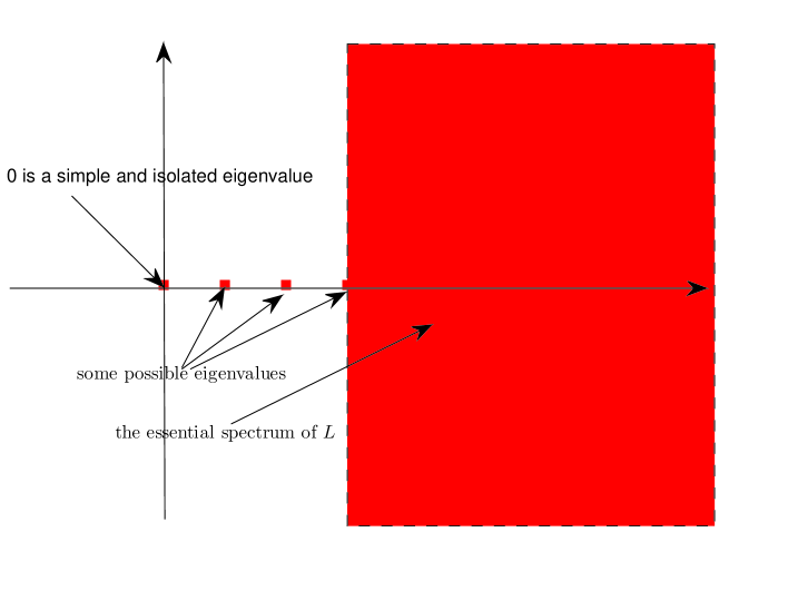
Figure 5.1: The Spectrum of $L$

The second approach is to use perturbation theory, which amounts to expanding $e^{-tL}$ in powers of the operator $K,$ (see  (3.7)):

$$e^{-tL}=e^{-t(\nu+v\cdot\nabla_{x})}+\int_{0}^{t}e^{-(t-s)(\nu+v\cdot\nabla_{x})}Ke^{-s(\nu+v\cdot\nabla_{x})}\ ds+\cdots.$$

It will be shown in Proposition  5.2 that each term in this expansion can be estimated quite well, but the fact that $K$ is unbounded forces us to estimate them in different spaces.

We will combine these two approaches to prove Theorem  5.1.

We expand the propagator $e^{-tL}(1-P_{0})$ using Duhamel’s principle:

$$e^{-tL}(1-P_{0})=\sum_{k=0}^{12}(1-P_{0})A_{k}(t)+(1-P_{0})\tilde{A}(t),$$ (5.3)

where the operators $A_{k}$ are defined recursively, with

$$A_{0}=A_{0}(t):=e^{-t(\nu+v\cdot\nabla_{x})},$$ (5.4)

and $A_{k},\ k=1,2,\cdots,12,$ given by

$$A_{k}(t):=\int_{0}^{t}e^{-(t-s)(\nu+v\cdot\nabla_{x})}KA_{k-1}(s)\ ds.$$ (5.5)

Finally $\tilde{A}$ is defined by

$$\tilde{A}(t)=\int_{0}^{t}e^{-(t-s)L}KA_{12}(s)\ ds.$$ (5.6)

The exact form of $A_{k},\ k=0,\ 1,\cdots,12,$ implies the following estimates.

Proposition 5.2.

There exist positive constants $C_{0}$ and $C_{1}$ such that, for any function $f:\ \mathbb{R}^{3}\times\mathbb{T}^{3}\rightarrow\mathbb{C},$

$$\|A_{k}(t)f\|_{L^{1}(\mathbb{R}^{3}\times\mathbb{T}^{3})}\leq C_{1}e^{-C_{0}t}\|\langle v\rangle^{k}f\|_{L^{1}(\mathbb{R}^{3}\times\mathbb{T}^{3})}.$$ (5.7)

This proposition is proven in Subsection  5.1.

The estimate on $\tilde{A}$, which, by definition, is given by

$$\tilde{A}=\int_{0}^{t}e^{-(t-s_{1})L}K\int_{0}^{s_{1}}e^{-(s_{1}-s_{2})(\nu+v\cdot\nabla_{x})}K\cdots\int_{0}^{s_{12}}e^{-(s_{12}-s_{13})(\nu+v\cdot\nabla_{x})}Ke^{-s_{13}(\nu+v\cdot\nabla_{x})}\ ds_{13}\cdots ds_{1},$$

is more involved.

We first transform $\tilde{A}$ to a more convenient form.

One of the important properties of the operators $L$ and $L_{0}$ is that, for any function $g:\ \mathbb{R}^{3}\rightarrow\mathbb{C}$ (i.e., independent of $x$) and ${\bf{n}}\in\mathbb{Z}^{3},$ we have that

$$\begin{array}[]{lll}P_{0}e^{i{\bf{n}}\cdot x}g&=&0\ \ \text{if}\ {\bf{n}}\not=0,\\ &&\\ Le^{i{\bf{n}}\cdot x}g&=&e^{i{\bf{n}}\cdot x}L_{{\bf{n}}}g,\\ &&\\ (\nu+v\cdot\nabla_{x})e^{i{\bf{n}}\cdot x}g&=&e^{i{\bf{n}}\cdot x}(\nu+i{\bf{n}}\cdot v)g,\end{array}$$ (5.8)

where the operator $L_{{\bf{n}}}$ is unbounded and defined as

$$L_{{\bf{n}}}:=\nu+i{\bf{n}}\cdot v+K.$$

(Recall that $P_{0}$ has been defined in  (5.1).)

To make  (5.8) applicable, we Fourier-expand the function $g:\ \mathbb{R}^{3}\times\mathbb{T}^{3}\rightarrow\mathbb{C}$ in the variable $x,$ i.e.,

$$g(v,x)=\sum_{{\bf{n}}\in\mathbb{Z}^{3}}e^{i{\bf{n}}\cdot x}g_{{\bf{n}}}(v).$$ (5.9)

Then  (4.14) and  (5.8) yield the bound

$$\|(1-P_{0})\tilde{A}g\|_{L^{1}(\mathbb{R}^{3}\times\mathbb{T}^{3})}\leq\sum_{{\bf{n}}\in\mathbb{Z}^{3}}\|\tilde{A}_{{\bf{n}}}g_{n}\|_{L^{1}(\mathbb{R}^{3})},$$ (5.10)

where $\tilde{A}_{{\bf{n}}}$ is defined as follows: If ${\bf{n}}\not=(0,0,0)$ then

$$\tilde{A}_{{\bf{n}}}:=\int_{0}^{t}e^{-(t-s_{1})L_{{\bf{n}}}}K\int_{0}^{s_{1}}e^{-(s_{1}-s_{2})(\nu+iv\cdot{\bf{n}})}K\cdots\int_{0}^{s_{12}}e^{-(s_{12}-s_{13})(\nu+iv\cdot{\bf{n}})}Ke^{-s_{13}(\nu+iv\cdot{\bf{n}})}\ ds_{13}\cdots ds_{1}$$

and for ${\bf{n}}=(0,0,0)$ we define

$$\tilde{A}_{0}:=\int_{0}^{t}(1-P_{0})e^{-(t-s_{1})L_{0}}K\int_{0}^{s_{1}}e^{-(s_{1}-s_{2})\nu}K\cdots\int_{0}^{s_{12}}e^{-(s_{12}-s_{13})\nu}Ke^{-s_{13}\nu}\ ds_{13}\cdots ds_{1}.$$

Next, we study $\tilde{A}_{{\bf{n}}}$, which is defined in terms of the operators $e^{-tL_{{\bf{n}}}}$, $e^{-t[\nu+i{\bf{n}}\cdot v]}$ and $Ke^{-t[\nu+i{\bf{n}}\cdot v]}K.$

It is easy to estimate $e^{-t[\nu+i{\bf{n}}\cdot v]}:$ The fact that the function $\nu$ has a positive global minimum $\Lambda$ (see  (3.9)) implies that

$$\|e^{-t[\nu+i{\bf{n}}\cdot v]}\|_{L^{1}\rightarrow L^{1}}\leq e^{-\Lambda t}.$$ (5.11)

We provide some rough estimate on the operator $e^{-tL_{{\bf{n}}}}$.

Lemma 5.3.

If ${\bf{n}}\not=(0,0,0)$ then there exist positive constants $C_{0}$ and $C_{1}$ such that

$$\|e^{-tL_{{\bf{n}}}}\|_{L^{1}(\mathbb{R}^{3})\rightarrow L^{1}(\mathbb{R}^{3})}\leq C_{1}(1+|{\bf{n}}|)e^{-C_{0}t}.$$ (5.12)

For ${\bf{n}}=(0,0,0)$

$$\|e^{-tL_{{\bf{0}}}}(1-P_{0})\|_{L^{1}(\mathbb{R}^{3})\rightarrow L^{1}(\mathbb{R}^{3})}\leq C_{1}e^{-C_{0}t}.$$ (5.13)

This lemma will be proven in Subsection  5.2.

The most important step is to estimate

$$K_{t}^{({\bf{n}})}:=Ke^{-t(\nu+i{\bf{n}}\cdot v)}K.$$

Let $K(v,u)$ be the integral kernel of $K$. Then the integral kernel, $K_{t}^{({\bf{n}})}(v,u),$ of $K_{t}^{({\bf{n}})}$ is given by

$$K_{t}^{({\bf{n}})}(v,u)=\int_{\mathbb{R}^{3}}K(v,z)e^{-t[\nu(z)+i{\bf{n}}\cdot z]}K(z,u)\ dz.$$

The presence of the factor $e^{-it{\bf{n}}\cdot z}$ plays an important role. It makes the operator $K_{t}^{({\bf{n}})}$ smaller, as $|{\bf{n}}|$ becomes larger.

Lemma 5.4.

There exist positive constants $C_{0}$ and $C_{1}$ such that, for any ${\bf{n}}\in\mathbb{Z}^{3},$

$$\|K_{t}^{({\bf{n}})}f\|_{L^{1}(\mathbb{R}^{3})}\leq\frac{C_{1}}{1+|{\bf{n}}|t}e^{-C_{0}t}\|\langle v\rangle^{3}f\|_{L^{1}(\mathbb{R}^{3})}.$$ (5.14)

This lemma will be proven in Subsection  5.3.

The results in Proposition  5.2, Lemma  5.3 and Lemma  5.4 suffice to prove Theorem  5.1.
Proof of Theorem  5.1. In Equation  (5.3) we have decomposed $e^{-tL}(1-P_{0})$ into several terms. The operators $A_{k},\ k=0,1,2,\cdots,12,$ are estimated in Proposition  5.2.

In what follows, we study $\tilde{A}$. By  (5.10) we only need to control $\tilde{A}_{{\bf{n}}},\ {\bf{n}}\in\mathbb{Z}^{3}$. For ${\bf{n}}=(0,0,0)$ it is easy to see that

$$\|\tilde{A}_{0}g_{{\bf{0}}}\|_{L^{1}(\mathbb{R}^{3})}\lesssim e^{-C_{0}t}\|\langle v\rangle^{12}g_{\bf{0}}\|_{L^{1}(\mathbb{R}^{3})}$$ (5.15)

by collecting the different estimates in  (5.11) and Lemma  5.3 and using the estimates on $K=-K_{0}+C_{\infty}\kappa K_{1}$ in Lemma  3.1.

For ${\bf{n}}\not=0$, we observe that the integrands in the definitions of $\tilde{A}_{{\bf{n}}}$ are products of terms $e^{-(t-s_{1})L_{{\bf{n}}}},$ $Ke^{-(s_{k}-s_{k+1})(\nu+i{\bf{n}}\cdot v)}K$ and $e^{-(s_{k}-s_{k+1})(\nu+i{\bf{n}}\cdot v)}$, where $k\in\{1,2,\cdots,13\}$ (we use the convention that $s_{14}=0$). Applying the bounds in  (5.11), Lemma  5.3 and Lemma  5.4, we see that there is a constant $C_{0}>0$ such that

$$\begin{array}[]{lll}&&\|\tilde{A}_{{\bf{n}}}g_{\bf{n}}\|_{L^{1}(\mathbb{R}^{3})}\\ &&\\ &\lesssim&e^{-C_{0}t}(1+|{\bf{n}}|)\|\langle v\rangle^{20}g_{\bf{n}}\|_{L^{1}(\mathbb{R}^{3})}\times\\ &&\\ &&\int_{0}^{t}\int_{0}^{s_{1}}\cdots\int_{0}^{s_{12}}[1+|{\bf{n}}|(s_{12}-s_{13})]^{-1}[1+|{\bf{n}}|(s_{8}-s_{11})]^{-1}\cdots[1+|{\bf{n}}|(s_{2}-s_{3})]^{-1}\ ds_{13}ds_{12}\cdots ds_{1}.\end{array}$$

By direct computation we find that there exists a positive constant $\tilde{C}_{0}\leq C_{0}$ such that

$$\|\tilde{A}_{{\bf{n}}}g_{\bf{n}}\|_{L^{1}(\mathbb{R}^{3})}\lesssim e^{-\tilde{C}_{0}t}\frac{1}{(1+|{\bf{n}}|)^{4}}\|\langle v\rangle^{20}g_{\bf{n}}\|_{L^{1}(\mathbb{R}^{3})}.$$

Plugging this and  (5.15) into  (5.10), we find that

$$\|(1-P_{0})\tilde{A}g\|_{L^{1}(\mathbb{R}^{3}\times\mathbb{T}^{3})}\lesssim e^{-\tilde{C}_{0}t}\sum_{{\bf{n}}\in\mathbb{Z}^{3}}\frac{1}{(1+|{\bf{n}}|)^{4}}\|\langle v\rangle^{20}g_{{\bf{n}}}\|_{L^{1}(\mathbb{R}^{3})}.$$ (5.16)

The terms on the right hand side are bounded by

$$\|\langle v\rangle^{20}g_{{\bf{n}}}\|_{L^{1}(\mathbb{R}^{3})}\leq(2\pi)^{3}\|\langle v\rangle^{20}g\|_{L^{1}(\mathbb{R}^{3}\times\mathbb{T}^{3})}.$$

This, together with the fact that $\displaystyle\sum_{{\bf{n}}\in\mathbb{Z}^{3}}\frac{1}{(1+|{\bf{n}}|)^{4}}<\infty,$ implies that

$$\|(1-P_{0})\tilde{A}g\|_{L^{1}(\mathbb{R}^{3}\times\mathbb{T}^{3})}\lesssim e^{-\tilde{C}_{0}t}\|\langle v\rangle^{20}g\|_{L^{1}(\mathbb{R}^{3}\times\mathbb{T}^{3})}.$$ (5.17)

Obviously Equation  (5.3), Inequality  (5.17) and Proposition  5.2 imply Theorem  5.1.

$\square$

5.1 Proof of Proposition  5.2

Recall the meaning of the constant $\Lambda$ in  (3.9). The definition of $A_{0}$ (see  (5.4)) implies that

$$\|A_{0}(t)f\|_{L^{1}(\mathbb{R}^{3}\times\mathbb{T}^{3})}\leq e^{-\Lambda t}\|f\|_{L^{1}(\mathbb{R}^{3}\times\mathbb{T}^{3})}.$$ (5.18)

For $A_{1},$ we use the estimate for the unbounded operator $K$ given in Lemma  3.1. A direct computation then yields

$$\begin{array}[]{lll}\|A_{1}(f)\|_{L^{1}(\mathbb{R}^{3}\times\mathbb{T}^{3})}&\leq&\int_{0}^{t}e^{-\Lambda(t-s)}\|Ke^{-s(\nu+v\cdot\nabla_{x})x}f\|_{L^{1}(\mathbb{R}^{3}\times\mathbb{T}^{3})}\ ds\\ &&\\ &\lesssim&\int_{0}^{t}e^{-\Lambda(t-s)}e^{-\Lambda s}\ ds\|\langle v\rangle f\|_{L^{1}}\\ &&\\ &=&e^{-\Lambda t}t\|\langle v\rangle f\|_{L^{1}}.\end{array}$$

Similar arguments yield the desired estimates for $A_{k},\ k=2,3,\cdots 12$.

Thus, the proof of Proposition  5.2 is complete.

$\square$

5.2 Proof of Lemma  5.3

Proof.

If ${\bf{n}}=(0,0,0)$ then the proof of  (5.12) is similar to that of a similar estimate in  [1, 31, 26] and to the proof of  (5.13) given below. It is therefore omitted. What makes the present situation different to the one considered in  [1, 31, 26] is that the spectrum of the linear operator $L_{{\bf{n}}}$ depends on ${\bf{n}}$ in a non-trivial manner. The union over ${\bf{n}}$ of the spectra of the operators $L_{\bf{n}}$ fills almost the entire right half of the complex plane.

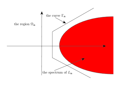
Figure 5.2: The spectrum of $L_{{\bf{n}}}$, the curve $\Gamma_{{\bf{n}}},$ and the region $\Omega_{{\bf{n}}}$

For any ${\bf{n}}\in\mathbb{Z}^{3},$ we define a curve $\Gamma_{{\bf{n}}}$ (see Figure  5.2),

$$\Gamma_{{\bf{n}}}:=\Gamma_{1}({\bf{n}})\cup\Gamma_{2}({\bf{n}})\cup\Gamma_{3}({\bf{n}})$$ (5.19)

with

$$\Gamma_{1}({\bf{n}}):=\{\Theta+i\beta|\ \beta\in[-\Psi(|{\bf{n}}|+1),\ \Psi(|{\bf{n}}|+1)]\};$$

$$\Gamma_{2}({\bf{n}}):=\{\Theta+i(|{\bf{n}}|+1)\Psi+\beta+i\Psi\beta(|{\bf{n}}|+1),\ \beta\geq 0\};$$

$$\Gamma_{3}({\bf{n}}):=\{\Theta-i(|{\bf{n}}|+1)\Psi+\beta-i\Psi\beta(|{\bf{n}}|+1),\ \beta\geq 0\}.$$

Here $\Theta$ and $\Psi$ are positive constants to be chosen later; they are independent of the constant $\kappa$ in  (2.1).

Moreover, we define $\Omega_{{\bf{n}}}$ to be the complement of the region encircled by the curve $\Gamma_{{\bf{n}}};$ see Figure  5.2.

The following lemma provides an important estimate.

Lemma 5.5.

Suppose that the positive constants $\Theta$ and $\frac{1}{\Psi}$ are chosen sufficiently small. Then there exists a constant $C$ independent of ${\bf{n}}$ such that, for any point $\zeta\in\Omega_{{\bf{n}}}$ and ${\bf{n}}\in\mathbb{Z}^{3}\backslash\{(0,0,0)\},$ we have

$$\|(L_{{\bf{n}}}-\zeta)^{-1}\|_{L^{1}\rightarrow L^{1}}\leq C.$$

This lemma is proven in Appendix  B.

This lemma and the spectral theorem in  [28] yield the formula

$$e^{-tL_{{\bf{n}}}}=\frac{1}{2\pi i}\oint_{\Gamma_{{\bf{n}}}}e^{-t\zeta}[\zeta-L_{{\bf{n}}}]^{-1}\ d\zeta$$ (5.20)

on $L^{1}(\mathbb{R}^{3}).$ Applying Lemma  5.5 to  (5.20) we obtain that

$$\|e^{-tL_{{\bf{n}}}}\|_{L^{1}\rightarrow L^{1}}\lesssim\int_{\zeta\in\Gamma_{1}({\bf{n}})\cup\Gamma_{2}({\bf{n}})\cup\Gamma_{3}({\bf{n}})}e^{-tRe\ \zeta}\ |d\zeta|$$

By the definition of $\Gamma_{1}({\bf{n}})$, it is easy to see that

$$\int_{\zeta\in\Gamma_{1}}e^{-\Theta t}|d\zeta|\lesssim e^{-\Theta t}|{\bf{n}}|.$$

Similarly, the definitions of $\Gamma_{2}({\bf{n}})$ and $\Gamma_{3}({\bf{n}})$ imply that for any $t\geq 1,$

$$\int_{\zeta\in\Gamma_{2}({\bf{n}})\cup\Gamma_{3}({\bf{n}})}e^{-tRe\zeta}\ |d\zeta|\lesssim(1+|{\bf{n}}|)\int_{\Theta}^{\infty}e^{-t\sigma}d\sigma\lesssim e^{-\Theta t}(1+|{\bf{n}}|).$$

Collecting the estimates above, we arrive at  (5.12), provided that $t\geq 1.$

The proof will be complete if we can show that the propagator $e^{-tL_{{\bf{n}}}}$ is bounded on $L^{1}(\mathbb{R}^{3})$ when $t\in[0,1].$ To prove this, we establish the local wellposedness of the equation

$$\begin{array}[]{lll}\partial_{t}g&=&[-\nu-i{\bf{n}}\cdot v+K]g,\\ g(v,0)&=&g_{0}(v).\end{array}$$

This is easier to prove than local wellposedness of the nonlinear equation in Proposition  4.1, and we permit ourselves to omit the details.

This completes the proof of Lemma  5.3. ∎

5.3 Proof of Inequality ( 5.14)

Proof.

We denote the integral kernel of the operator $K$ by $K(v,u)$ and infer its explicit form from  (3.7),  (3.4) and  (3.6). It is then easy to see that the integral kernel of the operator $Ke^{-t(\nu+i{\bf{n}}\cdot v)}K$ is given by

$$K_{t}^{({\bf{n}})}(v,u):=\int_{\mathbb{R}^{3}}K(v,z)e^{-t[\nu(z)+i{\bf{n}}\cdot z]}K(z,u)\ d^{3}z.$$

We use the oscillatory nature of $e^{-it{\bf{n}}\cdot z}$ to derive some “smallness estimates” when $|{\bf{n}}|$ is sufficiently large. Mathematically, we achieve this by integrating by parts in the variable $z$. Without loss of generality we assume that

$$|n_{1}|\geq\frac{1}{3}|{\bf{n}}|.$$

We then integrate by parts in the variable $z_{1}$ to obtain

$$\begin{array}[]{lll}K_{t}^{({\bf{n}})}(v,u)&=&\int_{\mathbb{R}^{3}}K(v,z)K(z,u)\frac{1}{-t[\partial_{z_{1}}\nu(z)+in_{1}]}\partial_{z_{1}}e^{-t[\nu(z)+i{\bf{n}}\cdot z]}\ d^{3}z\\ &&\\ &=&\int_{\mathbb{R}^{3}}\partial_{z_{1}}[K(v,z)K(z,u)\frac{1}{t[\partial_{z_{1}}\nu(z)+in_{1}]}]e^{-t[\nu(z)+i{\bf{n}}\cdot z]}\ d^{3}z\end{array}$$ (5.21)

The different terms in $\partial_{z_{1}}[K(v,z)K(z,u)\frac{1}{t[\partial_{z_{1}}\nu(z)+in_{1}]}]$ are dealt with as follows.

• We claim that, for $l=0,1,$

  $$\int_{\mathbb{R}^{3}}\langle v\rangle^{m}|\partial_{z_{1}}^{l}K(v,z)|\ d^{3}v\lesssim\langle z\rangle^{m+2},\ \ \int_{\mathbb{R}^{3}}\langle z\rangle^{m}|\partial_{z_{1}}^{l}K(z,u)|\ d^{3}z\lesssim\langle u\rangle^{m+2}.$$ (5.22)

• By direct computation,

  $$|\partial_{z}^{l}\frac{1}{t[\partial_{z_{1}}\nu(z)+in_{1}]}|\lesssim\frac{1}{|{\bf{n}}|t}\ \text{for}\ l=0,1.$$ (5.23)

These bounds and the fact that $e^{-t\nu}\lesssim e^{-\Lambda t}$ (see  (3.9)) imply that

$$\int_{\mathbb{R}^{3}\times\mathbb{R}^{3}}\langle v\rangle^{m}|K_{t}^{({\bf{n}})}(v,u)g(u)|\ d^{3}u\lesssim\frac{e^{-\Lambda t}}{|{\bf{n}}|t}\|\langle v\rangle^{m+3}g\|_{L^{1}}.$$

To remove the non-integrable singularity in the upper bound at $t=0$, we use a straightforward estimate derived from the definition of $K_{t}^{({\bf{n}})}$ to obtain

$$\int_{\mathbb{R}^{3}\times\mathbb{R}^{3}}\langle v\rangle^{m}|K_{t}^{({\bf{n}})}(v,u)g(u)|\ d^{3}u\lesssim e^{-\Lambda t}\|\langle v\rangle^{m+3}g\|_{L^{1}}.$$

Combination of these two estimates yields  (5.14).

We are left with proving  (5.22). In the next we focus on proving  (5.22) when $l=1$, the case $l=0$ is easier, hence omitted. By direct computation we find that

$$\begin{array}[]{lll}|\partial_{z_{1}}K(v,z)|&\lesssim&\kappa|\partial_{z_{1}}|z-v|^{-1}e^{-\frac{|(z-v)\cdot v|^{2}}{|z-v|^{2}}}|+\kappa|\partial_{z_{1}}|z-v|e^{-|v|^{2}}|+|\partial_{z_{1}}r_{0}(z,v)|\end{array}$$

and, similarly, that

$$|\partial_{z_{1}}K(z,u)|\lesssim\kappa|\partial_{z_{1}}|z-u|^{-1}e^{-\frac{|(z-u)\cdot z|^{2}}{|z-u|^{2}}}|+\kappa|\partial_{z_{1}}|z-u|e^{-|z|^{2}}|+|\partial_{z_{1}}r_{0}(u,z)|.$$

Among the various terms we only study the most difficult one, namely $\partial_{z_{1}}K_{1,1}(v,z)$, where $K_{1,1}(v,z)$ is defined by

$$K_{1,1}(v,z):=|z-v|^{-1}e^{-\frac{|(z-v)\cdot v|^{2}}{|z-v|^{2}}}.$$

By direct computation

$$|\partial_{z_{1}}K_{1,1}(v,z)|\lesssim\frac{1+|v_{1}|}{|v-z|^{2}}e^{-\frac{1}{2}\frac{|(z-v)\cdot v|^{2}}{|z-v|^{2}}}.$$

To complete our estimate we divide the set $(v,z)\in\mathbb{R}^{3}\times\mathbb{R}^{3}$ into two subsets defined by $|v|\leq 10|z|$ and $|v|>10|z|,$ respectively. In the first subset we have that

$$|\partial_{z_{1}}K_{1,1}(v,z)|\lesssim\frac{1}{|v-z|^{2}}(|v|+1)\leq\frac{10(|z|+1)}{|v-z|^{2}},$$

and hence

$$\int_{|v|\leq 8|z|}\langle v\rangle^{m}|\partial_{z_{1}}K_{1,1}(v,z)|\ d^{3}v\leq 10(1+|z|)^{m+1}\int_{|v|\leq 10|z|}\frac{1}{|v-z|^{2}}\ d^{3}v\lesssim(1+|z|)^{m+2}.$$ (5.24)

In the second subset we have that $z-v\approx-v$, which implies that $\frac{|(z-v)\cdot v|}{|z-v|}\geq\frac{1}{2}|v|$. Thus,

$$|\partial_{z_{1}}K_{1,1}(v,z)|\leq\frac{1+|v|}{|v|^{2}}e^{-\frac{1}{8}|v|^{2}}.$$

This obviously implies that

$$\int_{|v|\geq 10|z|}\langle v\rangle^{m}|\partial_{z_{1}}K_{1,1}(v,z)|\ d^{3}v\lesssim\int_{|v|\geq 10|z|}\langle v\rangle^{m}\frac{1+|v|}{|v|^{2}}\ e^{-\frac{1}{8}|v|^{2}}d^{3}v\lesssim 1.$$ (5.25)

By such estimates the proof of  (5.22) can be easily completed. ∎

6 Proof of the Main Theorem

To simplify notations, we let $L^{1}$ stand for $L^{1}(\mathbb{R}^{3}\times\mathbb{T}^{3})$.

Given a solution, $f(\cdot,s)$, $0\leq s\leq t$, of the Boltzmann equation  (3.2), we introduce two “control functions”, $\mathcal{M}$ and $\mathcal{I}$:

$$\begin{array}[]{lll}\mathcal{M}(t)&:=&\displaystyle\max_{0\leq s\leq t}e^{C_{0}s}\sum_{|\alpha|\leq 8}\|\partial_{x}^{\alpha}f(s)\|_{L^{1}},\\ &&\\ \mathcal{I}(t)&:=&\displaystyle\sum_{|\alpha|\leq 8}\int_{0}^{t}\|\langle v\rangle^{2m+2}\partial_{x}^{\alpha}f(s)\|_{L^{1}}\ ds,\end{array}$$ (6.1)

where, the constants $m$ and $C_{0}$ are as in Theorem  5.1.

These two functions can be estimated as follows.

Lemma 6.1.

$$\mathcal{M}(t)\leq C[\sum_{|\alpha|\leq 8}\|\langle v\rangle^{m}\partial_{x}^{\alpha}f_{0}\|_{L^{1}}+\kappa\mathcal{M}^{\frac{3}{2}}\mathcal{I}^{\frac{1}{2}}];$$ (6.2)

and

$$\mathcal{I}(t)\leq C[\sum_{|\alpha|\leq 8}\|\langle v\rangle^{2m+1}\partial_{x}^{\alpha}f_{0}\|_{L^{1}}+\kappa\mathcal{I}(t)\mathcal{M}(t)+\mathcal{M}(t)].$$ (6.3)

for a finite constant $C$, where $f_{0}$ is the initial condition.

This lemma will be proven below.

We are now ready to prove our main result, Theorem  2.1.
Proof of Theorem  2.1 By local wellposedness of the equation, there exists a time interval $[0,T]$, $T=T(\kappa),$ such that

$$\mathcal{M}(t)\leq\kappa^{-\frac{1}{4}},\ \text{for any time}\ t\in[0,T].$$ (6.4)

We move the term $C\kappa\mathcal{I}(t)\mathcal{M}(t)$ on the right hand side of  (6.3) to the left hand side and then use the fact that $C\kappa\mathcal{M}(t)\leq\frac{1}{2}$ to conclude that

$$\mathcal{I}(t)\leq 2C[\sum_{|\alpha|\leq 8}\|\langle v\rangle^{2m}\partial_{x}^{\alpha}f_{0}\|_{L^{1}}+\mathcal{M}(t)].$$ (6.5)

Plugging this bound into the right hand side of  (6.2) and using  (6.4), we obtain that

$$\mathcal{M}(t)\leq C(\sum_{|\alpha|\leq 8}\|\langle v\rangle^{m}\partial_{x}^{\alpha}f_{0}\|_{L^{1}}+\kappa^{\frac{1}{2}}\mathcal{M}(t)).$$

This, together with the fact $C\kappa^{\frac{1}{2}}\leq\frac{1}{2},$ implies that

$$\mathcal{M}(t)\leq 2C\sum_{|\alpha|\leq 8}\|\langle v\rangle^{m}\partial_{x}^{\alpha}f_{0}\|_{L^{1}},\ \text{for any time}\ t\in[0,T].$$ (6.6)

This in turn implies that  (6.4) holds on a larger time interval. By running the arguments  (6.4)- (6.6) iteratively we find that  (6.6) holds on the time interval $[0,\infty).$

Using the definition of $\mathcal{M}$, in  (6.1), we obtain that, for any time $t\in[0,\infty),$

$$\sum_{|\alpha|\leq 8}\|\partial_{x}^{\alpha}f(t)\|_{L^{1}}\leq 2Ce^{-C_{0}t}\sum_{|\alpha|\leq 8}\|\langle v\rangle^{m}\partial_{x}^{\alpha}f_{0}\|_{L^{1}},$$ (6.7)

which together with the definition of $f$, see  (3.1), implies inequality  (2.5) in Theorem  2.1.

The proof of Theorem  2.1 is complete.

$\square$

6.1 Proof of Lemma  6.1

Proof.

We apply Duhamel’s principle to rewrite the Boltzmann equation  (3.2) as

$$f=e^{-tL}(1-P_{0})f_{0}+\kappa\int_{0}^{t}e^{-(t-s)L}(1-P_{0})Q(f,f)(s)\ ds,$$

Here, the fact that $(1-P_{0})f=f$, which is implied by  (3.1) and the definition of $P_{0}$ in  (5.1), has been used. We apply the propagator estimate in Theorem  5.1 to conclude that, for any $\alpha\in(\mathbb{Z}^{+})^{3}$ with $|\alpha|\leq 8,$

$$\begin{array}[]{lll}\|\partial_{x}^{\alpha}f(\cdot,t)\|_{L^{1}}&\lesssim&e^{-C_{0}t}\|\langle v\rangle^{m}\partial_{x}^{\alpha}f_{0}\|_{L^{1}}+\kappa\int_{0}^{t}e^{-C_{0}(t-s)}\|\langle v\rangle^{m}\partial_{x}^{\alpha}Q(f,f)(s)\|_{L^{1}}\ ds\end{array}$$ (6.8)

To estimate the nonlinear term on the right hand side, we use techniques similar to those in  (4.5) to obtain

$$\begin{array}[]{lll}\|\langle v\rangle^{m}\partial_{x}^{\alpha}Q(f,f)\|_{L^{1}}&\lesssim&\displaystyle\sum_{l=0}^{m}\sum_{|\beta_{1}|\leq 8}\|\langle v\rangle^{k}\partial_{x}^{\beta_{1}}f\|_{L{1}}\sum_{|\beta_{2}|\leq 8}\|\langle v\rangle^{m+1-k}\partial_{x}^{\beta_{2}}f\|_{L^{1}}\\ &&\\ &\lesssim&\displaystyle\sum_{|\beta_{1}|,\ |\beta_{2}|\leq 8}\|\langle v\rangle^{m+1}\partial_{x}^{\beta_{1}}f\|_{L^{1}}\|\partial_{x}^{\beta_{2}}f\|_{L^{1}}.\end{array}$$

To the term $\|\langle v\rangle^{m}\partial_{x}^{\beta_{1}}f\|_{L^{1}}$ on the right hand side we apply the Schwarz inequality to obtain

$$\|\langle v\rangle^{m+1}\partial_{x}^{\beta}f\|_{L^{1}}^{2}\leq\|\langle v\rangle^{2m+2}\partial_{x}^{\beta}f\|_{L^{1}}\|\partial_{x}^{\beta}f\|_{L^{1}}.$$

Plugging this into  (6.8), we obtain that

$$\|\partial_{x}^{\alpha}f\|_{L^{1}}\lesssim e^{-C_{0}t}\|\langle v\rangle^{m}\partial_{x}^{\alpha}f_{0}\|_{L^{1}}+\displaystyle\kappa\sum_{|\beta_{1}|,\ |\beta_{2}|\leq 8}\int_{0}^{t}e^{-C_{0}(t-s)}\|\langle v\rangle^{2m+2}\partial_{x}^{\beta_{1}}f\|_{L^{1}}^{\frac{1}{2}}\|\partial_{x}^{\beta_{2}}f\|_{L^{1}}^{\frac{3}{2}}\ ds$$

Applying the Schwarz inequality again and using the definitions of $\mathcal{M}$ and $\mathcal{I},$ we find that

$$\begin{array}[]{lll}\|\partial_{x}^{\alpha}f\|_{L^{1}}&\lesssim&e^{-C_{0}t}\|\langle v\rangle^{m}\partial_{x}^{\alpha}f_{0}\|_{L^{1}}+\displaystyle\sum_{|\beta_{1}|,\ |\beta_{2}|\leq 8}\kappa[\int_{0}^{t}e^{-2C_{0}(t-s)}\|\partial_{x}^{\beta_{1}}f\|_{L^{1}}^{3}\ ds]^{\frac{1}{2}}[\int_{0}^{t}\|\langle v\rangle^{2m+2}\partial_{x}^{\beta_{2}}f\|_{L^{1}}\ ds]^{\frac{1}{2}}\\ &&\\ &\leq&e^{-C_{0}t}\|\langle v\rangle^{m}\partial_{x}^{\alpha}f_{0}\|_{L^{1}}+\kappa e^{-C_{0}t}\mathcal{M}^{\frac{3}{2}}\mathcal{I}^{\frac{1}{2}}.\end{array}$$

Recalling the definition of $\mathcal{M},$ we see that the proof of  (6.2) is complete.

To prove  (6.3), or to estimate $\int_{0}^{t}\|\langle v\rangle^{2m+2}f(s)\|_{L^{1}}\ ds,$ we rewrite  (3.2) as

$$\partial_{x}^{\alpha}f(t)=e^{-t(\nu+v\cdot\nabla_{x})}\partial_{x}^{\alpha}f_{0}+\int_{0}^{t}e^{-(t-s)(\nu+v\cdot\nabla_{x})}\partial_{x}^{\alpha}H(s)\ ds,$$

where $H(s)$ is defined by

$$H(s):=K_{0}f(s)+\kappa K_{1}f(s)+\kappa Q(f,f)(s).$$

By direct computation and the fact that $L^{1}$-norm is preserved under the mapping $e^{-tv\cdot\nabla_{x}}$ we obtain

$$\begin{array}[]{lll}\|\langle v\rangle^{2m+2}\partial_{x}^{\alpha}f(t)\|_{L^{1}}&\leq&\|\langle v\rangle^{2m+2}e^{-t[\nu+v\cdot\nabla_{x}]}\partial_{x}^{\alpha}f_{0}\|_{L^{1}}+\int_{0}^{t}\|\langle v\rangle^{2m+2}e^{-(t-s)[\nu+v\cdot\nabla_{x}]}\partial_{x}^{\alpha}H(s)\|_{L^{1}}\ ds\\ &&\\ &=&\|\langle v\rangle^{2m+2}e^{-t\nu}\partial_{x}^{\alpha}f_{0}\|_{L^{1}}+\int_{0}^{t}\|\langle v\rangle^{2m+2}e^{-(t-s)\nu}\partial_{x}^{\alpha}H(s)\|_{L^{1}}\ ds\end{array}$$

Integrate both sides from $0$ to $t$, and use the obvious fact that $\int_{0}^{t}\|g(s)\|_{L^{1}}\ ds=\|\int_{0}^{t}|g|(s)\ ds\|_{L^{1}}$ we arrive at

$$\int_{0}^{t}\|\langle v\rangle^{2m+2}\partial_{x}^{\alpha}f(s)\|_{L^{1}}\ ds\leq\|\int_{0}^{t}\langle v\rangle^{2m+2}e^{-s\nu}|\partial_{x}^{\alpha}f_{0}|\ ds\|_{L^{1}}+\|\int_{0}^{t}\int_{0}^{s}\langle v\rangle^{2m+2}e^{-(s-s_{1})\nu}|\partial_{x}^{\alpha}H(s_{1})|\ ds_{1}ds\|_{L^{1}}.$$

The first term on the right hand side can be integrated explicitly. For the second term, we integrate by parts in the variable $s$. We find that

$$\begin{array}[]{lll}\int_{0}^{t}\|\langle v\rangle^{2m+2}\partial_{x}^{\alpha}f(s)\|_{L^{1}}\ ds&\leq&\|\nu^{-1}\langle v\rangle^{2m+2}\partial_{x}^{\alpha}f_{0}\|_{L^{1}}+\int_{0}^{t}\|\nu^{-1}\langle v\rangle^{2m+2}\partial_{x}^{\alpha}H(s)\|_{L^{1}}\ ds\\ &&\\ &\lesssim&\|\langle v\rangle^{2m+1}\partial_{x}^{\alpha}f_{0}\|_{L^{1}}+\int_{0}^{t}\|\langle v\rangle^{2m+1}\partial_{x}^{\alpha}H(s)\|_{L^{1}}\ ds.\end{array}$$ (6.9)

In the last step we use the estimate for $\nu=\nu_{0}+C_{\infty}\kappa\nu_{1}$ in  (B.5), which, through its definition, makes it necessary to require that $r_{0}$ in  (2.1) be unbounded.

This together with the definition of $H$, the estimates on $K_{0}$ and $K_{1}$ in Lemma  3.1 and on the nonlinearity in  (4.13), implies that there exist constants $C_{1}$ and $C_{2}$ such that

$$\begin{array}[]{lll}&&\int_{0}^{t}\|\langle v\rangle^{2m+2}\partial_{x}^{\alpha}f(s)\|_{L^{1}}\ ds\\ &&\\ &\leq&C_{1}[\|\langle v\rangle^{2m+1}\partial_{x}^{\alpha}f_{0}\|_{L^{1}}+C_{\infty}\kappa\int_{0}^{t}\|\langle v\rangle^{2m+1}K_{1}\partial_{x}^{\alpha}f(s)\|_{L^{1}}\ ds\\ &&\\ &&+\int_{0}^{t}\|\langle v\rangle^{2m+1}K_{0}\partial_{x}^{\alpha}f(s)\|_{L^{1}}\ ds+\kappa\int_{0}^{t}\|\langle v\rangle^{2m+1}\partial_{x}^{\alpha}Q(f,f)(s)\|_{L^{1}}\ ds\\ &&\\ &\leq&C_{2}[\|\langle v\rangle^{2m+1}\partial_{x}^{\alpha}f_{0}\|_{L^{1}}+\kappa C_{\infty}\int_{0}^{t}\|\langle v\rangle^{2m+2}\partial_{x}^{\alpha}f(s)\|_{L^{1}}\ ds\\ &&\\ &&+\int_{0}^{t}\|\langle v\rangle\partial_{x}^{\alpha}f(s)\|_{L^{1}}\ ds+\kappa\displaystyle\sum_{|\beta_{1}|,\ |\beta_{2}|\leq 8}\int_{0}^{t}\|\langle v\rangle^{2m+2}\partial_{x}^{\beta_{1}}f(s)\|_{L^{1}}\|\partial_{x}^{\beta_{2}}f(s)\|_{L^{1}}\ ds].\end{array}$$ (6.10)

We use the Schwarz inequality to estimate the third term, $\int_{0}^{t}\|\langle v\rangle\partial_{x}^{\alpha}f(s)\|_{L^{1}}\ ds,$ on the right hand side:

$$C_{2}\int_{0}^{t}\|\langle v\rangle\partial_{x}^{\alpha}f(s)\|_{L^{1}}\ ds\leq\frac{1}{2}\int_{0}^{t}\|\langle v\rangle^{2m+2}\partial_{x}^{\alpha}f(s)\|_{L^{1}}\ ds+C_{3}(m)\int_{0}^{t}\|\partial_{x}^{\alpha}f(s)\|_{L^{1}}\ ds,$$

for any $m\geq 0$ with $C_{3}(m)\geq 0$.

Inserting this in  (6.10) and using that $\kappa>0$ is a small constant, we find that

$$\int_{0}^{t}\|\langle v\rangle^{2m+2}\partial_{x}^{\alpha}f(s)\|_{L^{1}}\ ds\lesssim\|\langle v\rangle^{2m+1}\partial_{x}^{\alpha}f_{0}\|_{L^{1}}+\kappa\displaystyle\sum_{|\beta|\leq 8}\int_{0}^{t}\|\langle v\rangle^{2m+2}\partial_{x}^{\beta}f(s)\|_{L^{1}}\ ds\mathcal{M}(t)+\mathcal{M}(t),$$

which together with the definition of $\mathcal{I}$ in  (6.1) implies the desired estimate  (6.3). ∎

Appendix A Proof of Lemma  3.1

It is easy to derive  (3.9) and  (3.10) by the definitions of $\nu_{0},\ \nu_{1}$ and $K_{0}$. We therefore omit the details.

We start with  (3.12). By direct computation

$$\begin{array}[]{lll}\|\langle v\rangle^{m}Q(f,g)\|_{L^{1}(\mathbb{R}^{3})}&=&\int_{\mathbb{R}^{3}\times\mathbb{R}^{3}\times\mathbb{S}^{2}}\langle v\rangle^{m}|(u-v)\cdot\omega|f(u^{\prime})|g|(v^{\prime})\ d^{3}ud^{3}vd^{2}\omega\\ &&\\ &&+\int_{\mathbb{R}^{3}\times\mathbb{R}^{3}\times\mathbb{S}^{2}}\langle v\rangle^{m}|(u-v)\cdot\omega|f(u)|g|(v)\ d^{3}ud^{3}vd^{2}\omega.\end{array}$$ (A.1)

It is easy to control the second term on the right hand side.

We then turn to the first term. For any fixed $\omega\in\mathbb{S}^{2},$ the mapping from $(u,v)\in\mathbb{R}^{6}$ to $(u^{\prime},v^{\prime})\in\mathbb{R}^{6}$ is a linear symplectic transformation, hence

$$d^{3}ud^{3}v=d^{3}u^{\prime}d^{3}v^{\prime}$$ (A.2)

where, $u^{\prime}$ and $v^{\prime}$ are defined  (2.1). This together with the observation that

$$\langle v\rangle^{m}\lesssim\langle u^{\prime}\rangle^{m}+\langle v^{\prime}\rangle^{m},\ \text{and}\ |(u-v)\cdot\omega|\lesssim|u^{\prime}|+|v^{\prime}|$$ (A.3)

and  (A.1) obviously implies  (3.12).

As one can infer from the definition $K_{1}$ in  (3.2),  (3.11) is a special case of  (3.12) by setting $f$ or $g$ to be $M=e^{-|v|^{2}}.$

$\square$

Appendix B Proof of Lemma  5.5

We start by simplifying the problem. Using the definitions of the operators $L_{{\bf{n}}}$, ${\bf{n}}\in\mathbb{Z}^{3}$, in  (5.8), $K$ in  (3.7), and $\nu$ in  (3.8) we find that

$$L_{{\bf{n}}}=\nu_{0}-K_{0}+i{\bf{n}}\cdot v+C_{\infty}\kappa[\nu_{1}+K_{1}].$$

The smallness of the constant $\kappa$ suggests to consider $\nu_{0}-K_{0}+i{\bf{n}}\cdot v$ as the dominant part. We then convert the estimate on $L_{{\bf{n}}}-\zeta$ to one on $\nu_{0}-K_{0}+i{\bf{n}}\cdot v-\zeta$.

To render this idea mathematically rigorous, we show that, in order to prove invertibility of $L_{{\bf{n}}}-\zeta,\ \zeta\in\Omega_{{\bf{n}}},$ it is sufficient to prove this property for $1-K_{\zeta,{\bf{n}}}$, with $K_{\zeta,{\bf{n}}}$ defined by

$$K_{\zeta,{\bf{n}}}:=K_{0}(\nu_{0}+i{\bf{n}}\cdot v-\zeta)^{-1}.$$ (B.1)

We rewrite $L_{{\bf{n}}}-\zeta$ as follows:

$$\begin{array}[]{lll}L_{{\bf{n}}}-\zeta&=&[1-K_{\zeta,{\bf{n}}}+C_{\infty}\kappa(\nu_{1}+K_{1})(\nu_{0}+i{\bf{n}}\cdot v-\zeta)^{-1}](\nu_{0}+i{\bf{n}}\cdot v-\zeta)\\ &&\\ &=&(1-K_{\zeta,{\bf{n}}})[1+C_{\infty}\kappa(1-K_{\zeta,{\bf{n}}})^{-1}(\nu_{1}+K_{1})(\nu_{0}+i{\bf{n}}\cdot v-\zeta)^{-1}](\nu_{0}+i{\bf{n}}\cdot v-\zeta).\end{array}$$ (B.2)

We have the following estimates on the different terms on the right hand side:

• Concerning $\nu_{0}+i{\bf{n}}\cdot v-\zeta,$ we observe that it is a multiplication operator. If the constants $\theta$ and $\frac{1}{\Psi}$ in the definition of the curves $\Gamma_{k,{\bf{n}}},\ k=0,1,2,$ in  (5.19), are sufficiently small then there exists a constant $C$ such that for any $\zeta\in\Omega_{{\bf{n}}}$

  $$|\nu_{0}+i{\bf{n}}\cdot v-\zeta|^{-1}\leq C(1+|v|)^{-1}.$$ (B.3)

  It is straightforward, but a little tedious to verify this. Details are omitted.

• Concerning the term $1-K_{\zeta,{\bf{n}}},$ we have the following lemma.

  Lemma B.1.

  Suppose that the constants $\Theta$ and $\frac{1}{\Psi}$ in  (5.19) are sufficiently small. Then, for any point $\zeta\in\Omega_{{\bf{n}}}$ and ${\bf{n}}\in\mathbb{Z}^{3}\backslash\{(0,0,0)\},$ we have that $1-K_{\zeta,{\bf{n}}}$ is invertible; its inverse satisfies the estimate

  $$\|(1-K_{\zeta,{\bf{n}}})^{-1}\|_{L^{1}\rightarrow L^{1}}\leq C,$$

  where the constant $C$ is independent of ${\bf{n}}$ and $\zeta$.

  This lemma will be reformulated as Lemmas  B.2 and  B.3 below.

• With  (B.3), Lemma  B.1 and our estimates on $\nu_{1}$ and $K_{1}$ in  (3.9) and  (3.11), we conclude that if $\kappa$ is sufficiently small then the operator $C_{\infty}\kappa(1-K_{\zeta,{\bf{n}}})^{-1}(\nu_{1}+K_{1})(\nu_{0}+i{\bf{n}}\cdot v-\zeta)^{-1}:\ L^{1}(\mathbb{R}^{3})\rightarrow L^{1}(\mathbb{R}^{3})$ in  (B.2) is small in norm $\|\cdot\|_{L^{1}\rightarrow L^{1}}$. This proves that

  $$1+C_{\infty}\kappa(1-K_{\zeta,{\bf{n}}})^{-1}(\nu_{1}+K_{1})(\nu_{0}+i{\bf{n}}\cdot v-\zeta)^{-1}:\ L^{1}(\mathbb{R}^{3})\rightarrow L^{1}(\mathbb{R}^{3})$$ (B.4)

  is invertible.

The results above complete the proof of Lemma  5.5, assuming that Lemma  B.1 holds.

We divide the proof of Lemma  B.1 into steps. In the first step we prove

Lemma B.2.

There exists a constant $C>0$ such that, for any $\zeta\in\Omega_{{\bf{n}}}$ and ${\bf{n}}\in\mathbb{Z}^{3}\backslash\{(0,0,0)\},$

$$\|(1-K_{\zeta,{\bf{n}}})g\|_{L^{1}}\geq C\|g\|_{L^{1}}.$$ (B.5)

This will be proven in Subsection  B.1 below.

We now present the strategy of the proof of Lemma  B.2. Our key observation is that the bounded operators $K_{\zeta,{\bf{n}}}$, $\zeta\in\Omega_{{\bf{n}}}$, ${\bf{n}}\in\mathbb{Z}^{3}\backslash\{(0,0,0)\};$ are compact (see Lemma  B.4 below). Hence if  (B.5) does not hold, then there exist some $\zeta_{0}\in\Omega_{{\bf{n}_{0}}},$ ${\bf{n}_{0}}\in\mathbb{Z}^{3}\backslash\{(0,0,0)\}$ and some nontrivial function $g\in L^{1}(\mathbb{R}^{3})$ such that $[1-K_{\zeta_{0},{\bf{n}_{0}}}]g=0.$ From the definition of $K_{\zeta_{0},{\bf{n}_{0}}}$ in  (B.1) and the properties of $K_{0}$ in  (3.4) (see also  (2.3)) then we infer that the function $\tilde{g}:=e^{\frac{1}{2}|v|^{2}}(-\nu_{0}-i{\bf{n}}_{0}\cdot v+\zeta_{0})g$ belongs to $L^{2}(\mathbb{R}^{3})$ and satisfies the equation

$$(-\nu_{0}+\tilde{K}_{0}-i{\bf{n}_{0}}\cdot v+\zeta_{0})\tilde{g}=0.$$

Here $\tilde{K}_{0}:=e^{\frac{1}{2}|v|^{2}}K_{0}e^{-\frac{1}{2}|v|^{2}}:\ L^{2}(\mathbb{R}^{3})\rightarrow L^{2}(\mathbb{R}^{3})$ is a self-adjoint and compact operator. By considering spectral properties of $-\nu_{0}+\tilde{K}_{0}:\ L^{2}(\mathbb{R}^{3})\rightarrow L^{2}(\mathbb{R}^{3})$, we exclude the possibility that $\zeta_{0}\in\Omega_{{\bf{n}_{0}}}.$ For details we refer the reader to subsection  B.1 below.

However,  (B.5) does not guarantee that the mapping $1-K_{\zeta,{\bf{n}}}$ is onto. To show this we prove, in a second step, the following lemma.

Lemma B.3.

For any $\zeta\in\Omega_{{\bf{n}}},$ and ${\bf{n}}\in\mathbb{Z}^{3}\backslash\{(0,0,0)\},$ the mapping

$$1-K_{\zeta,{\bf{n}}}:\ L^{1}(\mathbb{R}^{3})\rightarrow L^{1}(\mathbb{R}^{3})\ \text{is onto.}$$ (B.6)

This lemma will be proven in Subsection  B.2.

Lemma  B.2 implies that $1-K_{\zeta,{\bf{n}}}$ maps $L^{1}(\mathbb{R}^{3})$ into a closed subset of $L^{1}(\mathbb{R}^{3})$. This, together with the ‘onto-properties’ in Lemma  B.3, implies that it is invertible, and its inverse is uniformly bounded. Hence Lemma  B.1 follows.

B.1 Proof of Lemma  B.2

In what follows we prove  (B.5) for $\zeta\in\Gamma_{0}$, the proofs for the other cases are similar.

It is enough to show that there exist constants $C$ and $\Theta$ independent of ${\bf{n}}$ such that, for any $\epsilon\in[0,\Theta]$, $h\in\mathbb{R}$ and ${\bf{n}}\in\mathbb{Z}^{3}\backslash\{(0,0,0)\},$ we have that

$$\|(1-K_{\epsilon+ih,{\bf{n}}})g\|_{L^{1}}\geq C\|g\|_{L^{1}}.$$ (B.7)

Suppose that this inequality does not hold. Then there would exist a sequence $\{\epsilon_{m}\}_{m=1}^{\infty}\subset\mathbb{R}^{+},$ with $\displaystyle\lim_{m\rightarrow\infty}\epsilon_{m}=0$, a sequence $\{h_{m}\}_{m=1}^{\infty}\subset\mathbb{R}$, a sequence $\{g_{m}\}_{m=1}^{\infty}\subset L^{1}(\mathbb{R}^{3}),$ with $\|g_{m}\|_{L^{1}}=1,$ and a sequence $\{{\bf{n}}_{m}\}\subset\mathbb{Z}^{3}\backslash\{(0,0,0)\}$ such that

$$\|(1-K_{\epsilon_{m}+ih_{m},{\bf{n}}_{m}})g_{m}\|_{L^{1}}\rightarrow 0,\ \ \ \text{as}\ m\rightarrow\infty.$$ (B.8)

By Lemma  B.4 below, the sequence $\{K_{\epsilon_{m}+ih_{m},{\bf{n}}_{m}}g_{m}\}_{m=1}^{\infty}$ contains a convergent subsequence. Without loss of generality we assume that

$$\{K_{\epsilon_{m}+ih_{m},{\bf{n}}_{m}}g_{m}\}_{m=1}^{\infty}$$

is convergent, i.e. there exists a function $g_{\infty}\in L^{1}$ such that

$$\|g_{\infty}+K_{\epsilon_{m}+ih_{m},{\bf{n}}_{m}}g_{m}\|_{L^{1}}\rightarrow 0,\ \ \text{as}\ m\rightarrow\infty.$$ (B.9)

This, together with  (B.8), implies that

$$\|g_{\infty}-g_{m}\|_{L^{1}}\rightarrow 0,\ \text{as}\ m\rightarrow\infty,\ \text{with}\ g_{\infty}\not=0.$$ (B.10)

It is easy to see that the sequences $\{h_{m}\}_{m=1}^{\infty}$ and $\{{\bf{n}}_{m}\}_{m=1}^{\infty}$ are uniformly bounded. Otherwise, by the definition of $K_{\epsilon+ih,{\bf{n}}},$ it is easy to see that $K_{\epsilon+ih,{\bf{n}}}g_{\infty}\rightarrow 0$ as $|h|$ or $|{\bf{n}}|\rightarrow\infty$. This in turn contradicts  (B.8).

The bounded sequences $\{h_{m}\}_{m=1}^{\infty}$ and $\{{\bf{n}}_{m}\}_{m=1}^{\infty}$ must contain some convergent subsequences. Without loss of generality, we may assume that there exist a constant $h_{\infty}\in\mathbb{R}$ and ${\bf{n}}_{\infty}\not=(0,0,0)$ such that $h_{\infty}=\displaystyle\lim_{m\rightarrow\infty}h_{m}$ and ${\bf{n}}_{\infty}=\displaystyle\lim_{m\rightarrow\infty}{\bf{n}}_{m}.$ This, together with the definition of $K_{\epsilon+ih,{\bf{n}}}$, implies

$$\|K_{\epsilon_{m}+ih_{m},{\bf{n}}_{m}}-K_{ih_{\infty},{\bf{n}}_{\infty}}\|_{L^{1}\rightarrow L^{1}}\rightarrow 0,\ \ \text{as}\ m\rightarrow\infty.$$

Using  (B.9) and  (B.10), we conclude that

$$g_{\infty}-K_{ih_{\infty},{\bf{n}}_{\infty}}g_{\infty}=0.$$ (B.11)

Recalling the definition of $K_{ih_{\infty},{\bf{n}}_{\infty}},$ we find that $|g_{\infty}|\leq Ce^{-\frac{3}{4}|v|^{2}}$. This enables us to define a function $\tilde{g}_{\infty}\in L^{2}$ by

$$\tilde{g}_{\infty}:=e^{\frac{1}{2}|v|^{2}}(-\nu_{0}-i{\bf{n}}_{\infty}\cdot v-ih_{\infty})g_{\infty}.$$

By  (B.11)

$$(-\nu_{0}-i{\bf{n}}_{\infty}\cdot v-ih_{\infty}+\tilde{K}_{0})\tilde{g}_{\infty}=0$$ (B.12)

with $\tilde{K}_{0}:=e^{\frac{1}{2}|v|^{2}}K_{0}e^{-\frac{1}{2}|v|^{2}}.$

On the other hand, in Lemma  B.7 below, we prove that $0$ is a simple and the lowest eigenvalue of the self-adjoint operator $-\nu_{0}+\tilde{K}_{0}:\ L^{2}\rightarrow L^{2},$ with eigenvector $e^{-\frac{1}{2}|v|^{2}}$. This implies that $\langle g,\ (-\nu_{0}+\tilde{K}_{0})g\rangle=Re\langle g,\ (-\nu_{0}-i{\bf{n}}_{\infty}\cdot v-ih_{\infty}+\tilde{K}_{0})g\rangle=0$ only holds if $g$ is parallel to $e^{-\frac{1}{2}|v|^{2}}$. By direct computation we find that  (B.12) can not hold if ${\bf{n}}\not=(0,0,0)$, and this completes our proof of Lemma  B.2.

$\square$

The following result has been used in the proof.

Lemma B.4.

For a sequence $\{g_{m}\}_{m=1}^{\infty}\subset L^{1}(\mathbb{R}^{3})$ satisfying $\|g_{m}\|_{L^{1}}\leq 1,$ there exists a subsequence $\{\tilde{g}_{m}\}_{m=1}^{\infty}$ such that $K_{\epsilon+ih,{\bf{n}}}\tilde{g}_{m}$ is convergent in $L^{1}(\mathbb{R}^{3}),$ i.e. there exists a function $\tilde{g}_{\infty}\in L^{1}(\mathbb{R}^{3})$ such that

$$\|\tilde{g}_{\infty}-K_{\epsilon+ih,{\bf{n}}}\tilde{g}_{m}\|_{L^{1}}=0,\ \ \text{as}\ m\rightarrow\infty.$$ (B.13)

Proof.

This result is a simple generalization of Ascoli’s Theorem in  [28] which asserts compactness of any sequence of equi-continuous $L^{1}$ functions defined in a bounded domain. In the present situation we observe that

• the sequence of functions $\{K_{\epsilon+ih,{\bf{n}}}\tilde{g}_{m}\}_{m=1}^{\infty}$ is equicontinuous;

• these functions are “almost compactly supported,” in the sense that the functions $e^{\frac{1}{2}|v|^{2}}K_{\epsilon+ih,{\bf{n}}}\tilde{g}_{m}$, $m=1,2,\cdots,$ are in $L^{1}(\mathbb{R}^{3})$ and their norms are uniformly bounded.

∎

B.2 Proof of Lemma  B.3

To simplify notation we denote $K_{\zeta,{\bf{n}}}$ by $\Phi$, i.e.,

$$\Phi=K_{\zeta,{\bf{n}}}.$$

This will not cause confusion, because $\zeta$ and ${\bf{n}}$ are fixed in the present subsection.

We start by considering a family of operators $\{1-\delta\Phi|\ \delta\in[0,1]\}.$ The first result is

Lemma B.5.

The operator $1-\delta\Phi$ is bounded there exists a constant $C$ independent of $\delta$ such that

$$\|1-\delta\Phi\|_{L^{1}\rightarrow L^{1}}\geq C.$$ (B.14)

Proof.

The important observation is that the operator $-\nu_{0}-i{\bf{n}}\cdot v+\delta K_{0}$ does not have any purely imaginary or $0$ eigenvalues when $\delta\in[0,1].$ The completion of the proof is similar to the proof of Lemma  B.2. ∎

Lemma  B.5 implies that $1-\delta\Phi$ maps any closed set to a closed set. We define a set $\Delta\subset[0,1]$ by

$$\Delta:=\{\delta\in[0,1]|1-\delta\Phi\ \text{is not onto}\}.$$

We claim that $\Delta$ is empty. If the claim holds then it obviously implies Lemma  B.3.

We give an indirect proof of this claim. Suppose the claim is false. Then we define $\delta_{0}\in[0,1]$ by

$$\delta_{0}=\inf\{\delta|\ \delta\in\Delta\}.$$

Lemma B.6.

There exists a non-zero function $g_{0}\in L^{1}$ such that

$$(1-\delta_{0}\Phi)g_{0}=0.$$

Obviously this contradicts Lemma  B.5.
Proof of Lemma  B.6

We observe that $\delta_{0}\not=0,$ because the operator $\Phi$ is bounded.

Another observation is that the set $\Delta$ is closed: By Lemma  B.5, the statement that $1-\delta\Phi$ is onto is equivalent to the statement that $1-\delta\Phi$ is invertible, and a classical result says that $\{\delta|1-\delta\Phi\ \text{is invertible}\}$ is an open set.

Since $\Delta$ is closed, $\delta_{0}\in\Delta.$ Let $g_{0}\in L^{1}$ be a vector satisfying

$$g_{0}\not\in Range(1-\delta_{0}\Phi).$$ (B.15)

Take a sequence $\{\epsilon_{n}\}_{n=0}^{\infty}\subset[0,\delta_{0})$ satisfying $\displaystyle\lim_{n\rightarrow\infty}\epsilon_{n}=\delta_{0}$. By the definition, the maps $1-\epsilon_{n}\Phi$ are onto. This enables us to define a sequence of functions $\{g_{n}\}_{n=0}^{\infty}\subset L^{1}$ by setting

$$g_{n}:=(1-\epsilon_{n}\Phi)^{-1}g_{0}.$$

The compactness of the operator $\Phi$ then implies that

$$\|g_{n}\|_{L^{1}}\rightarrow\infty,\ \text{as}\ n\rightarrow\infty.$$

We set $\xi_{n}:=\frac{g_{n}}{\|g_{n}\|_{L^{1}}}.$ Then

$$(1-\epsilon_{n}\Phi)\xi_{n}\rightarrow 0,\ \text{as}\ n\rightarrow\infty.$$

The fact that $\Phi$ is compact, together with arguments almost identical to those in proving  (B.11), then implies there exists a non-trivial function $g_{\infty}\in L^{1}$ such that

$$(1-\delta_{0}\Phi)g_{\infty}=0.$$

This is Lemma  B.6.

$\square$

B.3 Simplicity of the Eigenvalue $0$

The following result has been used in the proof of Lemma  B.2. Denote the operator $e^{\frac{1}{2}|v|^{2}}K_{0}e^{-\frac{1}{2}|v|^{2}}:\ L^{2}(\mathbb{R}^{3})\rightarrow L^{2}(\mathbb{R}^{3})$ by $\tilde{K}_{0}.$ By the definition of $K_{0}$ in  (3.4) and the assumption on $r_{0}$ in  (2.1) it is easy to see that it is compact, self-adjoint and has a positive kernel.

Lemma B.7.

The linear self-adjoint unbounded operators $-\nu_{0}+\tilde{K}_{0}$, mapping $L^{2}(\mathbb{R}^{3})$ to $L^{2}(\mathbb{R}^{3}),$ have the following properties

• $0$ is a simple eigenvalue with eigenvector $e^{-\frac{1}{2}|v|^{2}};$

• there exists a constant $C>0$ such that if $g\in L^{2}(\mathbb{R}^{3})$ is orthogonal to $e^{-\frac{1}{2}|v|^{2}}$ then

  $$\langle g,\ (-\nu_{0}+\tilde{K}_{0})g\rangle\leq-C\|g\|_{2}^{2}.$$ (B.16)

Proof.

The general idea in the proof is not new. It is similar to the proof of existence, uniqueness and positivity of ground states of Schrödinger operators; see [22].

Define $C_{0}$ as

$$-C_{0}:=\inf\frac{\langle g,\ (\nu_{0}-\tilde{K}_{0})g\rangle}{\langle g,\ g\rangle}.$$ (B.17)

The fact $(-\nu_{0}+\tilde{K}_{0})e^{-\frac{1}{2}|v|^{2}}=0$ implies that $C_{0}\geq 0.$

By a series of transformations we find

$$\begin{array}[]{lll}0&=&\displaystyle\inf\frac{\langle g,\ (\nu_{0}+C_{0}-\tilde{K}_{0})g\rangle}{\langle g,(\nu_{0}+C_{0})g\rangle}\\ &&\\ &=&\displaystyle\inf\frac{\langle f,\ 1-(\nu_{0}+C_{0})^{-\frac{1}{2}}\tilde{K}_{0}(\nu_{0}+C_{0})^{-\frac{1}{2}}f\rangle}{\langle f,\ f\rangle}.\end{array}$$ (B.18)

The key observation is that the operator $(\nu_{0}+C_{0})^{-\frac{1}{2}}\tilde{K}_{0}(\nu_{0}+C_{0})^{-\frac{1}{2}}:\ L^{2}(\mathbb{R}^{3})\rightarrow L^{2}(\mathbb{R}^{3})$ is self-adjoint and compact, hence  (B.18) has minimizers and they form a finite dimensional linear space. Suppose they are spanned by $\{\xi_{n}\}_{n=1}^{N}\subset L^{2}(\mathbb{R}^{3})$, then each of them satisfies the equation

$$[1-(\nu_{0}+C_{0})^{-\frac{1}{2}}\tilde{K}_{0}(\nu_{0}+C_{0})^{-\frac{1}{2}}]\xi_{n}=0.$$ (B.19)

Moreover

$$\inf_{f\perp\xi_{n},\ n=1,\cdots,N}\frac{\langle f,\ 1-(\nu_{0}+C_{0})^{-\frac{1}{2}}\tilde{K}_{0}(\nu_{0}+C_{0})^{-\frac{1}{2}}f\rangle}{\langle f,\ f\rangle}>0,$$

hence, by defining $g=(\nu_{0}+C_{0})^{-\frac{1}{2}}f,$ we obtain

$$\inf_{g\perp(\nu+C_{0})^{\frac{1}{2}}\xi_{n},\ n=1,\cdots,N}\frac{\langle g,\ (\nu_{0}+C_{0}-\tilde{K}_{0})g\rangle}{\langle g,(\nu_{0}+C_{0})g\rangle}>0.$$ (B.20)

In the next we prove the minimizer is unique. Since the operator $(\nu_{0}+C_{0})^{-\frac{1}{2}}\mathcal{K}_{0}(\nu_{0}+C_{0})^{-\frac{1}{2}}$ is compact and its integral kernel is strictly positive, we find that

$$\langle|f|,\ 1-(\nu_{0}+C_{0})^{-\frac{1}{2}}\tilde{K}_{0}(\nu_{0}+C_{0})^{-\frac{1}{2}}|f|\rangle\leq\langle f,\ 1-(\nu_{0}+C_{0})^{-\frac{1}{2}}\tilde{K}_{0}(\nu_{0}+C_{0})^{-\frac{1}{2}}f\rangle.$$

Noticing that $\langle f,\ f\rangle=\langle|f|,\ |f|\rangle,$ we see that if $\xi$ is a minimizer, so is $|\xi|.$ Hence $|\xi|$ is a one of the solutions to  (B.19). This, together with the fact the integral kernel of $(\nu_{0}+C_{0})^{-\frac{1}{2}}\tilde{K}_{0}(\nu_{0}+C_{0})^{-\frac{1}{2}}$ is strictly positive, implies that $|\xi|$ is strictly positive and $\xi=|\xi|$ or $-|\xi|.$ This in turn implies that the minimizer is unique and positive, up to a sign. And, moreover, the nonnegative function $\eta:=(\nu_{0}+C_{0})^{-\frac{1}{2}}\xi$ satisfies the equation

$$(-\nu_{0}+\tilde{K}_{0}-C_{0})\eta=0,$$

i.e., $\eta$ is an eigenvector with eigenvalue $C_{0}.$

Furthermore, the strictly positive function $e^{-\frac{1}{2}|v|^{2}}$ is an eigenvector of $-\nu_{0}+\tilde{K}_{0}$ with eigenvalue zero. It is not orthogonal to the minimizer $\eta$. This forces the unique minimizer $\eta$ to be parallel to $e^{-\frac{1}{2}|v|^{2}}$ and, moreover, $C_{0}=0.$ This is statement (A).

To verify Statement (B), we derive from  (B.20) that

$$\inf_{g\perp\nu e^{-\frac{1}{2}|v|^{2}}}\frac{\langle g,(\nu_{0}-\tilde{K}_{0})g\rangle}{\langle g,\ g\rangle}>0.$$

This together with the fact $\nu_{0}e^{-\frac{1}{2}|v|^{2}}\not\perp e^{-\frac{1}{2}|v|^{2}}$ and the min-max principle implies statement B.

These results complete the proof of the lemma. ∎

References

[1]
L. Arkeryd.
Stability in for the spatially homogeneous Boltzmann
equation.
Arch. Rational Mech. Anal., 103(2):151–167, 1988.
[2]
L. Arkeryd, R. Esposito, and M. Pulvirenti.
The Boltzmann equation for weakly inhomogeneous data.
Comm. Math. Phys., 111(3):393–407, 1987.
[3]
A. V. Bobylev.
Moment inequalities for the Boltzmann equation and applications to
spatially homogeneous problems.
J. Statist. Phys., 88(5-6):1183–1214, 1997.
[4]
A. V. Bobylev, I. M. Gamba, and V. A. Panferov.
Moment inequalities and high-energy tails for Boltzmann equations
with inelastic interactions.
J. Statist. Phys., 116(5-6):1651–1682, 2004.
[5]
R. Bodmer.
Zur Boltzmanngleichung.
Comm. Math. Phys., 30:303–334, 1973.
[6]
T. Carleman.
Matematicheskie zadachi kineticheskoi teorii gazov.
Translated from the French by V.-K. I. Karabegov; edited by N. N.
Bogolyubov. Biblioteka Sbornika “Matematika”. Izdat. Inostr. Lit., Moscow,
1960.
[7]
C. Cercignani, R. Illner, and M. Pulvirenti.
The mathematical theory of dilute gases, volume 106 of Applied Mathematical Sciences.
Springer-Verlag, New York, 1994.
[8]
R. Courant and D. Hilbert.
Methods of mathematical physics. Vol. II.
Wiley Classics Library. John Wiley & Sons Inc., New York, 1989.
Partial differential equations, Reprint of the 1962 original, A
Wiley-Interscience Publication.
[9]
E. B. Davies.
Quantum theory of open systems.
Academic Press [Harcourt Brace Jovanovich Publishers], London, 1976.
[10]
L. Desvillettes.
Some applications of the method of moments for the homogeneous
Boltzmann and Kac equations.
Arch. Rational Mech. Anal., 123(4):387–404, 1993.
[11]
L. Desvillettes and C. Villani.
On the trend to global equilibrium for spatially inhomogeneous
kinetic systems: the Boltzmann equation.
Invent. Math., 159(2):245–316, 2005.
[12]
R. J. DiPerna and P.-L. Lions.
On the Cauchy problem for Boltzmann equations: global existence
and weak stability.
Ann. of Math. (2), 130(2):321–366, 1989.
[13]
L. Erdős and H.-T. Yau.
Linear Boltzmann equation as the weak coupling limit of a random
Schrödinger equation.
Comm. Pure Appl. Math., 53(6):667–735, 2000.
[14]
R. T. Glassey.
The Cauchy problem in kinetic theory.
Society for Industrial and Applied Mathematics (SIAM), Philadelphia,
PA, 1996.
[15]
H. Grad.
Asymptotic theory of the Boltzmann equation. II.
In Rarefied Gas Dynamics (Proc. 3rd Internat. Sympos.,
Palais de l’UNESCO, Paris, 1962), Vol. I, pages 26–59. Academic
Press, New York, 1963.
[16]
P. T. Gressman and R. M. Strain.
Global classical solutions of the Boltzmann equation with
long-range interactions.
Proc. Natl. Acad. Sci. USA, 107(13):5744–5749, 2010.
[17]
M. Gualdani, S. Mischler and C. Mouhot.
Factorization for non-symmetric operators and exponential H-theorem.
arxiv.org/abs/1006.5523, 2010.
[18]
Y. Guo.
The Vlasov-Poisson-Boltzmann system near Maxwellians.
Comm. Pure Appl. Math., 55(9):1104–1135, 2002.
[19]
Y. Guo.
The Vlasov-Maxwell-Boltzmann system near Maxwellians.
Invent. Math., 153(3):593–630, 2003.
[20]
O. E. Lanford, III.
Time evolution of large classical systems.
In Dynamical systems, theory and applications (Recontres,
Battelle Res. Inst., Seattle, Wash., 1974), pages 1–111. Lecture
Notes in Phys., Vol. 38. Springer, Berlin, 1975.
[21]
X. Lu.
A direct method for the regularity of the gain term in the
Boltzmann equation.
J. Math. Anal. Appl., 228(2):409–435, 1998.
[22]
R. McOwen.
Partial Differential Equations: Methods and Applications.
Prentice Hall, New Jersey, 2002.
[23]
S. Mischler and B. Wennberg.
On the spatially homogeneous Boltzmann equation.
Ann. Inst. H. Poincaré Anal. Non Linéaire, 16(4):467–501,
1999.
[24]
M. Mokhtar-Kharroubi and M. Sbihi.
Critical spectrum and spectral mapping theorems in transport theory.
Semigroup Forum, 70(3):406–435, 2005.
[25]
M. Mokhtar-Kharroubi and M. Sbihi.
Spectral mapping theorems for neutron transport, -theory.
Semigroup Forum, 72(2):249–282, 2006.
[26]
C. Mouhot.
Rate of convergence to equilibrium for the spatially homogeneous
Boltzmann equation with hard potentials.
Comm. Math. Phys., 261(3):629–672, 2006.
[27]
C. Mouhot and C. Villani.
Regularity theory for the spatially homogeneous Boltzmann equation
with cut-off.
Arch. Ration. Mech. Anal., 173(2):169–212, 2004.
[28]
M. Reed and B. Simon.
Methods of modern mathematical physics. I. Functional
analysis.
Academic Press, New York, 1972.
[29]
F. Rezakhanlou and C. Villani.
Entropy methods for the Boltzmann equation, volume 1916 of
Lecture Notes in Mathematics.
Springer, Berlin, 2008.
Lectures from a Special Semester on Hydrodynamic Limits held at the
Université de Paris VI, Paris, 2001, Edited by François Golse and
Stefano Olla.
[30]
S. Ukai.
On the existence of global solutions of mixed problem for non-linear
Boltzmann equation.
Proc. Japan Acad., 50:179–184, 1974.
[31]
B. Wennberg.
Stability and exponential convergence in for the spatially
homogeneous Boltzmann equation.
Nonlinear Anal., 20(8):935–964, 1993.
[32]
B. Wennberg.
On moments and uniqueness for solutions to the space homogeneous
Boltzmann equation.
Transport Theory Statist. Phys., 23(4):533–539, 1994.
[33]
B. Wennberg.
Regularity in the Boltzmann equation and the Radon transform.
Comm. Partial Differential Equations, 19(11-12):2057–2074,
1994.