The XMM-Newton X-ray Spectra of the Most X-ray Luminous Radio-quiet ROSAT Bright Survey-QSOs: A Reference Sample for the Interpretation of High-redshift QSO Spectra

Abstract

We present the broadband X-ray properties of four of the most X-ray luminous ($L_{\rm X}\geq 10^{45}$ erg s^-1 in the 0.5–2 keV band) radio-quiet QSOs found in the ROSAT Bright Survey. This uniform sample class, which explores the extreme end of the QSO luminosity function, exhibits surprisingly homogenous X-ray spectral properties: a soft excess with an extremely smooth shape containing no obvious discrete features, a hard power law above 2 keV, and a weak narrow/barely resolved Fe K$\alpha$ fluorescence line for the three high signal-to-noise ratio (S/N) spectra. The soft excess can be well fitted with only a soft power law. No signatures of warm or cold intrinsic absorbers are found.

The Fe K$\alpha$ centroids and the line widths indicate emission from neutral Fe ($E=6.4$ keV) originating from cold material from distances of only a few light days or further out. The well-constrained equivalent widths (EW) of the neutral Fe lines are higher than expected from the X-ray Baldwin effect which has been only poorly constrained at very high luminosities. Taking into account our individual EW measurements, we show that the X-ray Baldwin effect flattens above $L_{\rm X}\sim 10^{44}$ erg s^-1 (2–10 keV band) where an almost constant $\langle$EW$\rangle$ of $\sim$100 eV is found.

We confirm the assumption of having very similar X-ray AGN properties when interpreting stacked X-ray spectra. Our stacked spectrum serves as a superb reference for the interpretation of low S/N spectra of radio-quiet QSOs with similar luminosities at higher redshifts routinely detected by XMM-Newton and Chandra surveys.

1. Introduction

Active galactic nuclei (AGNs) are classified by luminosity and by phenomenological criteria. The most luminous objects are the radio-loud quasars (quasi-stellar radio sources) and the radio-quiet QSOs (quasi-stellar objects). Radio-loud objects are characterized by relativistic jets. Since the jet emission of the radio-loud objects is likely to dilute the X-ray spectrum from the central engine of the AGN, radio-quiet objects are more suitable for the study of X-ray emission associated with the accretion disk.

To date, detailed information on the X-ray spectra of radio-quiet AGNs has largely been derived from observations of nearby flux-bright objects. Spectroscopy of low luminosity ($L_{\rm X}<10^{44}$ erg s^-1) radio-quiet Seyfert galaxies has revealed a relatively complex multi-component X-ray spectrum. In the soft X-rays, a steep component (soft excess) has been observed in many cases. In the past this component has been interpreted as the tail of the thermal emission from the accretion disk or Comptonization of EUV accretion disk photons (Arnaud et al. 1985; Kawaguchi et al. 2001; Porquet et al. 2004). On the other hand, Crummy et al. (2006) and Ross & Fabian (2005) discuss ionized disk reflection as an explanation. The spectrum at soft X-rays can also be influenced by a cold or warm absorber. Following this observation, Gierliński & Done (2004) consider absorption along the line of sight from relativistically outflowing, optically thin, warm gas as an explanation for the soft excess. At higher energies, X-ray spectra are dominated by a hard ($\Gamma$$\sim$2) power law, attributed to inverse Compton emission from a hot, thin corona surrounding the accretion disk. Furthermore, Compton reflection of the primary flux by the disk or torus is inferred by the detection of a 6.4 keV fluorescent Fe K$\alpha$ line and the 7.1 keV Fe absorption edge in AGN spectra. The first narrow, unresolved Fe K$\alpha$ line in an AGN was observed in OSO-8 spectra of Centaurus A by Mushotzky et al. (1978). Various XMM-Newton and Chandra observations have shown that a narrow (FWHM up to $\sim$ $10^{3}$ km s^-1 due to Doppler broadening) Fe line component is virtually ubiquitous in Seyfert spectra and indicates emission from gas roughly commensurate with the optical Broad Line Region (e.g., Nandra 2006; Shu et al. 2010) and/or emission from the putative Compton-thick, homogeneous molecular torus invoked in Seyfert type I/II Unification schemes and thought to be located about light-years from the supermassive black hole (e.g., Antonucci 1993). A relativistically broadened (FWHM$\sim 10^{5}$ km s^-1) component indicates emission from within a few $R_{\rm Sch}$ ($\equiv 2GM_{\rm BH}/c^{2}$) of the black hole where $M_{\rm BH}$ is the black hole mass (e.g., Tanaka et al. 1995; Fabian et al. 2002) but appears in only about half of Seyferts (Nandra et al. 2007).

There is evidence for the narrow Fe K$\alpha$ equivalent width to be anti-correlated with X-ray luminosity, the so-called X-ray Baldwin effect. This effect has been documented in several AGN samples, including Iwasawa & Taniguchi (1993) using Ginga, Nandra et al. (1997) using ASCA, and Page et al. (2004a, 2005) using XMM-Newton. However, the fitted correlation is mainly due to $L_{\rm 2-10}<10^{45}$ erg s^-1 objects (Bianchi et al. 2007).

Improving the signal-to-noise ratio (S/N) by stacking the X-ray spectra of high-redshift AGNs is a common method for high-redshift AGNs. Streblyanska et al. (2005) stack the XMM-Newton spectra of AGNs in the Lockman Hole survey, which covers a large range of luminosities and redshifts. In the average spectra of both type I and type II objects they find significant Fe fluorescent emission, which seemed to be relativistically blurred (type I AGNs: EW$\sim$600 eV, type II AGNs: EW$\sim$400 eV). In comparison, recent studies such as the XMM-Newton Wide Angle Survey by Corral et al. (2008) find only a narrow unresolved Fe line of EW$\sim$90 eV in the stacked spectrum of 606 type I AGNs. Mateos et al. (2010) determine the mean continuum shape of 487 AGNs in the XMM-Newton Wide Angle Survey by stacking the spectra at different cosmic epochs.

The ROSAT Bright Survey (RBS; Schwope et al. 2000) identifies the brightest (0.1–2.4 keV count rate $>$0.2 ct s^-1, flux limit $f_{\rm 0.5-2}\sim 10^{-12}$ erg cm^-2 s^-1) X-ray sources from the ROSAT All-Sky Survey (RASS) at high Galactic latitudes. X-ray luminous radio-quiet QSOs are rare locally and their spectral properties are so far poorly established. Due to their high X-ray flux, the RBS objects form an ideal sample to obtain the most statistically significant X-ray spectra and allows us to evaluate directly their X-ray spectral properties and the properties ($\sigma$, EW) of their Fe K$\alpha$ lines. In this paper, we use XMM-Newton to study the spectral properties of four objects that belong to the 12 most X-ray luminous radio-quiet QSOs found in the RBS with $L_{\rm 0.5-2}\geq 10^{45}$ erg s^-1. Such analysis of the most luminous RBS-QSOs will test the assumption of having very similar X-ray AGN properties when stacking their X-ray spectra. The sample will serve as a medium-$z$ reference for the interpretation of low S/N QSO spectra at high redshifts. In addition, the EW of the Fe K$\alpha$ line will be directly accessible in the individual X-ray spectra. This will add several data points in the poorly studied high luminosity range of the X-ray Baldwin effect.

The paper is organized as follows. In Section 2 we describe how we selected the sample. Section 3 gives black hole mass and Eddington ratio estimates from optical spectra. In Section 4 the X-ray data reduction is specified, and we present the analysis of the X-ray data for RBS 1055, RBS 320, RBS 1124, and RBS 1883 in Section 5. In Section 6 we derive the optical-to-X-ray spectral indices for our objects. Section 7 comments on the long-term flux variability of the RBS-QSOs. The construction and analysis of the averaged spectrum of the most X-ray luminous radio-quiet RBS-QSOs is given in Section 8. In Section 9 we discuss the results in the context of other studies, and we give our conclusions in Section 10.

All quoted uncertainties represent 90% confidence intervals ($\Delta\chi^{2}=2.706$ for one parameter) unless otherwise stated. We adopt a standard flat $\Lambda$$CDM$ cosmology with $\Omega_{\rm M}$ = 0.3, $\Omega_{\Lambda}$ =0.7, $H_{0}$ = 70 km s^-1 Mpc^-1 (Spergel et al. 2003).

2. Construction a Sample of the Most X-ray Luminous Radio-quiet RBS-QSOs

Based on the RASS (Voges et al. 1999), Schwope et al. (2000) present a spectroscopic identification catalog of high-Galactic ($\mid$$b$$\mid>30^{\circ}$) latitude RASS sources with 0.1–2.4 keV count rates above 0.2 s^-1. The identification program of 2042 RBS sources reaches a spectroscopic completeness ratio of more than 99.5%.

We preselect objects that are classified as AGNs and sort them in descending order of their Galactic-absorption corrected 0.5–2 keV luminosity. BL Lac objects are not considered for this study. Since we are interested only in radio-quiet AGNs, we furthermore exclude radio-loud AGNs by their radio-to-optical flux density $R>10$ (Kellermann et al. 1989). The NASA/IPAC Extragalactic Database (NED) is used to obtain radio detections and fluxes. In addition, we check the object’s coordinates for entries in the radio catalogs NRAO VLA Sky Survey (NVSS; Condon et al. 1998), Sydney University Molonglo Sky Survey (SUMSS; Mauch et al. 2003), and Faint Images of the Radio Sky at Twenty centimeters survey (FIRST, White et al. 1997). Whenever available we employ the given 5 GHz flux densities. However, in a few cases we have to extrapolate the 1.4 GHz (NVSS and FIRST) or the 843 MHz (SUMSS) flux density to the 5 GHz density by using the following relation: flux density $\propto\nu^{\alpha_{\rm r}}$ with $\alpha_{\rm r}=-0.5$ (Kellermann et al. 1989). The optical flux densities are calculated from the U.S. Naval Observatory survey (USNO; Monet et al. 1998) $B$-band magnitude at an effective wavelength of $\sim$4100 Å (Gajdoski & Weinberger 1997).

Table 1Observed Properties of the Most X-ray Luminous Radio-quiet QSOs in the ROSAT Bright Survey

Object	R.A.	Decl.	$B$ band	$R$ band	log($L_{\rm X}/[\rm{erg}\,\rm{s}^{-1}]$)	RASS $CR$	$z$	$R$	Observations
Name	(J2000)	(J2000)	(mag)	(mag)	(0.5–2 keV)	(0.5–2 keV)		$F_{\rm 5GHz}/F_{\rm Opt}$
RBS 1423a	14 44 14.7	+06 33 07	16.3	16.7	46.5	0.11	0.208	0	XMM
RBS 825b	10 04 34.9	+41 12 40	18.0	18.2	46.1	0.08	1.73	0	XMM
RBS 1055	11 59 41.0	–19 59 25	16.5	16.1	45.3	0.19	0.450	5	XMM
RBS 1273	13 29 28.6	–05 31 36	15.3	15.4	45.2	0.09	0.580	0
RBS 320	02 28 15.2	–40 57 11	15.4	14.9	45.1	0.10	0.494	0	XMM
RBS 1124	12 31 36.5	+70 44 14	15.3	15.4	45.0	0.45	0.209	0	XMM/Suzaku
RBS 229	01 40 17.0	–00 50 03	16.5	16.3	45.0	0.17	0.334	1
RBS 832	10 08 31.5	+46 29 53	19.3	18.5	45.0	0.14	0.388	0
RBS 1062	12 03 43.2	+28 35 57	17.2	17.7	45.0	0.12	0.374	0
RBS 1502	15 28 40.7	+28 25 29	16.1	16.6	45.0	0.08	0.450	0
RBS 1853	22 20 49.7	–31 56 54	17.6	17.2	45.0	0.08	0.503	0
RBS 1883	22 41 55.3	–44 04 58	15.1	15.7	45.0	0.06	0.545	0	XMM
RBS 2040	23 43 13.5	–36 37 54	15.4	15.8	45.0	0.05	0.620	2
RBS 218	01 35 20.2	–29 23 58	16.7	15.9	45.0	0.04	0.699	0

Table 2Fit Results from Optical Spectra, Black Hole Masses, and Eddington Ratios for the Observed RBS-QSOs

Object	Line	FWHM	$\lambda$	$\lambda L_{\lambda}$	Reference	$M_{\rm BH}$	$L_{\rm bol}$	$L_{\rm bol}/L_{\rm edd}$
Name		(km s-1)	(rest-f.) (Å)	(erg s-1)		log($M_{\rm BH}/M_{\odot}$)	($10^{44}$ erg s-1)
RBS 1055	Mg II	5540	3000	2.00$\times$1045	Woo (2008)	8.87	118	0.13
RBS 320	H$\beta$	2265$\pm$100	5100	1.21$\times$1046	Grupe et al. (1999)	8.88	1370	1.43
RBS 1124	H$\beta$	4260$\pm$1250	5100	1.26$\times$1044	Grupe et al. (2004)	8.06	14.2	0.10
RBS 1883	H$\beta$	1890$\pm$200	5100	2.58$\times$1045	Grupe et al. (1999)	8.26	292	1.27

Introducing a low luminosity cut of $L_{\rm 0.5-2}=10^{45}$ erg s^-1, we construct a sample of the 14 most X-ray luminous radio-quiet RBS-QSOs. Table 1 shows the main properties of the sample. The objects are ordered in descending X-ray luminosity and count rate in the 0.5–2 keV ROSAT band. We list the position of the optical counterpart (taken from Schwope et al. 2000), the USNO $B$- and $R$-band magnitude, the RASS 0.5–2 keV luminosity (corrected for Galactic absorption), the RASS count rate in the hard ROSAT band (0.5–2 keV), the redshift of the optical counterpart, the 5 GHz to $B$-band flux density ratio $R$ (a value of $R=0$ means that the object was not detected as a radio source), and the instrument which observed the corresponding object. All RBS objects listed in Table 1 have optical counterparts with broad emission lines in their spectra (type I AGN). The redshifts of our RBS sources are based on the values listed in the NED, since it contains the latest available information on the objects.

The first two most X-ray luminous radio-quiet RBS-QSOs are RBS 1423 with $L_{\rm 0.5-2}=10^{46.5}$ erg s^-1 and RBS 825 ($L_{\rm 0.5-2}=10^{46.1}$ erg s^-1). However, RBS 1423, whose identification with a $z=2.26$ QSO was somewhat uncertain, indeed was identified using the XMM-Newton position with a low luminosity ($L_{\rm 0.5-2}=2.1\times 10^{44}$ erg s^-1) $z=0.208$ QSO with a significantly broadened ionized Fe K$\alpha$ line (Krumpe et al. 2007). Object RBS 825 turned out to be a quadruple QSO lens system with one of the largest known separations (Inada et al. 2003). Hence, its observed flux is significantly enhanced by lensing and its intrinsic luminosity much lower (Lamer et al. 2006).

Removing the exceptional objects RBS 1423 and RBS 825, the most X-ray luminous radio-quiet RBS-QSO RBS 1055 is only the 54th most X-ray luminous object within all RBS entries (20th most X-ray luminous when excluding BL Lac objects). Rephrasing this interesting result, no radio-quiet QSO with log$(L_{\rm 0.5-2}/[\rm{erg}\,\rm{s}^{-1}])>45.3$ is found in this flux limited all-sky survey. In contrast, the three most X-ray luminous radio-loud RBS-QSOs (RBS 717, RBS 315, and RBS 1788) have $L_{\rm 0.5-2}=10^{47}$ erg s^-1 and $R>2000$. This suggests that the jet in radio-loud QSOs or jet-related changes in the accretion disk significantly boost the X-ray luminosity.

We have observed two of the most X-ray luminous radio-quiet RBS-QSOs which have high 0.5–2 keV RASS count rates (RBS 1055 and RBS 1124). We combine those with two archival data sets (RBS 320 and RBS 1883) to create a subsample of four objects that are discussed in this paper.

3. Black Hole Mass Estimates from Optical Spectra

All four RBS-QSOs analyzed in this study have been spectroscopically observed in the optical. Over the last decade reverberation mapping of AGN broad emission lines established a simple empirical method to estimate black hole masses of a large population of AGN by measuring the FWHM and the luminosity which are accessible in a single spectrum (size–luminosity relation; see, e.g., Kaspi et al. 2000; Vestergaard & Peterson 2006). In this section, we give mass estimates of the central black hole and the Eddington ratio $L_{\rm bol}/L_{\rm edd}$ for each of our objects based on published reverberation mapping (RBS 1055, also known as CTS 306; Woo 2008) and published line property and luminosity measurements from optical spectra (RBS 320, RBS 1124, RBS 1883).

Table 2 lists the FWHM values and the related continuum luminosity which are used to infer black hole masses, the reference of these values, and the derived quantities. Grupe et al. (1999) give only the values for FWHM of H$\beta$, but not the $\lambda L_{\lambda}$ continuum luminosity. We used their optical spectra of RBS 320 and RBS 1883 (Beuermann et al. 1999; H.-C. Thomas, private communication) to compute the relevant fluxes which were corrected for Galactic extinction. The $M_{\rm BH}$ estimates are based on the empirical formula from McGill et al. (2008). The bolometric luminosities are estimated by multiplying a factor of 5.9 and 11.3 (McLure & Dunlop 2004) to the 3000 Å and 5100 Å continuum luminosity, respectively. The Eddington ratio $L_{\rm bol}/L_{\rm edd}$ is the ratio between the bolometric and the Eddington luminosity ($L_{\rm edd}=1.26\times 10^{38}M_{\rm BH}/M_{\odot}$ erg s^-1). Note that Grupe et al. (2004) estimate the bolometric luminosity from a combined fit to optical-UV and X-ray data to be $L_{\rm bol}=3.4\times 10^{45}$ erg s^-1. Grupe et al. (2010) list updated values for RBS 1124 based on simultaneous optical-to-X-ray observations with Swift and find an accretion rate relative to Eddington $L_{\rm bol}/L_{\rm edd}$=0.63. However, we use the correction factor to derive an estimate of the bolometric luminosity to treat all sources in a consistent way.

Table 3XMM-Newton Observations of the Most Luminous Radio-quiet QSOs in the ROSAT Bright Survey

	Date			WM	Filter	Net Exp.	# Photon	Count Rate	$f_{\rm X}$	$L_{\rm X}$
Object	(Year)	ObsID	$N_{\rm H,GAL}$	pn	pn	pn (ks)	pn	pn (ct s-1)	(0.5–2 keV)	(0.5–2 keV)
Name	(MM-DD)		($10^{20}$ cm-2)	MOS	MOS	MOS (ks)	MOS	MOS (ct s-1)	(2–12 keV)	(2–12 keV)
RBS 1055	2008	0555020201	4.12	PFW	T	21.3	42320	1.94$\pm$0.01	2.0	15
	06-11			PFW	T	24.8	13904	0.545$\pm$0.005	4.1	28
RBS 320	2004	0200480101	2.20	PFW	T	26.7	42533	1.57$\pm$0.01	1.2	16
	12-07			PFW	T	31.3	10833	0.339$\pm$0.003	0.93	9.6
RBS 1124	2008	0555020101	1.69	PFW	T	15.5	54901	5.36$\pm$0.02	4.6	5.8
	05-15			PPW3	T	21.1	28701	1.44$\pm$0.01	7.1	8.9
RBS 1883	2003	0153220101	1.82	PFW	M	0.5	422	0.70$\pm$0.04	0.57	11
	05-17			PFW	H	5.2	670	0.118$\pm$0.005	0.40	5.6

The values for $M_{\rm BH}$, $L_{\rm bol}$, and $L_{\rm bol}/L_{\rm edd}$ in Table 2 are subject to large uncertainties and should be understood as approximate quantities only. The super-Eddington ratios of RBS 320 and RBS 1883 prompt one to investigate the properties of the H$\beta$ lines in more detail. RBS 320 has to be modeled with a broad and narrow Gaussian line profile. Considering only the broad line profile with an instrumentally corrected FWHM$=2900\pm 200$ km s^-1 leads to an upper limit of the black hole mass log($M_{\rm BH}/M_{\odot}$) $<$ 9.09 and a lower estimate of the Eddington ratio $L_{\rm bol}/L_{\rm edd}$ $>$0.88. In the case of RBS 1883, the red wing of H$\beta$ falls in the atmospheric $A$-band making the modeling of the line even more difficult. Correcting for the $A$-band absorption, we only needed one broad line Gaussian profile with an instrumentally corrected FWHM$=3000\pm 300$ km s^-1 to fit the shape of the H$\beta$ line. This results in log($M_{\rm BH}/M_{\odot}$) = 8.66 and an Eddington ratio $L_{\rm bol}/L_{\rm edd}$=0.51.

Despite all systematics and uncertainties in the estimate, the extremely high X-ray luminosities in these radio-quiet QSOs originate in a combination of very high black hole masses and very high Eddington ratio, but they are not extreme (e.g., Schulze & Wisotzki 2010; Steinhardt & Elvis 2010).

4. X-ray Data Reduction

All XMM-Newton data are processed with SAS version 7.1.0 (Science Analysis Software, Gabriel et al. 2004) package, including the corresponding calibration files. The tasks emproc and epproc are used for generating linearized photon event list from the raw EPIC data. The RGS data are reduced by the task rgsproc. The data are cleaned for times of high particle backgrounds. We investigate the astrometrically corrected EPIC coordinates to verify the corresponding optical counterpart. All identifications are confirmed by our XMM-Newton data.

We make use of the Pipeline Processing System (PPS) light curves. The light curves are background, dead time, and mirror vignetting corrected and are extracted in an energy range of 0.2–12 keV. We rebin the light curves to bins of 1000 s. For RBS 1883 only the MOS light curves are considered, because of the high background count rate in the pn detector.

The X-ray spectra are extracted with the task especget. For the pn detector we use box-shaped background regions at roughly the same detector $y$-position as the circular source region is extracted. The pn background regions are located on the same chip as the source region, except for RBS 1124 where we are forced to use the adjacent chip due to the large covered area of RBS 1124’s source region. For the MOS detectors we use annulus-shaped background regions around the source on the same CCD. Additional sources in the background regions are excluded. Furthermore, we follow the recommended flag selection of the macros XMMEA_EP and XMMEA_EM. The low energy cut-off is set to 0.2 keV, and the high energy cut off is fixed to 12 keV. Using the task epatplot, we verify that the effect of photon pile-up is negligible in all sources, except RBS 1124. We select X-ray events corresponding to pattern 0–12 (single and doubles) for the MOS detectors and 0–4 events for the pn detector, except for RBS 1124 where we only select single events for the pn detector. The count rates of RBS 1124 (Table 3), which is the flux-brightest radio-quiet RBS-QSO, are close to the count rate where photon pile-up is expected (pn: $\sim$6 ct s^-1; MOS operated in large window-prime partial w3 mode: $\sim$1.8 ct s^-1; XMM-Newton Users Handbook). The MOS detectors are not affected by photon pile-up. However, the pn detector shows signs of pile-up. Therefore, we follow the recommended procedure of defining the source region as an annulus to exclude the central region ($r=2\farcs 5$) with the highest pile-up probability. Furthermore, we only use the pn pattern 0 spectrum which is less sensitive to pile-up than the pattern 1–4 spectrum. The resulting 0.2–12 keV count rate for the pn detector is therefore $cr_{\rm pn}=3.49\pm 0.02$ ct s^-1.

The spectra are binned to a minimum of 20 counts per bin to apply the $\chi^{2}$-minimization technique. The resulting X-ray spectra are fitted with Xspec version 12.5.0 (Arnaud 1996). We use the cosmic abundances according to Wilms, Allen, & McCray (2000) and the photoelectric absorption cross sections provided by Verner et al. (1996). The Galactic hydrogen column densities in the line of sight to the objects (Table 3) are derived from the $N_{\rm H}$-calculator which is based on Dickey & Lockman (1990).

4.1. RBS-QSOs Light Curves

To investigate possible variability of the sources which may be related to spectral variability, we first study the PPS light curves of our RBS-QSO sources. The visual inspections verify that for RBS 1055, RBS 1124, and RBS 1883 no significant variability is present.

In the case of RBS 320 the average count rate stays nearly constant up to the middle of the observation and then increases almost monotonically. At the end of the observation the count rate is $\sim$20% higher than the average count rate at the beginning of the observation (the background is not showing this trend). The statistical 1$\sigma$ fluctuations are on the order of 3%.

To investigate spectral variability, we extract two spectra for RBS 320, one covering the first two-thirds of the observation, the other one the last third. We apply the best-fit time-average model to each sub-spectrum (2 power laws + Gaussian line, 2PLG; see Section 5.2), keeping as many parameters frozen at the time-average values as possible. We first thaw only the normalization of the hard power law. $\chi^{2}$/d.o.f. is 714/693 and 522/501 for the low and high flux spectra, respectively. When we thaw the normalization of the soft power law as well, $\chi^{2}$/d.o.f. falls in each case to 710/692 and 517/500. Consequently, the change of the normalization for the hard power law is more significant than for the soft power law when considering the uncertainties. The Fe line parameters are consistent with their time averaged values. Furthermore, there is no significant evidence for variations in the photon index of either power law. We conclude that the increase in the count rate of RBS 320 toward the end of the observation is consistent with a change in power-law normalization mainly in the hard component, consistent with the notion that the physical properties of the corona (e.g., temperature) are likely not changing. The analysis of the time-averaged spectrum over the whole observation is therefore justified.

5. Spectral Analysis

5.1. X-ray Spectra of RBS 1055

We start with the simplest modeling of the 0.2–12 keV data of the most X-ray luminous radio-quiet RBS-QSO: a simple power law (henceforth called the “1PL” model); this and all models discussed herein are corrected for Galactic absorption (see Table 3). For all objects, studied in this paper, no significant evidence for neutral absorption in excess of the Galactic column density is found. As the 1PL model is a poor fit ($\chi^{2}$/d.o.f. = 1413/1251), we then try two power laws, one modeling the soft, the other the hard energy range (henceforth called the “2PL” model). $\chi^{2}$/d.o.f. improves to 1288/1249. The only residuals left are positive residuals around 6.4 keV in rest frame (4.4 keV in observed frame as shown in Figure 1). We cannot successfully model the soft excess using a blackbody component (henceforth called the “PLBB” model; $\chi^{2}$/d.o.f. = 1319/1249, $k_{\rm B}T=0.11\pm 0.01$ keV, $\Gamma=1.73\pm 0.01$). We return to the 2PL and add a Gaussian fixed at 6.4 keV (rest frame) consistent with neutral Fe K$\alpha$ emission (henceforth called the “2PLG” model). The fit to the data ($\chi^{2}$/d.o.f. = 1266/1247) and the residuals are significantly improved.

The shape of the spectrum near the Fe line cannot be explained with alternative models incorporating absorption. For example, we try a partial covering model incorporating absorption by gas with a column density of $N_{\rm H}\sim 6\times 10^{23}$ cm^-2 and a covering fraction of $\sim$30%, but this fails to properly model the residuals near 3–6 keV ($\chi^{2}$/d.o.f. = 1274/1249). Although there are no obvious strong absorption lines or edges (e.g., O VII, O VIII) present in the spectrum, we also test full-covering and partial-covering absorption by ionized material. We use an XSTAR table (turbulent velocity $v=200$ km s^-1, input continuum with a photon index $\Gamma=2$), but in either case, there is no improvement to the fit and the data points in the 3–6 keV band are not properly modeled. For the full-covering absorption model by ionized material the 2$\sigma$ upper limit estimate for the column density is $N_{\rm H,warm}=3.9\times 10^{21}$ cm^-2 for log $(\xi$/(erg cm s^-1))$=1.7$. In the case of the partial-covering model the 2$\sigma$ upper limit is $N_{\rm H,warm}=1.6\times 10^{21}$ cm^-2 for log $(\xi$/(erg cm s^-1))$=1.7$. In addition, no strong Fe K edge at 7.1 keV is found. Adding a zedge component to the 2PL model with an energy fixed at 7.1 keV, yields an upper limit of $\tau=0.3$ and does not improve the fit ($\chi^{2}$/d.o.f. = 1288/1248). All these models do not account for the positive residuals around 6.4 keV as well as the 2PLG model does. Consequently, we conclude that the Fe K$\alpha$ emission line is real.

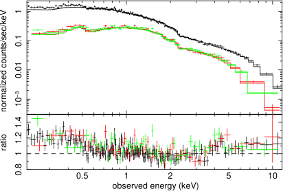
Figure 1.— XMM-Newton EPIC spectra of RBS 1055 in the observed frame. The spectra are fitted with a single power law (1PL) to data in the 1–12 keV range. At energies below 0.5 keV a soft excess is visible. A fluorescent 6.4 keV Fe K$\alpha$ line will be shifted to 4.4 keV at $z=0.450$.

Leaving the line energy as a free parameter slightly improves the fit ($\chi^{2}$/d.o.f. = 1264/1246; henceforth called the “2PLG2” model). We find $E_{\rm Fe,rest}=6.25\pm 0.22$ keV and $\sigma_{\rm Fe,rest}=0.49^{+0.24}_{-0.18}$ keV. Using the response matrix, we compute an instrumental energy resolution of FWHM${}_{\rm resol}\sim 160$ eV at the line energy. For all objects we will only consider a line to be significantly resolved if the line is resolved at the 95% (2$\sigma$) confidence level. Since a fit with an unresolved component (Gaussian line profile with a line centroid fixed at 6.4 keV and width $\sigma=0.001$ keV) results in a worse fit ($\chi^{2}$/d.o.f. = 1277/1247) and the lower limit 95% confidence errors of the measured $\sigma_{\rm Fe,rest}$ does not include $\sigma=0.001$ keV, we conclude that we have detected a resolved, neutral Fe K$\alpha$ line with EW$=0.14^{+0.14}_{-0.10}$ keV (3$\sigma$ uncertainties) in the spectrum of RBS 1055. We exclude the presence of an additional, unresolved component: we add a second narrow Gaussian with energy centroid fixed at 6.4 keV (rest frame) and $\sigma$ fixed at 1 eV, but this yields no improvement to the fit.

The freely fitted line energy of $E=6.25$ keV and the broad shape could potentially be caused by the presence of a Compton shoulder to the 6.4 keV Fe line. If so, we expect a Compton shoulder intensity of 20%–40% of the central Fe line, with a centroid energy of $\sim$6.3 keV (Matt 2002). Fixing the line energy of the primary Gaussian profile to 6.4 keV and including an additional Gaussian profile at a fixed energy of $E=6.3$ keV with an intensity of 30% of the primary Gaussian and a $\sigma=0.07$ keV (Bianchi et al. 2002) does not improve the fit. Leaving the line intensity as a free parameter causes its intensity to tend to zero and making the primary Gaussian the only significant source for modeling the Fe line.

We then tried to model the observed Fe line profile using a laor component (accretion disk around a Kerr black hole; Laor 1991), with an emissivity index fixed to 3, inclination to 30$\arcdeg$, and the outer radius to 400 gravitational radii ($r_{\rm g}=GM_{\rm BH}/c^{2}$). We achieved a fit virtually identical to that using a single Gaussian emission line (see above). The inner radius of emission is 16${}^{+16}_{-7}$ $r_{\rm g}$, i.e, poorly constrained due to the weakness of the line. Similar results are found for the high S/N spectra for RBS 320 and RBS 1124, and this model is thus not discussed further.

For RBS 1055, 320, and 1124, we determined the 90% confidence level upper limits of the equivalent width of a relativistically broadened Fe line in addition to a narrow profile by first modeling the Fe line with a Gaussian component (width $\sigma$ fixed to 1 eV) and then adding a laor component, leaving only the normalization of the laor component as a free parameter ($R_{\rm in}=1.235$ $r_{\rm g}$, $R_{\rm in}=400$ $r_{\rm g}$, and emissivity index 3). The resulting upper limits are discussed in Section 9.3.

To test if the soft excess and the broad Fe K$\alpha$ line can be modeled in a self-consistent manner, we employed the ionized reflection model reflion. We use a model of the form (kdblur*reflion)+zpo (Ross & Fabian 2005). Given the limited S/N of our spectra, some model parameters have to be fixed: we constrain the inclination to be 30$\arcdeg$, the outer radius of the reflecting disk to 400 gravitational radii, the emissivity index $q$ to 3, and the photon index of the reflected power law equal to that of the illuminating power law. Two almost identical $\chi^{2}$-fit minima are found (the reduced $\chi^{2}$ values are very similar): one fit (REFL1) is driven by both the soft excess and the Fe line and results in a low value of the ionization parameter; the second (REFL2) is driven by the shape of the soft excess and results in a high value of the ionization parameter.

For REFL1, the best-fit ($\chi^{2}$/d.o.f. = 1272/1247) yields an Fe abundance consistent with solar (Fe/solar $=1.4^{+0.7}_{-0.6}$), an inner radius of $R_{\rm in}=16.0^{+16.7}_{-11.4}$ $r_{\rm g}$, and the lowest possible value of the ionization parameter, $\xi_{\rm disk}=30^{+4}_{-0*}$ erg cm s^-1 (best-fit value pegged at hard limit of model); $\Gamma=1.77\pm 0.01$. The fraction of the reflected component to the total 0.2–12 keV output is 9%. The low ionization parameter models the Fe line well, but also causes relatively sharp line features in the soft excess model. Although a higher intensity of the reflected component would still be in agreement with the modeling of the observed Fe line, it would also increase the sharp line features in the soft excess which are not present in the data. Therefore, the best-fit is an attempt to explain both features simultaneously.

In the best-fit to REFL2, the fit ($\chi^{2}$/d.o.f. = 1268/1247) finds Fe/solar $=0.2^{+0.2}_{-0.1*}$, an inner radius of $R_{\rm in}<6.3$ $r_{\rm g}$, and $\xi_{\rm disk}=1500^{+700}_{-600}$ erg cm s^-1; $\Gamma=1.60^{+0.07}_{-0.09}$. The reflection model comprises 34% of the total 0.2–12 keV output and the parameters are driven to describe the smooth soft excess in the data up to 3 keV. This reflection component has only a very minor contribution to the high energies. Due to the high ionization parameter, the Fe K$\alpha$ line contribution is very broad, smeared out, and the line intensity too low. A higher Fe abundance is needed to improve the modeling of the Fe K line profile. However, this would cause a change in the shape of the soft excess around 0.7–0.9 keV in the rest frame, the energy range associated with Fe L emission, because the Fe K and Fe L line intensities are connected. Consequently, this model is also a compromise between accounting for the soft excess and representing the Fe line. Ignoring the energies around the Fe line still results in two equally good fit minima except that both are now found with the lowest Fe abundances possible.

Leaving the emissivity index $q$ free to vary in both models leads to a somewhat unconstrained emissivity index and improves the fit only marginally. We keep the values of the emissivity index frozen at 3 unless a free index results in improving the fit significantly (see Table 5). These values may not necessarily be representative of the physical/intrinsic emissivity indices, but such values are required to yield a soft excess with a smooth shape and thus achieve a good fit to the data.

The blurred reflection model can only successfully model Fe lines that originate in close proximity to the supermassive black hole and are relativistically broadened features. Therefore, we consider an additional narrow Fe line component with $E$ fixed at 6.4 keV and $\sigma$ fixed at 0.001 keV to model emission from gas located at large distances from the central region. This yields REFL1G and REFL2G, which differ from REFL1 and REFL2, respectively, by the addition of the narrow Gaussian line component. The residuals around 6.4 keV (rest frame) are better modeled in both cases (up to $\Delta\chi^{2}=-6$; Table 5), and we consider REFL2G to be the best-fit model for this spectrum.

Table 4Spectral Power-Law Fits for RBS 1055, RBS 320, RBS 1124, and RBS 1883

Model	$\Gamma$	$E_{\rm Fe,rest}$	$\sigma_{\rm Fe,rest}$	EWFe,rest	$\chi^{2}$/d.o.f.
		(keV)	(eV)	(eV)
RBS 1055
1PL	1.79$\pm$0.01	–	–	–	1413/1251
2PL	1.37${}^{+0.20}_{-0.37}$ & 2.12${}^{+0.31}_{-0.17}$	–	–	–	1281/1249
2PLG	1.13${}^{+0.38}_{-0.11}$ & 1.98${}^{+0.01}_{-0.10}$	!6.4!	480${}^{+220}_{-180}$	$140^{+70}_{-50}$	1266/1247
2PLG2	1.07${}^{+0.39}_{-0.09}$ & 1.97${}^{+0.25}_{-0.09}$	$6.25\pm 0.22$	490${}^{+240}_{-180}$	$140^{+60}_{-50}$	1264/1246
RBS 320
1PL	2.69$\pm$0.01	–	–	–	1615/810
2PL	1.91${}^{+0.11}_{-0.12}$ & 3.31${}^{+0.13}_{-0.11}$	–	–	–	934/808
2PLG	1.95$\pm$0.10 & 3.32${}^{+0.11}_{-0.12}$	!6.4!	270${}^{+420}_{-200}$	120${}^{+110}_{-70}$	924/806
2PLG2	1.95${}^{+0.11}_{-0.10}$ & 3.32$\pm$0.12	6.47${}^{+0.21}_{-0.22}$	260${}^{+370}_{-200}$	130${}^{+90}_{-80}$	924/805
RBS 1124
1PL	1.96$\pm$0.01	–	–	–	1660/1293
2PL	$1.13\pm 0.04$ & $2.19\pm 0.03$	–	–	–	1525/1291
2PLG	$1.15\pm 0.05$ & $2.19\pm 0.04$	!6.4!	180${}^{+320}_{-120}$	70${}^{+60}_{-40}$	1516/1289
2PLG2	$1.15\pm 0.05$ & $2.19\pm 0.04$	$6.49\pm 0.14$	140${}^{+240}_{-140}$	70${}^{+60}_{-40}$	1515/1288
1PL	1.79$\pm$0.01	–	–	–	1122/926
2PL	1.58${}^{+0.08}_{-0.10}$ & 2.74${}^{+0.29}_{-0.30}$	–	–	–	958/924
2PLG	$1.58\pm 0.08$ & 2.68${}^{+0.40}_{-0.23}$	!6.40!	120${}^{+140}_{-120}$	51${}^{+34}_{-26}$	942/922
2PLG2	1.60${}^{+0.06}_{-0.10}$ & 2.74${}^{+0.33}_{-0.28}$	6.40${}^{+0.08}_{-0.12}$	120${}^{+150}_{-120}$	52${}^{+34}_{-29}$	942/921
RBS 1883
1PL	2.9$\pm$0.1	–	–	–	180/86
2PL	1.7$\pm$0.3 & 3.9${}^{+0.5}_{-0.4}$	–	–	–	119/84

Note. — Models (explanation of models according to the Xspec notation): 1PL – single power law (phabs(zpo)), 2PL – two power laws, one fitting the soft energy range, the other, the hard energy range (phabs(zpo1+zpo2)), 2PLG – two power laws including a Gaussian component with a line energy fixed to 6.4 keV in the rest frame (phabs(zpo1+zpo2+zgauss)), 2PLG2 – same as 2PLG but line energy is allowed to vary. Frozen parameters are in exclamation marks. Energies and equivalent widths are given in the quasar rest frame. Uncertainties are computed for the 90% confidence interval. For RBS 1124 we show the results of the 0.35–10 keV Suzaku data fits in italic font, while all 0.2–12 keV XMM-Newton-based fits are in roman font.

Table 5Results for REFL1G and REFL2G: Disk Reflection Plus a Narrow Fe Line component

$\chi^{2}$/d.o.f.	$\Gamma$	$q$	$R_{\rm in}$	$\xi$	Fe/Solar	$\Delta\chi^{2}$
			($r_{\rm g}$)	(erg cm s-1)		Fe Line
RBS 1055
1271/1246	1.77${}^{+0.02}_{-0.01}$	!3!	15.9${}^{+17.8}_{-10.5}$	30${}^{+4}_{-0*}$	1.4${}^{+0.5}_{-0.7}$	1
1262/1246	1.60${}^{+0.07}_{-0.09}$	!3!	2.6${}^{+2.5}_{-1.4*}$	1600${}^{+700}_{-600}$	0.2${}^{+0.2}_{-0.1*}$	6
RBS 320
933/804	2.65${}^{+0.08}_{-0.05}$	8.4${}^{+1.6*}_{-2.1}$	2.3${}^{+0.3}_{-0.4}$	110${}^{+150}_{-80*}$	0.1${}^{+0.2}_{-0*}$	7
971/804	2.39${}^{+0.02}_{-0.03}$	7.2${}^{+1.4}_{-0.9}$	1.9${}^{+0.6}_{-0.3}$	$1500\pm 200$	$0.3\pm 0.1$	10
RBS 1124
1541/1288	1.94${}^{+0.01}_{-0.02}$	!3!	3.1${}^{+2.5}_{-1.9*}$	30${}^{+8}_{-0*}$	3.5${}^{+2.5}_{-2.4}$	1
1514/1288	1.55${}^{+0.09}_{-0.14}$	!3!	7.2${}^{+2.8*}_{-4.4}$	9700${}^{+300*}_{-1600}$	2.8${}^{+3.9}_{-1.0}$	2
930/921	1.81${}^{+0.04}_{-0.03}$	!3!	1.2${}^{+1.7}_{-0*}$	40${}^{+34}_{-10*}$	1.7${}^{+0.9}_{-0.8}$	4
931/920	$1.17^{+0.10}_{-0.06}$	8.0${}^{+2.0*}_{-1.9}$	1.2${}^{+0.4}_{-0*}$	7000${}^{+3000*}_{-5000}$	3.3${}^{+2.3}_{-2.5}$	14

Note. — For explanation see Table 4. A lower/upper 90% confidence uncertainty marked with “*” symbolizes that the parameter pegged at the lower/upper hard limit of the model. All fits use frozen parameters of: inclination angle = 30$\arcdeg$, $R_{\rm out}=400$ $r_{\rm g}$, $E_{\rm Fe,rest}=6.4$ keV, and $\sigma_{\rm Fe,rest}=1$ eV.

We also try to incorporate two reflection components to account for reflection in different region: one very close to the central engine producing the smooth shape of the soft excess, the other far away to produce the narrow Fe line. However, the moderate quality of the XMM-Newton data for all objects does not allow us to constrain crucial parameters such as the break radius (radius of inner and outer reflection) and ionization parameter of the inner disk.

The RGS data of RBS 1055, as well as for all other high S/N RBS-QSOs, are well fitted with a single power law ($\chi^{2}$/d.o.f. = 207/240). No significant absorption or emission features are visible based on only the RGS data of RBS 1055. The upper limits to the absolute values of equivalent widths (90% confidence level) of typical prominent narrow emission and absorption lines such as O VII, O VIII, Ne IX and Ne X are as high as $\sim 8$ eV. Both disk reflection scenarios fit equally well the RGS data.

Considering the best-fit model for RBS 1055 (REFL2G), we give the intrinsic (corrected for Galactic absorption) 0.5–2 keV and the 2–10 keV fluxes of the object as well as the corresponding intrinsic luminosities for all objects in Table 3.

5.2. X-ray Spectra of RBS 320

For the analysis of the RBS 320 data (and the remaining RBS objects), we follow the same approach as described in detail for RBS 1055. We will only summarize the most important findings. As for RBS 1055, we also find that a 2PL model is required to characterize the overall shape of the RBS 320 data appropriately ($\chi^{2}$/d.o.f. = 934/808) although positive residuals are still present at 6–7 keV (rest frame) where the Fe K$\alpha$ line is expected (see Figure 2).

A PLBB model ($k_{\rm B}T=0.09\pm 0.01$ keV, $\Gamma=2.42\pm 0.02$) cannot fit the data well ($\chi^{2}$/d.o.f. = 1099/808). The best-fit partial covering model incorporating absorption by a gas with a column density of $N_{\rm H}\sim 2\times 10^{23}$ cm^-2 and a covering fraction of $\sim$60% fails to properly model the data ($\chi^{2}$/d.o.f. = 1071/808). A moderately-good fit is obtained for full-covering absorption model with ionized material ($\chi^{2}$/d.o.f. = 935/806). However, this fit finds a very high ionization value (log $(\xi$/(erg cm s^-1))$=6$, lower 90% limit: log $(\xi$/(erg cm s^-1))$=3.3$) and an unconstrained $N_{\rm H,warm}$ value. Ionization parameters log $(\xi$/(erg cm s^-1))$>4$ do not change the overall shape of the X-ray spectrum; they only include narrow H-like absorption lines which are not seen in the data. Therefore, we also exclude for RBS 320 the presence of a warm absorber. An edge component with energy fixed at 7.1 keV does not improve the fit of the 2PL model ($\chi^{2}$/d.o.f. = 934/807, 90$\%$ confidence upper limit on $\tau=0.19$). Consequently, also in the case of RBS 320 we conclude that an Fe K$\alpha$ emission line is detected.

Adding a Gaussian component to the 2PL model results in an improved fit (2PLG, $\chi^{2}$/d.o.f. = 924/806, Table 4) and yields $\sigma_{\rm Fe,rest}=0.27^{+0.42}_{-0.20}$ keV for an Fe K$\alpha$ line with energy centroid fixed at $E=6.4$ keV. The line is detected at more than 3$\sigma$ confidence. Fixing $\sigma=0.001$ keV results in a fit with $\Delta\chi^{2}=+3$. Following our general guideline for the detection of a resolved line, the line is not resolved. Leaving the line energy as a free parameter (2PLG2) does not change the fit. A Compton shoulder to the Fe line is not consistent with the data.

Applying REFL1 with an emissivity index fixed to 3 results in a moderately good representation of the data ($\chi^{2}$/d.o.f. = 1032/806) when the lowest possible ionization parameter is used ($\xi=30^{+3}_{-0*}$ erg cm s^-1). The fit significantly improves when thawing the emissivity index ($q=8^{+2*}_{-2}$, $\chi^{2}$/d.o.f. = 940/805). At $q=3$ the soft excess is still modeled with some structure not seen in the data and peaks at around 0.6 keV (rest frame; O VII), while much higher $q$ values again result in a much more smooth soft excess without any structure and shift its peak to below 0.4 keV which is consistent with the data. The Fe K$\alpha$ line is too weak and too broad in this model. The same trend can be found when we keep $q=3$ fixed and leave the outer disk radius as a free parameter. In this case, the best-fit ($\chi^{2}$/d.o.f. = 943/805) results in an outer disk radius of only $R_{\rm out}=4.1^{+0.4}_{-1.2}$ $r_{\rm g}$ to model the soft excess as smooth as possible. However, we decide to fix the outer radius at $R_{\rm out}=400$ $r_{\rm g}$ and leave $q$ as a free parameter. The reflection component represents 21% of the total 0.2–12 keV output.

As in the case for RBS 1055, we find a second best-fit model (REFL2) with a local fit minimum at an ionization parameter of $\xi=1500^{+200}_{-300}$ erg cm s^-1 and $q$ as a free parameter, where the reflection component represents 56% of the total 0.2–12 keV output. However, this fit minimum is worse ($\chi^{2}$/d.o.f. = 981/805) than the fit with the low ionization parameter (REFL1) because it contains a smaller contribution at hard energies and leaves positive residuals around 6–7 keV.

Applying REFL1G and REFL2G by adding a narrow Gaussian component with energy centroid fixed at $E=6.4$ keV and with the line width fixed at $\sigma=0.001$ keV improves each fit further (Table 5). Leaving the line energy as a free parameter only marginally improves the fit. The line has EW$=0.05^{+0.04}_{-0.03}$ keV in REFL1G (EW$=0.06^{+0.04}_{-0.03}$ keV for REFL2G).

The power-law fit of the RGS data ($\chi^{2}$/d.o.f. = 220/251) improves when we add two Gaussian line profiles in emission at rest-frame energies of $E=1.04\pm 0.01$ keV and $E=1.24^{+0.02}_{-0.04}$ keV ($\chi^{2}$/d.o.f. = 208/246). Both lines are unresolved and have rest frame equivalent widths of EW$=10^{+2}_{-7}$ eV and EW$=7^{+7}_{-5}$ eV, respectively. Because the fit improves by $\Delta\chi^{2}=-8$ and –5, respectively, the lines are detected at the 2–3$\sigma$ confidence level. In the case of the first line, the energy centroid is not far from the expected line energy for Ne X, 1.022 keV, but thanks to the resolution of the RGS, this energy is ruled out at more than 95$\%$ confidence. The origins of these tentatively detected lines thus remain unclear. Adding Gaussian components in emission or absorption at the rest-frame energies of expected H or He-like metals result in upper limits to the absolute value of equivalent widths up to 2 eV. Both disk reflection scenarios fit the RGS data equally well.

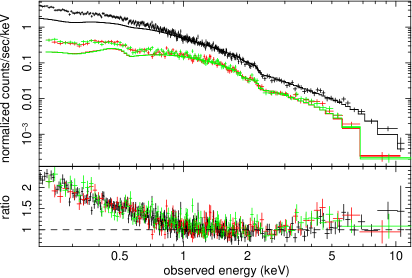
Figure 2.— XMM-Newton EPIC spectra of RBS 320 in the observed frame. The 1–12 keV energy range is fitted with a 1PL model. The 6.4 keV Fe K$\alpha$ line will be shifted to 4.3 keV at the object’s redshift of $z=0.495$.

5.3. X-ray Spectra of RBS 1124

A 2PL model again represented the data better ($\chi^{2}$/d.o.f. = 1525/1291) than a 1PL model ($\chi^{2}$/d.o.f. = 1660/1293; see Table 4 and Figure 3). The PLBB model does not provide a better fit ($k_{\rm B}T=0.14\pm 0.01$ keV, $\Gamma=1.88\pm 0.02$, $\chi^{2}$/d.o.f. = 1580/1291). A partial covering model with a column density of $N_{\rm H}\sim 4\times 10^{23}$ cm^-2 and a covering fraction of $\sim$21% describes the data very well ($\chi^{2}$/d.o.f. = 1515/1291). A full-covering and partial-covering absorption model with ionized material can be excluded because they both require very high column densities and ionization parameters ($N_{\rm H}\sim 1\times 10^{24}$ cm^-2, log $(\xi$/(erg cm s^-1))$=5$; see explanation for RBS 320). Furthermore, we exclude an Fe edge component at 7.1 keV (rest frame) to account for the positive residuals around 6 keV (rest frame) in 2PL model (90$\%$ confidence upper limit on $\tau=0.02$).

Adding a Gaussian component to a 2PL model improved the fit further by $\Delta\chi^{2}=-9$ (2PLG, $\chi^{2}$/d.o.f. = 1516/1289). Consequently, the line is detected at the 3$\sigma$ confidence level. Fixing the width of the line to $\sigma=0.001$ keV yields $\chi^{2}$/d.o.f. = 1521/1290. The line is resolved since the lower 2$\sigma$ limit of the line width is not consistent with the expected value for an unresolved line. Leaving the line energy as a free parameter (2PLG2) only improves the fit marginally ($\Delta\chi^{2}=-1$).

The self-consistent disk reflection model (REFL2) results in a very good fit of the data (emissivity index fixed to 3, $\chi^{2}$/d.o.f. = 1516/1289). We find an extremely high ionization parameter of $\xi=9000^{+1000*}_{-2000}$ erg cm s^-1 and almost solar abundances. The reflection component accounts for 75% of the total 0.2–12 keV output. With the best-fit parameters of this model, the shape of the reflection component is very similar to a simple power-law fit except that it models a very broad and smeared out Fe line.

As for RBS 1055 and RBS 320, a second stable local $\chi^{2}$-minimum is found for a fit with low $\xi$ values (REFL1, $\chi^{2}$/d.o.f. = 1542/1289). REFL1 introduces discrete line features to model the soft excess and the Fe line. Since RBS 1124’s soft excess is again very smooth, the reflection component can only account for 6% of the total 0.2–12 keV output in order to avoid introducing significant structure to the soft excess. Furthermore, REFL1 predicts a slope which is too steep at high energies compared to the data.

Thawing the emissivity index $q$ does not affect the quality of REFL1 and REFL2 significantly and $q$ is found to be unconstrained in both fit models. Therefore, we decide to leave it fixed to $q=3$. Considering an additional narrow Gaussian line profile (REFL1G and REFL2G) with a fixed rest-frame energy of 6.4 keV improves both disk reflection fit models marginally. The line has an EW$=0.03^{+0.03}_{-0.02}$ keV in REFL1G and REFL2G.

After fitting the RGS data with a single power-law model ($\chi^{2}$/d.o.f. = 349/349), no narrow striking spectral features are visible (upper limits to absolute values of EWs on prominent narrow emission and absorption lines are up to EW $\sim$ 5 eV). The RGS data are again equally well fitted by both reflection scenarios.

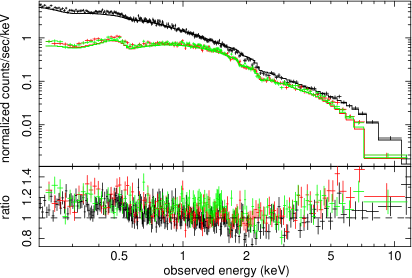
Figure 3.— XMM-Newton EPIC spectra of RBS 1124 in observer frame. A 1PL is fitted to the 1–12 keV energy band. The 6.4 keV Fe K$\alpha$ line will be shifted to 5.3 keV at the object’s redshift of $z=0.209$.

5.4. Joint Fit Analysis of XMM-Newton and Suzaku Spectra

RBS 1124 was also observed with Suzaku on April 14–16, 2007 (ObsID 702114010) for a duration of 138 ks (before screening for Earth occultation, etc.). The analysis and results of this observation are published in Miniutti et al. (2010). We include in this paper joint spectral fitting of the XMM-Newton and Suzaku spectra to achieve better constraints on spectral fit parameters for the Fe line compared to XMM-Newton alone. In addition, the two observations of RBS 1124 gives us the opportunity to study spectral variability in one of the most luminous radio-quiet QSOs on a 13 month time scale and with comparable S/N spectra.

5.4.1 Suzaku RBS 1124 Data Reduction

The data were obtained with the X-ray imaging CCDs (XIS; Koyama et al. 2007) on board Suzaku, which consist of two front-illuminated (FI) CCD and one back-illuminated (BI) CCD (XIS2 was not used), as well as the non-imaging hard X-ray detector (HXD; Takahashi et al. 2007). RBS 1124 was placed at the “HXD nominal” position. The XIS and HXD data are processed with Suzaku pipeline processing version 2.0.6.13. The analysis uses the HEADAS version 6.6.1. software. The XIS data reduction follow the guidelines provided in the Suzaku Data Reduction Guide. As per a notice for a calibration database update the task xispi is run on the unfiltered events again. The events are filtered using standard extraction criteria (e.g., avoiding the South Atlantic Anomaly, low Earth elevation angles, etc.). The XIS good integration time is 86 ks per CCD. We extract for each of the three XIS CCDs the source events by choosing a region 3$\arcmin$ in radius, the background events by four regions 1$\farcm$5 in radius, and the ⁵⁵Fe calibration source events. RBS 1124 is detected with a net count rate of 0.29 ct s^-1 in the XIS FI and 0.39 ct s^-1 in the XIS BI. The response (RMF) and auxiliary (ARF) file are produced by using the tasks xisrmfgen and xissimarfgen. The data for both XIS FI detectors are co-added to form a single spectrum using mathpha, addrmf, and addarf. Finally the data are grouped to at least 20 counts per bin.

The Mn I K$\alpha_{1}$ and K$\alpha_{2}$ lines in the calibration spectrum are fitted by two Gaussian components, where the K$\alpha_{2}$ Gaussian component has half the intensity of K$\alpha_{1}$. The nominal rest-frame energies of Mn I K$\alpha_{1}$ and K$\alpha_{2}$ are 5.899 keV and 5.888 keV, respectively, with an expected intensity ratio of 2:1. The observed K$\alpha_{1}$ line peaks at $E=5.897\pm 0.001$ keV for the added XIS FI and $E=5.897\pm 0.002$ keV for the XIS BI with an upper limit up to $\sigma=16$ eV (co-added FI and BI). The FWHM energy resolution is 149 eV for the present observation.

The 12–76 keV HXD/PIN data are also reduced following the Suzaku guidelines. As in Miniutti et al. (2010), we find that an extrapolation of the XIS spectral fit to higher energies does not agree with the PIN data. Walton et al. (2010) explain similar Suzaku spectra (e.g., 1H 0419-577) with two reflection disk models: one (with kdblur) modeling the effects of strong gravity in the innermost region of the disk, the other (without kdblur) accounting for reflection at far distances. Although modeling the data better than a 2PL fit, the proposed models, including splitting the disk into an inner and outer region, still leave strong positive residuals at energies below 20 keV (observed frame). Since the origin of the observed steep excess in the PIN data below 20 keV (observed frame) still remains unclear (likely an additional variable hard X-ray source in the HXD/PIN field of view or instrumental issues), we decide not to use the PIN data.

5.4.2 Suzaku X-ray Spectra of RBS 1124

Miniutti et al. (2010) focus on fitting the Suzaku RBS 1124 data with the self-consistent disk reflection model reflion and a partially covering model. We briefly summarize our fit results which also includes detailed power-law fits on the Suzaku 0.3–10 keV spectrum of RBS 1124. We fit the spectrum over 0.3–9 keV for the XIS BI and 0.4–11.5 keV for the co-added XIS FI. Furthermore, we ignored energies in the range 1.75–1.90 keV to avoid calibration uncertainties associated with the instrumental Si K-edge. Leaving the normalization difference between the XIS FI and BI as a free parameter to account for instrumental cross-calibration improves all fits (e.g., 1PL by $\Delta\chi^{2}=-15$). We find a normalization constant between both instrument types of approximately 0.98.

A 2PL model fits also the Suzaku data better than a 1PL model (Table 4, $\chi^{2}$/d.o.f. = 958/924 versus $\chi^{2}$/d.o.f. = 1122/926). The PLBB model is a very good representation of the data ($\chi^{2}$/d.o.f. = 947/924, $\Gamma=1.72\pm 0.02$, $k_{\rm B}T=0.14\pm 0.01$ keV). A partial-covering absorption model with neutral material does not explain the data well ($\chi^{2}$/d.o.f. = 968/924, $\Gamma=1.94\pm 0.03$, $N_{\rm H}\sim 2\times 10^{23}$ cm^-2, and a covering fraction of $\sim$30%). There are no obvious narrow discrete absorption features seen that would suggest the presence of an ionized absorber as well. We return to the 2PL fit and add a Gaussian line profile. The 2PLG model improves the fit ($\chi^{2}$/d.o.f. = 942/921) and an Fe line is detected at greater than the 4$\sigma$ confidence level. Fixing the line width to $\sigma=0.001$ keV results in $\chi^{2}$/d.o.f.= 944/922. The line is not resolved.

REFL1, the self-consistent disk reflection model without an additional narrow Fe line, is a very good representation of the data ($\chi^{2}$/d.o.f. = 934/921, emissivity index frozen) when an ionization parameter of $\xi_{\rm disk}=38^{+25}_{-8*}$ erg cm s^-1 is used. The reflection component accounts for 13% of the total 0.2–12 keV output. We also find in the Suzaku data a second fit minimum incorporating a high ionization parameter (REFL2, $\chi^{2}$/d.o.f. = 967/922, $\xi_{\rm disk}=2200^{+1200}_{-800}$ erg cm s^-1 and keeping the emissivity index fixed to 3). REFL2 significantly improves ($\Delta\chi^{2}$ = -22) when the emissivity index is allowed to vary ($q=10^{+0*}_{-3}$, $\xi_{\rm disk}=6700^{+3300*}_{-2800}$ erg cm s^-1). This reflection model makes up 54% of the total 0.2–12 keV output.

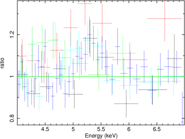
Figure 4.— To illustrate the Fe K$\alpha$ fluorescence line in RBS 1124 we show the data/model residuals for a 2PL model fit, i.e., without the Fe line modeled, to the XMM-Newton EPIC (black – pn, red – MOS1, and green – MOS2) and Suzaku (dark blue – XIS FI, light blue – XIS BI) spectra.

We then added a narrow Fe line to the reflection models (REFL1G and REFL2G) and find improvements to the fit compared to REFL1 and REFL2, respectively (Table 5). Model REFL2G improves by $\Delta\chi^{2}$ = -24 when the emissivity index is left as a free parameter. Our fit results for model REFL1G are consistent with the values given in Miniutti et al. (2010) considering the uncertainties. Based on model REFL1G we derive intrinsic $f_{\rm 0.5-2}=3.0\times 10^{-12}$ erg cm^-2 s^-1 ($f_{\rm 2-10}=4.8\times 10^{-12}$ erg cm^-2 s^-1) and a corresponding $L_{\rm 0.5-2}=3.8\times 10^{44}$ erg s^-1 ($L_{\rm 2-10}=5.8\times 10^{44}$ erg s^-1).

The total 0.5–2 keV flux and total 2–10 keV flux both increased between the Suzaku and XMM-Newton observation, by roughly 60% and 35%, respectively. In the context of the 2PL model, there is evidence for both the 1 keV normalization and photon index of both power-law components (soft and hard) to vary between the observations. The soft excess contribution according to a phenomenological blackbody model (computing the contribution of the blackbody model to the total 0.5–2 keV flux) has decreased from ($9\pm 1$)% in the Suzaku observation to ($5\pm 1$)% in the XMM-Newton observation 13 months later. Because the soft excess is observed to vary, an origin in a very extended or distant region (greater than 13 light months from the central X-ray source) is ruled out. The detailed relation between the origins and interactions of the soft excess and the hard power law for RBS 1124 remain unclear. However, the parameters for the Fe line profile do not vary between the two observations (line parameters are consistent within the 1$\sigma$ uncertainties), and so we can do a joint fit to achieve better constraints on the Fe line.

5.4.3 Fe Line Constraints Through a Joint Fit

For the joint fit we use the same energy ranges that we used for the single spectral fits. We apply the 2PLG model to the data. For the Suzaku data we keep the BI/FI normalization constant frozen at $c=0.98$. Tying the slopes of the soft and hard power laws for both observation and only using different normalizations yield a very bad fit with very significant residuals. Consequently, we leave both the 1 keV normalization and the photon indices of the soft and hard power law free to vary between the Suzaku and XMM-Newton observations. Allowing the line width and the line energy to vary between both observations does not improve the fit further.

We derive an Fe line width of $\sigma_{\rm Fe,rest}=0.14^{+0.10}_{-0.09}$ keV from the joint fit (Figure 4). If we omit the line component, the fit worsens by $\Delta$$\chi^{2}=24$, while fixing the line width to 1 eV worsens the fit by $\Delta$$\chi^{2}=8$. Consequently, using a joint fit to both observations, we detect the Fe line with a much higher significance than in the individual observations. The line is resolved and has an intensity of $I=(5.2\pm 2.1)\times 10^{-6}$ ph cm^-2 s^-1.

5.5. X-ray Spectra of RBS 1883

The observation of RBS 1883 suffers heavily from very high background count rates throughout almost the entire observation. Although the low number of counts does not allow us to study RBS 1883 as detailed as the other RBS QSOs presented in this paper, a 2PL model fits the data much better than a 1PL ($\chi^{2}$/d.o.f. = 180/86 versus 119/84; see Table 4 and Figure 5). A PLBB model results in a fair fit of the data ($k_{\rm B}T=0.13\pm 0.01$; $\chi^{2}$/d.o.f. = 124/84).

A partial covering model improves the fit ($\chi^{2}$/d.o.f. = 113/84) by finding a very high covering fraction of (82$\pm$6)% and $N_{\rm H,cov}=(1.4^{+0.6}_{-0.4})\times 10^{23}$ cm^-2. The S/N of the data does not allow us to test for a warm absorber in RBS 1883; the ionization parameter and $N_{\rm H,warm}$ stay unconstrained. For the same reason we are not able to apply a reflecting disk model to the data.

Although no emission line features, e.g., an Fe K$\alpha$ line, are visible in the spectra, we included a Gaussian component fixed to an energy of 6.4 keV (rest frame) to give upper limits on the Fe K$\alpha$ emission line. For an unresolved Fe line (width $\sigma=0.001$ keV), we find an 90% confidence level upper limit on the EW$<0.66$ keV (EW$<0.84$ keV for a resolved Fe line with $\sigma$ fixed to 0.4 keV).

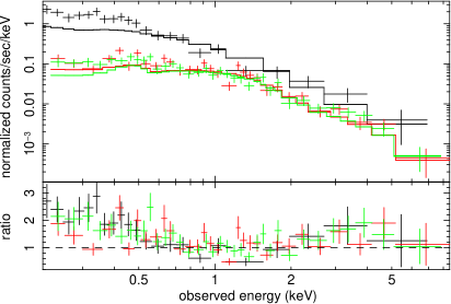
Figure 5.— XMM-Newton EPIC spectra of $z=0.545$ RBS 1883 in observer frame. A 1PL is fitted to the 0.5–12 keV energy band.

6. Optical-to-X-ray spectral Indices

The optical monitor (OM) onboard XMM-Newton provides UV photometric data for all objects taken simultaneously with the X-ray data and therefore enables us to calculate optical-to-X-ray spectral energy distributions ($\alpha_{\rm ox}$) without the uncertainties introduced by source variability. The OM source lists produced by the XMM-SAS pipeline contain calibrated source magnitudes in the AB system that are also corrected for the long term degradation of the OM. In addition, we de-redden the UV data using the maps by Schlegel el al. (1998) and the wavelength dependencies by Cardelli et al. (1989).

The four OM observations of the RBS-QSOs were taken with different filter combinations. To derive the $k$-corrected rest-frame luminosity densities at 2500 Å, we use the mean UV continuum slope $\alpha_{\rm uv}=-0.44$ (frequency index) of the SDSS QSO spectra (Vanden Berk et al. 2001). If we have more than one magnitude measurement for an individual object, we select the filter observation which is less affected by a strong UV emission line. The only OM detection of RBS 320 in filter UVM2 coincides with the C IV line in the object and the derived values should be considered with care. The rest-frame luminosity densities at 2 keV is computed from the 0.5–2 keV rest-frame luminosities given in Table 3 and the photon indices measured in the same energy range (Table 8). Considering the redshift of our objects, the 2 keV rest-frame luminosity density will be redshifted into the 0.5–2 keV band. The measured magnitudes and the derived quantities are listed in Table 6.

Table 6Magnitudes, Rest-frame Luminosity Densities, $\alpha_{\rm ox}$

Object	AB Magnitude/	log$l_{2500{\rm\,\AA}}$	log$l_{\rm 2\,keV}$	$\alpha_{\rm ox}$
Name	Filter
RBS 1055	18.18$\pm$0.02/UVW1∗	30.11	27.41	1.04
	17.26$\pm$0.03/UVM2
RBS 320	15.44$\pm$0.01/UVM2	31.25	27.15	1.26
RBS 1124	16.44$\pm$0.01/UVW1	30.07	26.94	1.20
RBS 1883	16.33$\pm$0.01/UVW1
	16.29$\pm$0.02/UVW2∗	30.98	26.91	1.57

The derived $\alpha_{\rm ox}$ values cover the same range that is found by Grupe et al. (2010) in a sample of soft X-ray selected AGN drawn from the RASS survey and observed with Swift. They also observed RBS 1124 and find an $\alpha_{\rm ox}=1.23$. Considering this Swift sample, RBS 1055 yields an $\alpha_{\rm ox}$ value on the low edge of the distribution. Our values are also consistent with the sample by Anderson et al. (2007, 2003) who spectroscopically identified 7000 RASS AGN from the Sloan Digital Sky Survey (data release 5).

7. Long-term Flux Variability of the RBS-QSOs

Since all the studied objects in this work have been observed with ROSAT and XMM-Newton separated by almost two decades, both measurements allow a crude long-term flux variability study. The RBS contains the flux-brightest (with some spatial restrictions) objects from the RASS which was observed in 1990/1991 during the first half year of the ROSAT mission. RBS 1124 has also been observed by the XMM-Newton Slew Survey, Suzaku, and Swift (see Miniutti et al. 2010). RBS 320 was observed four years after the XMM-Newton observation with Swift on 2008 November 7 (target name: QSO B0226-4110; target ID: 37516). We used the online Swift XRT data reduction pipeline (Evans et al. 2009) to extract a $\sim$13 ks spectrum. Binning the data to 20 counts per bin, the low S/N ($\sim$1000 counts) Swift spectrum requires only a single power-law fit ($\Gamma=2.58\pm 0.09$, $\chi^{2}$/d.o.f. = 41/42) with no intrinsic absorption. This is consistent with the 1PL fit of the XMM-Newton data considering the uncertainties.

Figure 6.— Intrinsic (Galactic-absorption corrected) flux vs. time for the studied RBS-QSOs. The symbols represent measurements from different missions: triangle – ROSAT, square – XMM-Newton, diamond – Swift, asterisk – XMM-Newton Slew Survey, and cross – Suzaku.

The 0.5–2 keV ROSAT fluxes are taken from the RBS catalog (Schwope et al. 2000). They assumed a photon index of $\Gamma=2$ to compute count-to-energy conversion factor for the ROSAT PSPC detectors considering the Galactic column density toward the X-ray source. To keep possible flux changes due to the different flux computation methods between ROSAT (RBS) and the measurements from other missions as low as possible (flux differences up to 10%), we applied the RBS technique to all observations. Figure 6 shows all measured fluxes for the studied RBS-QSOs versus time. Except for the decrease and rise of RBS’s 1124 flux between 2006 November and 2008 May, all objects show only flux variability on a level of $\sim$5%–20% based on the few data points available.

8. Construction of an Average X-ray Spectrum

We decided to construct an average X-ray spectrum for the four sources studied here. First, the average spectrum may unveil a possible relativistic component of the Fe K$\alpha$ emission line in the most luminous radio-quiet RBS-QSOs due to the increase in S/N. Secondly, the average broadband spectral properties in these objects can be compared to the average broadband spectral properties obtained for high-redshift, low S/N spectra with very similar X-ray luminosities found routinely by the XMM-Newton and Chandra surveys (e.g., Mateos et al. 2010; Brusa et al. 2005). This will test if our most luminous radio-quiet RBS-QSO X-ray spectra, which allow us to determine their spectral properties directly, are the standard cases of luminous radio-quiet QSOs at high redshifts.

The averaging process follows Corral et al. (2008) with some differences. The original process was designed to average a large number of sources to improve the S/N, whereas here we are only averaging four sources. Therefore, the influences of individual sources on the average spectrum is considerably higher. We tested the source-to-source influence on the average spectrum by generating sets of average spectra, removing one source in each case. The results are robust, i.e., the derived properties vary within their 2$\sigma$ limits. In particular, removing RBS 1055, which has the broadest Fe line, does not change the properties of the averaged Fe line.

We are forced to exclude the pn data for RBS 1883 since, given the small number of counts at high energies in this case, it distorts the average spectrum shape at those energies. The main steps of the averaging process are as follows: We fit a 2PL model to each spectrum, instead of the simple absorbed power law as described in Corral et al. (2008), since, as we show above, this is a very good representation of the X-ray data for the whole sample. Then we obtain the incident spectrum for each source, i.e., the source spectrum before entering the detector, by using the previously obtained model and the Xspec command eufspec. Doing so, we derive the source spectra in flux units of keV cm^-2 s^-1 keV^-1. Next, we de-absorb each spectrum for the Galactic absorption at each source position and shift them to their rest frame. To combine the individual spectra, we rescale them by forcing the rest frame 2–5 keV flux to be the same for all objects. Finally, we rebin the spectra to a common energy grid in a range of 1–13 keV, ensuring that all bins contain at least 600 real counts, and average them by using a standard mean. Individual errors on the real spectra are propagated as Gaussian along the whole averaging process. The significances of the individual spectral features in the final average spectrum are quantified by using simulations. We simulate each source 100 times using its best-fit model and keeping the same spectral quality and flux as for the real source. We apply exactly the same averaging process to the simulated spectra as we do for the real spectra. From the 100 simulated spectra, we compute the confidence limits (1$\sigma$ and 2$\sigma$ confidence encompass 68% and 95% of the simulated values, respectively) and a simulated continuum, which account for the mixture of 2PL shapes. As already suggested by the individual X-ray spectra, the resulting average spectrum contains in comparison to a 2PL no spectral features except an Fe line which is detected above the 2$\sigma$ confidence limit. The Fe K bandpass is shown in Figure 7.

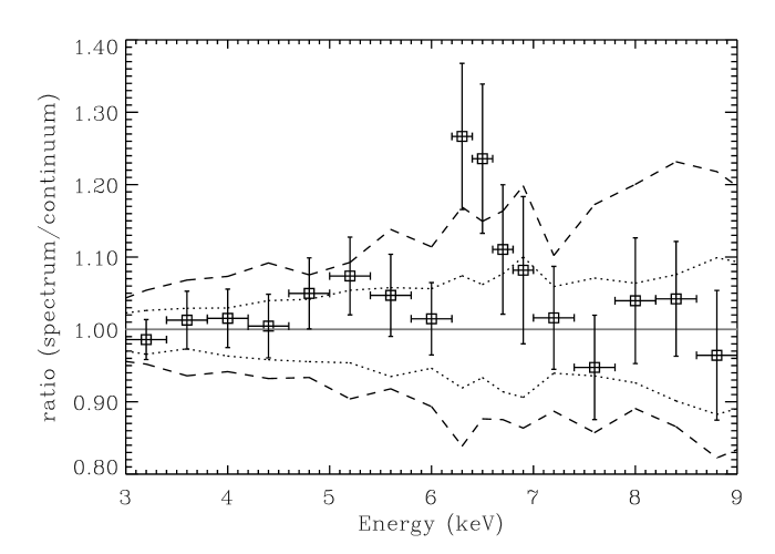
Figure 7.— Added XMM-Newton spectrum of RBS 1055, RBS 320, RBS 1124, and RBS 1883. The stack contains $\sim$35,000 counts in the shown 3–9 keV range. The squares represent the ratio between the flux of the stacked spectrum and the simulated continuum spectrum. The uncertainties of the bins of the stacked spectrum are shown as error bars. The dotted lines show the 1$\sigma$ confidence limits, while the dashed line represents the 2$\sigma$ confidence limits. The solid gray line at a ratio of one illustrates the continuum flux.

Following the analysis on individual objects, we first fit a 2PL to the 1–12 keV rest frame data. We achieve a good fit of $\chi^{2}$/d.o.f. = 22/19 ($\Gamma_{\rm soft}=3.4^{+0.7}_{-0.5}$, $\Gamma_{\rm hard}=1.7^{+0.1}_{-0.2}$). The remaining positive residuals can be well fitted by adding a Gaussian profile. The 2PLG model improves the fit to $\chi^{2}$/d.o.f. = 8/16 and yields $\Gamma_{\rm soft}=3.4^{+0.8}_{-0.6}$, $A_{\rm soft}=0.8^{+0.3}_{-0.2}$ ph cm^-2 s^-1 keV^-1 (normalization at 1 keV), $\Gamma_{\rm hard}=1.7^{+0.1}_{-0.2}$, $A_{\rm hard}=0.7^{+0.2}_{-0.3}$ ph cm^-2 s^-1 keV^-1, $E_{\rm Fe,rest}=6.4\pm 0.1$ keV , $\sigma_{\rm Fe,rest}=0.2\pm 0.2$ keV, and $I_{\rm Fe}=0.004\pm 0.002$ ph cm^-2 s^-1. We find an averaged rest-frame equivalent width of EW$=0.12\pm 0.06$ keV in the stacked spectrum of the RBS-QSOs. The fit still leaves some tempting looking positive residuals around 4.5–6 keV (see Figure 7), but adding an additional Gaussian profile does not yield a statistically significant improvement in the fit. In order to give at least an upper limit for the equivalent width of a broadened disk line, we add a laor profile to the 2PLG model. We only allow the normalization of the laor disk line to vary ($R_{\rm in}$ fixed to 1.235 $r_{\rm g}$) and find EW$<340$ eV.

Table 71PL Photon Indices for Different Redshifts of the Averaged RBS-QSO Spectrum

$z$	Photon index	$\chi^{2}$/d.o.f.
	(1–12 keV)
0.0	2.05$\pm$0.02	167/21
0.5	1.91$\pm$0.03	45/22
1.0	1.85$\pm$0.04	22/21
1.5	1.82$\pm$0.04	20/20
2.0	1.81$\pm$0.05	20/19

Many other studies stack X-ray spectra of high-redshift AGNs and yield a data quality which is sufficient only to derive the average broadband spectral properties. To compare our data to these studies, we fit a 1PL model only to our stacked RBS-QSO spectrum. Moreover, we derive the observed power-law indices in the 1–12 keV range depending on different redshifts in Table 7. For $z<0.5$, the 1PL fit is a bad representation of the data, but once the soft excess is shifted outside the 1–12 keV range this model results in a good fit. Above $z\sim 2$ the Compton-hump is expected to be redshifted into the 1–12 keV range. Since the Compton hump strengths for each of our objects remain unclear, we can only speculate that the added spectrum may show further hardening.

9. Discussion

Although we investigate only a small sample, all of our objects show very homogenous spectral properties: a very smooth soft excess and a hard power-law component. Furthermore, in the three high S/N spectra of RBS 1055, RBS 320, and RBS 1124 we detect a weak narrow fluorescent Fe K$\alpha$ line. Page et al. (2004b) study the spectral properties and the spectral energy distribution of five high-luminosity radio-quiet QSOs. Their sample spans a redshift range of $z=0.24-2.04$. The two objects with a similar redshift range to our objects have lower 2–10 keV luminosities than our RBS-QSOs. Piconcelli et al. (2005) investigate the X-ray properties of a much larger sample of 40 PG quasars in a redshift range of 0.036–1.718. The sample contains only five radio-loud QSOs and covers an X-ray luminosity of $10^{43}\leq L_{\rm 0.5-10}/{\rm[erg\,s^{-1}]}\leq 5\times 10^{45}$. Therefore, PG quasars share very similar properties to our sample and we will compare our results mainly to this sample.

None of our studied RBS-QSOs require the presence of a full covering cold absorber along the line of sight in excess of the Galactic equivalent hydrogen column density. This is consistent with the findings of Piconcelli et al. (2005) where only 3/35 radio-quiet PG quasars show evidence for the presence of a cold absorber. The optical spectra of our RBS-QSOs reveal AGN-typical features: broad emission lines and UV-excess. These type of objects (Seyfert I classification) are, in general, known to agree well in optical and X-ray properties with the classical AGN unification scheme (Antonucci 1993). However, ROSAT’s sensitivity to the soft energy band ($<$2.4 keV) selects against X-ray absorbed AGNs. Therefore, our sample is biased toward unabsorbed AGNs.

Ionized absorbers are found routinely in $\sim$50% of Seyfert galaxies (Reynolds 1997). Piconcelli et al. (2005) detect absorption features due to ionized gas in 18 out of their 40 PG quasars with similar and lower X-ray luminosities. They conclude that the detection rate of ionized absorbers appears to be independent of X-ray luminosity. For each of our objects we find no evidence for the presence of ionized absorbers. The RGS data of the three high S/N RBS-QSOs also show no evidence for ionized absorbers. The S/N of our spectra is comparable to Piconcelli et al. (2005). Other examples of ionized absorbers in luminous radio-quiet AGNs are found by Page et al. (2004b) (one out of five objects at $z=0.24$) and Reeves et al. (2003) ($z=0.18$). The extreme smoothness of our RBS-QSO spectra in the soft energy band, with no signs for ionized absorbers, is not consistent with these previous studies and may suggest a deficiency of ionized absorbers in the very high end of the QSO luminosity function.

Partially covering models are only able to sufficiently describe the observed data of RBS 1124 and RBS 1883. However, in both cases this requires $N_{\rm H,cov}\sim 10^{23}$ cm^-2 which results in very high bolometric luminosity (a few 10⁴⁶ erg s^-1 assuming the bolometric correction to the 2–10 keV intrinsic luminosities of Marconi et al. 2004) and consequently in super-Eddington ratios of $L_{\rm bol}/L_{\rm edd}$=5.3 for RBS 1124 and 3.9 for RBS 1883. Therefore, a partially covering model seem to be unlikely to explain the X-ray spectra for these two objects.

9.1. Soft Excess

The need for a 2PL model to fit the overall X-ray spectra well in all objects indicates that all objects have a significant soft excess. Moreover, in all objects in the current sample, the soft excess is well fit by a soft power law in CCD detectors. The RGS spectra of the three highest S/N spectra are also fit well by a simple power law, with no strong evidence for narrow emission or absorption lines. The vast majority of luminous AGNs is known to show a soft excess (e.g., Page et al. 2004b). For comparison, we derive the photon indices by selecting only the energy ranges of 0.5–2 keV and the 2–12 keV, respectively. We list the results of a single power-law fit to these energy ranges in Table 8, i.e., these indices are not based on our 1PL or 2PL model fits. Our mean soft photon index ($\langle\Gamma_{\rm soft}\rangle=2.36$) is harder than the average PG quasar value of $\langle\Gamma_{\rm soft}\rangle=2.73$. Only RBS 320 and RBS 1883 have soft photon indices comparable to the average PG quasar value, but these objects also exhibit much softer 2–12 keV photon indices than the other sources.

Miniutti et al. (2009) evaluate the strength of the soft excess for the PG quasars based on a phenomenological blackbody model by computing the contribution of the blackbody component to the 0.5–2 keV total flux finding an average of $\sim$30%. We list this quantification of the soft excess for our RBS-QSOs in Table 8. Except RBS 1883, all our objects show a much smaller soft excess strength (2%–9%) than the, on average, lower luminous PG quasars.

In the PLBB fits of our objects, we derive a mean $\langle k_{\rm B}T_{\rm BB}\rangle=0.12$ keV with a dispersion of $\sigma=0.02$ keV. This is consistent with the values found for AGNs with intermediate-mass black holes (and $L_{\rm 0.5-10}\sim 10^{43}$ erg s^-1) from Miniutti et al. (2009) and slightly lower (but still consistent) than the mean value for PG quasars ($\langle k_{\rm B}T_{\rm BB}\rangle=0.136$ keV, $\sigma=0.021$ keV). As pointed out by several authors (e.g., Gierliński & Done 2004; Ross & Fabian 2005; Crummy et al. 2006), the observation of the relatively sharp blackbody temperature distribution of $\sim$0.10–0.15 keV over such wide range of X-ray luminosities does not support the idea that the soft excess in AGNs is connected to the high-energy tail of the thermal emission from the accretion disk. We find similar blackbody temperatures in the PLBB fits to our RBS-QSOs. In this context, the soft excess consequently has to be explained by a model that produces very similar $T_{\rm BB}$ values independently of AGN X-ray luminosity when modeled by a blackbody component, as well as reduces the soft excess strength from $\sim$30% for low and medium X-ray luminous to $\sim$5% for high X-ray luminous radio-quiet QSOs.

Table 8Additional Fit Results from the RBS-QSO X-ray Spectra

Object	$\Gamma$	$\Gamma$	Flux Ratio	$L_{\rm X}$
Name	(0.5–2 keV)	(2–12 keV)	(bb/0.5–2 keV)	(2–10 keV)
RBS 1055	1.81$\pm$0.02	1.62$\pm$0.03	0.018${}^{+0.002}_{-0.004}$	24
RBS 320	2.69$\pm$0.03	2.13$\pm$0.07	0.05$\pm$0.01	8.7
RBS 1124X	2.00$\pm$0.02	1.73$\pm$0.03	0.05$\pm$0.01	8.0
RBS 1124S	1.93$\pm$0.03	1.69$\pm$0.03	0.09$\pm$0.01	5.8
RBS 1883	2.93$\pm$0.20	2.36${}^{+0.48}_{-0.44}$	0.26${}^{+0.01}_{-0.05}$	5.5
Mean
(XMM only)	2.36$\pm$0.47	1.96$\pm$0.30	–	11.6

Note. — The flux ratio bb/0.5–2 keV quantifies the Galactic absorption-corrected contribution of the soft excess to the total observed 0.5–2 keV flux; this was computed using a PLBB fit. The Galactic absorption-corrected 2–10 keV rest-frame luminosity is based on the best-fit model of each object (in units of $10^{44}$ erg s^-1). Superscript “X” refers to the XMM-Newton observation of RBS 1124, while “S” indicates the Suzaku observation. For the error of the mean photon indices we list the dispersion $\sigma$.

9.2. Hard X-ray Continuum

The mean 2–12 keV photon index of our RBS-QSOs is $\langle\Gamma_{\rm hard}\rangle=1.96$ ($\sigma=0.30$). Taking into account that this value is only based on four objects, it agrees well with the mean hard power-law component of radio-quiet PG quasars ($\langle\Gamma_{\rm hard}\rangle=1.89$, $\sigma\sim 0.36$) and the QSO sample of Page et al. 2004b ($\langle\Gamma_{\rm hard}\rangle=1.93\pm 0.02$). Piconcelli et al. (2005) find some significant ($>$99% confidence level) correlations among the 2–12 keV power law/luminosity and QSO physical properties. Our objects, testing these correlations at the high end of the QSO luminosity function, fit well into the $M_{\rm BH}$–$L_{\rm 2-10}$ and FWHM(H$\beta$)–$\Gamma$ correlation. They are somewhat consistent with the $\Gamma$–$M_{\rm BH}$ correlation, but do not fit well into the FWHM(H$\beta$)–$L_{\rm 2-10}$ correlation (higher FWHM(H$\beta$) values are expected for our luminosities). The hard photon indices of our individual objects are consistent with the $\Gamma$–$L_{\rm bol}/L_{\rm edd}$ correlation (e.g., Lu & Yu 1999; Shemmer et al. 2008).

9.3. Origin of the Fe Line

Three out of our four studied objects have spectra with a sufficiently high S/N to detect an Fe line whose energies are consistent with a neutral fluorescent Fe K$\alpha$ line at 6.4 keV. A line energy of 6.7 keV from He-like Fe emission can be excluded in the individual and stacked XMM-Newton observations with a statistical significance of 1.5$\sigma$ to $>$3$\sigma$. All of the lines are either barely resolved or nearly resolved ($\sigma_{\rm Fe,rest}=0.15-0.5$ keV). The rest-frame equivalent widths are 70, 130, and 140 eV (XMM-Newton observations only) and are consistent between the individual objects taking into account the uncertainties. The average equivalent width of the individual observations of $\langle$EW$\rangle=110$ eV is in very good agreement with the derived equivalent width of the stacked RBS-QSO spectrum (EW$=120\pm 60$ eV).

Jimenéz-Bailón et al. (2005) investigate the properties of the fluorescent Fe K$\alpha$ line in the PG quasar sample of Piconcelli et al. (2005). A narrow Fe line is found in 50% of all radio-quiet PG quasars. The vast majority of their narrow lines have an energy centroid consistent with $E=6.4$ keV, indicating matter in low ionization states (Fe I–Fe XVII) which is expected to be located at large distances from the central X-ray source. However, at luminosities $L_{\rm 2-10}$ greater than $3\times 10^{44}$ erg s^-1, they only have one radio-quiet object with sufficient S/N to detect a line. Our study adds three data points in this poorly studied luminosity range. The detection of only narrow, yet barely resolved, Fe lines from neutral/low ionization stages agree well with the results of PG quasars and other QSO samples (e.g., Page et al. 2004b; Porquet et al. 2004). Therefore, narrow Fe emission from low ionization states is a common spectral feature for low to very luminous AGNs and suggests that a common mechanism or set of mechanisms governing transmission and/or reflection processes must exist across a wide range of luminosities.

We compute the FWHM velocity line width for the Fe K$\alpha$ lines in each of our objects based on the 2PLG fits (Table 4). For RBS 1124, we used the line width from the joint Suzaku and XMM-Newton fit since it gives slightly better constraints and the values from both observations agree within their uncertainties. Assuming that the material in which the Fe line originates is in a Keplerian orbit, the FWHM velocities of $53,000\pm 20,000$ km s^-1 (RBS 1055) and 16,000${}^{+11,000}_{-10,000}$ km s^-1 (RBS 1124) correspond to distances of only 2.4${}^{+3.8}_{-1.1}$ and 4.1${}^{+24.9}_{-2.7}$ light days, respectively, from the central supermassive black hole (using $\langle v^{2}\rangle=\frac{3}{4}v^{2}_{\rm FWHM}$, Netzer 1990). These distances are even closer to the black hole than the Broad Line Region (BLR) that is believed to emit the broad optical emission lines. If the velocities are Keplerian the Mg II emission in RBS 1055 and H$\beta$ in RBS 1124 originate from radii of $\sim$220 and $\sim$58 light days, respectively. For RBS 320 the lower 90% confidence limit is $r>1.2$ light days ($<$75,000 km s^-1, with H$\beta$ emission originating at a distance of $\sim$1300 light days).

It is somewhat surprising to detect neutral Fe emission from a radius of only a few light days, hence closer than the BLR, in the most luminous QSOs. It is reasonable to expect that the material may be highly ionized at these radii. Shielding processes could sustain neutral material so close to the central engine. However, a partial covering model does not fit the data of RBS 1055 well and is also unlikely for RBS 1124 (see discussion in Section 9). Another possible scenario of maintaining neutral material very close to very luminous AGNs may be non-isotropic emission of the ionizing continuum radiation.

The PG quasar sample shows that the detection of relativistically broadened Fe lines is not common for high luminous AGNs except in three cases. Our non-detections are consistent with the notion that relativistically broadened Fe lines are rare at the high end of the QSO luminosity function. This finding seems to also apply to high luminosity type II QSOs for which Krumpe et al. (2008) do not detect a relativistically broadened Fe line (EW upper limit of 1 keV) in the stacked spectrum of type II QSOs, while lower luminosity AGNs do show evidence for such a line (EW$=2.0^{+0.6}_{-0.7}$). Possible selection effects due to the limited S/N in the spectra of the luminous QSOs may hamper the detection of broad Fe lines. We determine the 90% confidence level upper limit of a laor component for each of RBS 1055, RBS 320, and RBS 1124 and find that broad Fe lines with EWs up to $\sim 140-400$ keV could be hidden in the spectra. The three detected broad Fe lines in the PG quasar sample have EW$=100-500$ eV (in objects with $L_{\rm 2-10}\lesssim 3\times 10^{44}$ erg s^-1). De la Calle Pérez et al. (2010) investigate a sample of radio-quiet AGNs and QSOs and detect only for 2 QSO ($<$6% of all QSOs) a relativistically broadened Fe line. They also conclude that the measured EW is always below 300 eV and has a mean value of $\langle$EW$\rangle=143\pm 27$ eV. An extreme case is the radio-quiet very luminous QSO PG 1247+267 (Page et al. 2004b, $z=2.04$, $L_{\rm 2-10}=9\times 10^{45}$ erg s^-1) which shows an apparently broad line with EW$=421\pm 215$ eV. Therefore, the expected EWs of broad Fe lines based on previously published results are not detectable in our RBS-QSO spectra. At low redshifts, low luminosity Seyfert AGNs show a relativistically broadened Fe line in $\sim$50% of the objects (Nandra et al. 2007). However, the major fraction of the detected lines in these high S/N spectra has EW$<200$ eV and therefore falls below our detection limit for a broad Fe line. Consequently, our results do not allow a conclusion on similar or different physical properties in the accretion disk very close to the central engine in low and high luminous AGNs.

9.4. Comparison to Low-$z$ AGNs

Low-$z$ AGNs vary significantly in their individual X-ray spectral components and feature a wide range of frequency of partial coverers, warm absorbers, soft excess shapes and strengths, and/or Compton reflection hump strengths. It is therefore not straightforward to compare our results to a somewhat typical low-$z$ AGN to evaluate what changes have to be applied to the X-ray spectrum (except the much higher luminosity) to turn a low-$z$ AGN into one of the most luminous QSOs.

Since we are left with the situation where our RBS-QSO spectra can be well fitted with power law and self-consistent reflection disk models (EPIC and RGS data), we decided to compare our findings with Crummy et al. (2006). They used a sample of 34 mainly low-redshift Seyfert I galaxies and type I AGNs to show that in 25 out of 34 sources, relativistically blurred disk reflection models are a significantly better fit than a PLBB model. All three of our high S/N RBS-QSO observations are better fitted with reflection disk models than PLBB models. However, a 2PL fit is almost as good as a reflection model, because the extremely smooth soft excess in the EPIC and RGS data is well fitted by a soft power law. A reflection model has to accomplish the modeling of the smooth soft excess similar to a power law and requires a high degree of relativistically blurring to smear out the sharp soft X-ray emission lines caused by reflection from the disk. This is achieved by either very high ionization parameters, small inner disk radii, or high emissivity indices (causing the emission of the major fraction of the radiation within very small inner radii), or a combination of those. In this case, the limited parameter space no longer allows modeling of the Fe line in a satisfying way as in REFL1 and REFL2, requiring us to include the extra, narrow Fe component as in REFL1G and REFL2G. Moreover, we find a degeneracy in the disk reflection model between accretion disk states at seemingly opposite physical extremes: REFL1 has a very low ionization parameter and accounts only for $\sim$5%–20% of the total 0.2–12 keV flux, while REFL2 exhibits a very high disk ionization parameter ($\sim$35%–75% of the total output).

Some objects in the Crummy et al. (2006) sample (e.g., TON S180, where the soft excess is also better modeled with a power law rather than a blackbody model) also have a very smooth soft excess and require high ionization parameters and high emissivity indices. Crummy et al. (2006) allow the emissivity index to vary freely for all their sources and find an index higher than 6 for 22 sources. Only two of their sources are consistent with an index below or equal to 3. Leaving the emissivity index free to vary in our fits results in unconstrained values in most of the cases due to the limited S/N. Only for RBS 320 and REFL2 of the RBS 1124 Suzaku observation we achieve well constrained emissivity indices higher than 6.

Crummy et al. (2006) find very small inner disk radii indicating fast rotating Kerr black holes which is in agreement with our data. Interestingly, their 0.3–12 keV flux fraction for the disk reflection models is always above 0.25 which contradicts our models REFL1 and REFL1G (low ionization parameter; flux fraction $\sim$5%–20%). The best-fit ionization parameters in Crummy et al. (2006) cover a wide range including the values found for our RBS-QSOs. They also find that most sources have similar spectral indices with both models (PLBB and disk reflection), while several sources have higher indices with the disk reflection model. The ranges of our PLBB and REFL1G photon indices agree well with the correlation given by Crummy et al. (2006). For REFL2G we find lower spectral indices than with a PLBB.

None of the degenerate disk reflection scenarios, i.e., low/high ionization parameter, for our RBS-QSOs can be favored or ruled out. The limited S/N of the RGS data also does not allow any constraints. If the soft excess in these objects is not caused by reflection in the innermost disk, there is in general no need for relativistical disk reflection models in our high luminosity QSOs as the observed Fe line does not originate from the inner disk although we cannot rule out the possibility that there may exist a weak broad Fe line. Either the basic assumptions of reflection models (e.g., geometrically flat accretion disk, gas of constant density, etc.) are not valid for the most luminous QSOs, or different sets of models are required to describe their physics. If, on the other hand, reflection models turn out to be the right interpretation for very luminous QSOs, this would support the assumption by Page et al. 2004b that high luminosity radio-quiet QSOs have identical X-ray continuum properties as those found in lower-luminosity AGNs and Seyfert I galaxies and therefore similar physical processes are likely to govern accretion disks over a wide range of luminosities and accretion rates.

9.5. Comparison to High-$z$ QSOs

In this section we want to explore if our stacked high S/N RBS-QSO spectrum can serve as a template spectrum for low S/N spectra of luminous QSOs at higher redshifts ($z\gtrsim 1$). The PG quasar sample of Piconcelli et al. (2005) contains five objects with $z>1$ (up to $z=1.7$) and X-ray luminosities of $L_{\rm 2-10}\sim(15-130)\times 10^{44}$ erg s^-1. These objects have an average 2–12 keV photon index $\langle\Gamma_{\rm 2-12}\rangle=2.1$ with a typical error of $\pm 0.3$. Our photon index for the stacked RBS-QSO spectrum shifted to $z=1.0$ is $\Gamma_{\rm 1-12}=1.85\pm 0.04$. Taking into account the slightly different energy range for the determination of the photon indices and the involved uncertainties, both values are in good agreement.

Although we are aware of the large uncertainties in using a sample of only three objects, we derive the average soft and hard photon indices for the three $z>1$ objects of Piconcelli et al. (2005). Their $\langle\Gamma_{\rm soft}\rangle=3.4$ and $\langle\Gamma_{\rm hard}\rangle=1.4$ agree well with the 2PL fit to our stacked RBS-QSO spectrum ($\Gamma_{\rm soft}=3.4^{+0.8}_{-0.6}$, $\Gamma_{\rm hard}=1.7^{+0.1}_{-0.2}$).

The limited S/N for luminous QSOs at high redshifts restricts the knowledge that can be gained from these objects. By stacking the individual X-ray spectra the S/N is improved significantly and the added spectrum can be used for further analysis which is not feasible on individual spectra. However, the interpretation of stacked spectra a priori assumes that the intrinsic X-ray properties in the sample are very similar. Radio-quiet AGNs correspond to the vast majority ($\sim$90%) of all AGNs. Although limited to only four objects at the present, our RBS-QSOs are found to have surprisingly homogenous properties in their X-ray spectra. This confirms the stacking technique assumption of very similar properties in the individual spectra at least for very luminous QSOs.

In one of the largest samples, Mateos et al. (2010) stack the spectra of 487 type I AGNs in the XMM-Newton Wide Angle Survey (XWAS) in different redshift bins. The two highest redshift bin subsamples with $\langle z\rangle=2.01,2.56$ and $L_{\rm 2-10}\sim 4\times 10^{44}$ erg s^-1 both yield a best-fit photon index of $\langle\Gamma\rangle=1.81\pm 0.05$. Our stacked spectrum redshifted to $z=2$ is best described by a single power-law fit with $\Gamma=1.81\pm 0.05$. Although both results are in perfect agreement, Mateos et al. (2010) mention that their value could be biased in such a way that at high redshifts the efficiency of detecting hard objects is increased, while for soft sources it decreases. They also point out that above $\sim$ 10⁴⁴ erg s^-1, the average photon index seems to remain fairly constant over two orders of magnitude in luminosity. Mateos et al. (2010) find little or no evidence for X-ray absorption (only $\sim$3% of the sources show significant full covering cold absorber along the line of sight) and a soft excess model (PLBB model versus single power law) represents the data better in $\sim$36% of the objects below $z=0.5$ ($F$-test significance $\geq$99%, note that their median number of total EPIC counts in the 0.2–12 keV band in the individual spectra is $\sim$300 counts). Our objects fit well the correlation of the soft excess luminosity versus intrinsic power-law continuum luminosity presented by Mateos et al. (2010).

Corral et al. (2008) stack the X-ray spectra of 606 type I AGNs in the XWAS and study the properties of the average Fe line. For the highest luminosity sub-sample $L_{\rm 0.5-2}\sim(6-660)\times 10^{44}$ erg s^-1, they find an average Fe line EW of 50${}^{+50}_{-40}$ eV. Our average Fe line EW from the stacked spectrum is EW$=120\pm 60$ eV, which is consistent with their value within the uncertainties. Chaudhary et al. (2010) use 507 AGNs from the 2XMM catalog and find for subsamples with $L_{\rm 2-10}\gtrsim 5\times 10^{44}$ erg s^-1 in a redshift range of $z=0.8-5.0$ upper limits on the EW also consistent with our values. These new stacking results and our direct measurements for the RBS-QSOs significantly disagree with the large EWs found by Streblyanska et al. (2005) and Brusa et al. (2005) using the stacking technique.

9.6. X-ray Baldwin Effect

A unique and important contribution of our study is that we can test the X-ray Baldwin effect, the anti-correlation between X-ray luminosity and EW of the narrow Fe line (Iwasawa & Taniguchi 1993), for the most luminous QSOs. Several previous studies have lively debated the existence and the significance of the X-ray Baldwin effect. For example, Nandra et al. (1997), Page et al. (2004a), and Bianchi et al. (2007) confirm the presence of the X-ray Baldwin effect in different samples of AGNs. Jimenéz-Bailón et al. (2005) question the significance of the effect by finding only a 30% probability that the EW and the 2–10 keV luminosity are correlated. They and Jiang et al. (2006) both argue that the effect is mainly due to the radio-loud sources in the sample.

Figure 8.— X-ray Baldwin effect: neutral Fe line equivalent width (EW) against the 2–10 keV luminosity. The solid line shows the best-fit to the AGN sample from Bianchi et al. (2007); the dotted lines represent the error on their fitted correlation. Filled circles show our RBS objects.

The main problem is that the fitted correlation for the X-ray Baldwin effect comes mainly from AGNs with $10^{42}\leq L_{\rm 2-10}/{\rm[erg\,s^{-1}]}\leq 4\times 10^{44}$. Jimenéz-Bailón et al. (2005) and Bianchi et al. (2007) note that more luminous radio-quiet QSOs with high S/N are needed for a solid analysis of the X-ray Baldwin effect. Our study adds three data points to this very poorly studied luminosity range, with EW$=70-140$ eV ($\langle$EW$\rangle=110$). This is still consistent with the PG quasar average value of $\langle$EW$\rangle=80\pm 20$ eV with an dispersion of $\sigma_{\rm EW}<40$ eV (Jimenéz-Bailón et al. 2005). Based on our 2–10 keV luminosities, we calculate the expected EW from the best-fit of Bianchi et al. (2007) (their Equation 1, sample of radio-quiet AGNs). The expected values of EW$\sim(31-40)\pm 6$ eV are significantly lower than what we measure in our RBS-QSOs (Figure 8). Except for RBS 1124 (XMM-Newton and Suzaku observations), the values disagree at the $>$90% confidence level. However, other studies also find much higher EWs (as predicted by the X-ray Baldwin effect) of $\sim$100 eV for $L_{\rm 2-10}\gtrsim 10^{44}$ erg s^-1 (e.g., Chaudhary et al. 2010; Reeves & Turner 2000; Page et al. 2004c). Figure 8 only contains objects from Jimenéz-Bailón et al. (2005) that have a line energy consistent with $E=6.4$ keV. Their sample and the sample of Bianchi et al. (2007) have 25 PG quasars in common. Although consistent within their uncertainties, the derived EW values for detected Fe lines by Bianchi et al. (2007) are systematically lower because, in contrast to Jimenéz-Bailón et al. (2005), they fixed the line energy to $E=6.4$ keV (S. Bianchi, private communication).

Based on our study of RBS-QSOs, and on the $L_{\rm X}-$EW relations of Chaudhary et al. (2010) and Jimenéz-Bailón et al. (2005), we conclude that the X-ray Baldwin effect, the proposed anti-correlation between X-ray luminosity and EW of the narrow Fe line, is only present up to $L_{\rm 2-10}\sim 10^{44}$ erg s^-1. Above this luminosity threshold, there is convincing evidence for a flattening of the X-ray Baldwin effect or even a luminosity independent value of the equivalent width of $\langle$EW$\rangle\sim 100$ eV. We hereby redefine the X-ray Baldwin effect not only as the proposed anti-correlation between $L_{\rm X}$ and EW but also as the flattening above $L_{\rm 2-10}\sim 10^{44}$ erg s^-1 to cover a luminosity range as wide as possible. With current data samples, we are not able to tell if this flattening applies only to radio-quiet QSOs or for all QSOs. However, the flattening would explain the discrepancy in the significance of the X-ray Baldwin effect when different luminosity ranges are explored, such as the very high luminosity range for PG quasars in Jimenéz-Bailón et al. (2005).

The most fundamental question concerning the X-ray Baldwin effect is the physical cause why the behavior changes above $L_{\rm 2-10}\sim 10^{44}$ erg s^-1. Depending on the origin of the Fe line, different explanations are suggested. If the flattening or constant EWs above $L_{\rm 2-10}\sim 10^{44}$ erg s^-1 prove to be solid, either some physical process reaches its limit at this luminosity or two different mechanisms/origins of the Fe line are causing the X-ray Baldwin effect. For our objects, the X-ray Baldwin effect is most likely not caused by the notion that an increase in X-ray luminosity progressively further ionizes the upper layers of the disk and therefore decreases the strength of the line (Ross & Fabian 2005) because the main contribution to the observed Fe line does not seem to be located in the inner disk region. Other possible explanations are that with increasing luminosity, the inner radius of the torus surrounding the supermassive black hole increases up to a certain limit or the covering factor or thickness of the torus is decreasing (Page et al. 2004a). If the origin can be constrained to be in the torus, this luminosity-dependent covering factor may be directly linked to the decrease of the fraction of obscured AGNs (Ueda et al. 2003). Both scenarios lead to a lower amount of reprocessed radiation and therefore lower observed neutral reflection and narrow Fe emission line strengths. However, the model still has to explain the high accretion rates found in RBS-QSO that seem to be sustained over a long period of time.

10. Conclusions

We select the 12 most luminous radio-quiet QSOs from the ROSAT Bright Survey (RBS) and present the first mini-survey of four of these sources. They each have $L_{\rm 0.5-2}\geq 10^{45}$ erg s^-1, radio-to-optical flux densities $R<10$, and allow us to study the accretion disk properties at the very high end of the QSO luminosity function. These four objects have $z=0.21-0.55$ and each have been observed with XMM-Newton; RBS 1124 has also been observed with Suzaku (Miniutti et al. 2010). Using emission lines from optical spectra, we estimate black hole masses of log($M_{\rm BH}/M_{\odot}$)$=8.06-8.88$ and Eddington ratios of $L_{\rm bol}/L_{\rm edd}=0.10-1.43$ for these objects. Therefore, the outstanding luminosities are a combination of high but not extreme black hole masses and Eddington ratios. The XMM-Newton 0.5–2 keV fluxes vary only $\sim$5%–20% from the ROSAT fluxes, while the Suzaku and XMM-Newton observations of RBS 1124 show a 50% flux increase in only 13 months. The optical-to-X-ray spectral indices of our objects cover the same range found in other ROSAT selected AGN samples.

All 0.2–12 keV XMM-Newton spectra show very homogenous properties, implying that the physical properties in the individual accretion disks are most likely very similar in this uniformly selected sample. The data of the three high S/N objects are well described by either (1) a model with two power laws or (2) an incident power law and its reflection off the accretion disk very close to the black hole, but in all cases, we also have to model the presence of a narrow/barely resolved Fe line originating in neutral material light-days or further from the central X-ray source with an additional Gaussian line profile.

Reflection models alone are not able to explain the strength of the Fe line. Two degenerate disk reflection model scenarios, which lie in seemingly very different areas of parameter space, are found for the high S/N spectra: (1) a disk with a very low ionization parameter (REFL1) with a reflection component which makes up only $\sim$5%–20% of the total output or (2) a disk with a very high ionization parameter (REFL2–as almost expected for very luminous QSOs) with a reflection component that accounts for $\sim$35%–75% of the total output. Due to the weak contribution of the reflection component in REFL1, even the limited S/N RGS data do not allow us to favor either model. This degeneracy in the disk reflection model has to be broken by either more advanced models (maybe disk reflection models are even inappropriate for very luminosity radio-quiet QSOs) or extremely high-resolution spectra such as those which will be obtained by upcoming X-ray missions such as Astro-H (Takahashi et al 2008) and IXO (White et al. 2009) to identify the physical properties of the accretion disk in the most luminous radio-quiet QSOs. Both scenarios are consistent with the presence of fast rotating Kerr black holes.

The soft excess in each source is well fitted by a power law, and its strength (2%–26% of the total 0.5–2 keV emission) is weaker than in lower luminous radio-quiet AGN/QSOs where the soft excess is typically 30% of the total 0.5–2 keV emission. No significant evidence for neutral absorption in excess of the Galactic absorption and for partial/full-covering absorption by ionized material is found. The RGS data confirm the extreme smoothness of the soft excess and the absence of ionized absorbers.

The major fraction of the Fe line emission in our three high S/N RBS-QSOs has to come from lowly-ionized or neutral material located only a few light days (or further) out, but a superimposed very weak relativistically broadened Fe line from the inner disk cannot be ruled out (90% confidence level upper limits from fitting laor components: $\sim$0.14–0.40 keV). It remains unclear how a considerable fraction of the line-emitting material can avoid becoming highly ionized so close to the central X-ray source of the most luminous QSOs.

We also test the X-ray Baldwin effect in the poorly studied high luminosity range. The detected Fe line equivalent widths of 70–140 eV from our three high S/N RBS-QSO spectra are significant higher than expected by extension of the X-ray Baldwin effect from lower luminosity regimes (Bianchi et al. 2007). Based on our results and the findings by Jimenéz-Bailón et al. (2005) and Chaudhary et al. (2010), we claim that the X-ray Baldwin anti-correlation is only present in radio-quiet AGNs with $L_{\rm 2-10}\lesssim 10^{44}$ erg s^-1 and above this luminosity, the observed EW flattens ($\langle$EW$\rangle\sim 100$ eV).

Although our present sample is only limited to four objects, we can confirm the stacking technique assumption of having very similar intrinsic properties in the individual spectra for very luminous QSOs. The most luminous radio-quiet RBS-QSO are very likely to be the standard cases of luminous radio-quiet QSO at high redshifts. They can serve as a medium-$z$ reference for the interpretation of the low S/N spectra of QSOs with similar luminosities at higher redshifts, which are routinely found by XMM-Newton and Chandra surveys. Knowledge about intrinsic spectral components and the scatter in their parameters values is important e.g., when estimating required observation times of similar objects using current or future missions (the reader is referred to the best-fit results for a model with two power laws plus a Gaussian Fe line profile in Section 8).

References

- Anderson et al. (2007) Anderson, S.F., et al. 2007, AJ, 133, 313
- Anderson et al. (2003) Anderson, S.F., et al. 2003, AJ, 126, 2209
- Antonucci (1993) Antonucci, R. 1993, ARA&A, 31, 473
- Arnaud (1996) Arnaud, K.A., 1996, in ASP Conf. Ser. 101, Astronomical Data Analysis and Systems V, ed. G. Jacoby & J. Barnes (San Francisco, CA: ASP), 17
- Arnaud et al. (1985) Arnaud, K. A., et al. 1985, MNRAS, 217, 105
- Beuermann et al. (1999) Beuermann, K., et al. 1999, A&A, 347, 47
- Bianchi et al. (2007) Bianchi, S., Guainazzi, M., Matt, G., & Fonseca Bonilla, N. 2007, A&A, 467, L19
- Bianchi et al. (2002) Bianchi, S., et al. 2002, A&A, 396, 793
- Brusa et al. (2005) Brusa, M., Gilli, R., & Comastri, A. 2005, ApJ, 621, L5
- Cardelli et al. (1989) Cardelli, J.A., Clayton, G.C., & Mathis, J.S. 1989, ApJ, 345, 245
- Chaudhary et al. (2010) Chaudhary, P., Brusa, M., Hasinger, G., Merloni, A., & Comastri, A. 2010, A&A, 518, 58
- Condon et al. (1998) Condon, J.J., et al. 1998, AJ, 115, 1693
- Corral et al. (2008) Corral, A., et al. 2008, A&A, 492, 71
- Crummy et al. (2006) Crummy, J., Fabian, A., Gallo, L., & Ross, R.R. 2006, MNRAS, 365, 1067
- de la Calle Pérez et al. (2010) de la Calle Pérez, I., et al. 2010, accepted for publication in A&A (arXiv1007.4762)
- Dickey & Lockman (1990) Dickey, J.M. & Lockman, F.J., 1990, ARA&A, 28, 215
- Evans et al. (2009) Evans, P.A., et al. 2009, MNRAS, 397, 1177
- Fabian et al. (2002) Fabian, A.C., et al. 2002, MNRAS, 335, 1
- Gabriel et al. (2004) Gabriel, C., et al. 2004, in ASP Conf. Ser. 314, Astronomical Data Analysis Software and Systems XIII, ed. F Ochsenbein, M. Allen (San Francisco, CA: ASP), 759
- Gajdoski & Weinberger (1997) Gajdosik, M. & Weinberger, R. 1997, A&A, 325, 144
- Gierliński & Done (2004) Gierliński, M. & Done, C. 2004, MNRAS, 349, 7
- Grupe et al. (1999) Grupe, D., Beuermann, K., Mannheim, K., & Thomas, H.-C. 1999, A&A, 350, 805
- Grupe et al. (2010) Grupe, D., Komossa, S., Leighly, K.M., & Page, K.L. 2010, ApJS, 187, 64
- Grupe et al. (2004) Grupe, D., Wills, B.J., Leighly, K.M., & Meusinger, H. 2004, AJ, 127, 156
- Inada et al. (2003) Inada, N., et al., 2003, Nature, 426, 810
- Iwasawa & Taniguchi (1993) Iwasawa, K. & Taniguchi, Y. 1993, ApJ, 413, L15
- Jiang et al. (2006) Jiang, P., Wang, J.X., & Wang, T.G. 2006, ApJ, 644, 725