Entanglement distillation by dissipation and continuous
quantum repeaters
Karl Gerd H. Vollbrecht1, Christine A. Muschik1, and J. Ignacio Cirac11Max-Planck–Institut für Quantenoptik,
Hans-Kopfermann-Strasse, D-85748 Garching, Germany
Abstract
Even though entanglement is very vulnerable to interactions with
the environment, it can be created by purely dissipative
processes. Yet, the attainable degree of entanglement is
profoundly limited in the presence of noise sources. We show that
distillation can also be realized dissipatively, such that a
highly entanglement steady state is obtained. The schemes put
forward here display counterintuitive phenomena, such as improved
performance if noise is added to the system. We also show how
dissipative distillation can be employed in a continuous quantum
repeater architecture, in which the resources scale polynomially
with the distance.
pacs:
03.67.Ac,03.67.Hk,03.65.Ud
Entanglement plays a central role in applications of quantum
information science such as quantum computation, simulation,
metrology, and communication. However, any quantum technology is
challenged by dissipation. The interaction of the system with its
environment is regarded as a major obstacle, and in particular the
degradation of entangled states due to dissipation is typically
considered to be a key problem. Contrary to this belief, new
approaches aim at utilizing dissipation for quantum information
processes HAllTheOthers including quantum state engineering
HPoyatosCiracZoller ; HKrausZoller1 ; HFrankWolfCirac , quantum
computing HFrankWolfCirac , quantum memories
HFernando , the creation of entangled states
HScott+EbD_Theory , and error correction Hmapo .
Entanglement generated by dissipation has been demonstrated
experimentally HEbD_Experiment following a recent
theoretical proposal HScott+EbD_Theory . The main advantage
of this scheme lies in the fact that entangled states are
generated in a steady state. Furthermore, as opposed to standard
methods, the desired state is reached independently of the initial
one. By coupling two quantum systems to a common environment (e.g.
the the electromagnetic field HEbD_Experiment ) a robust
entangled steady state can be quickly generated and maintained for
an arbitrary long time without the need for error correction such
that entanglement is available any time.
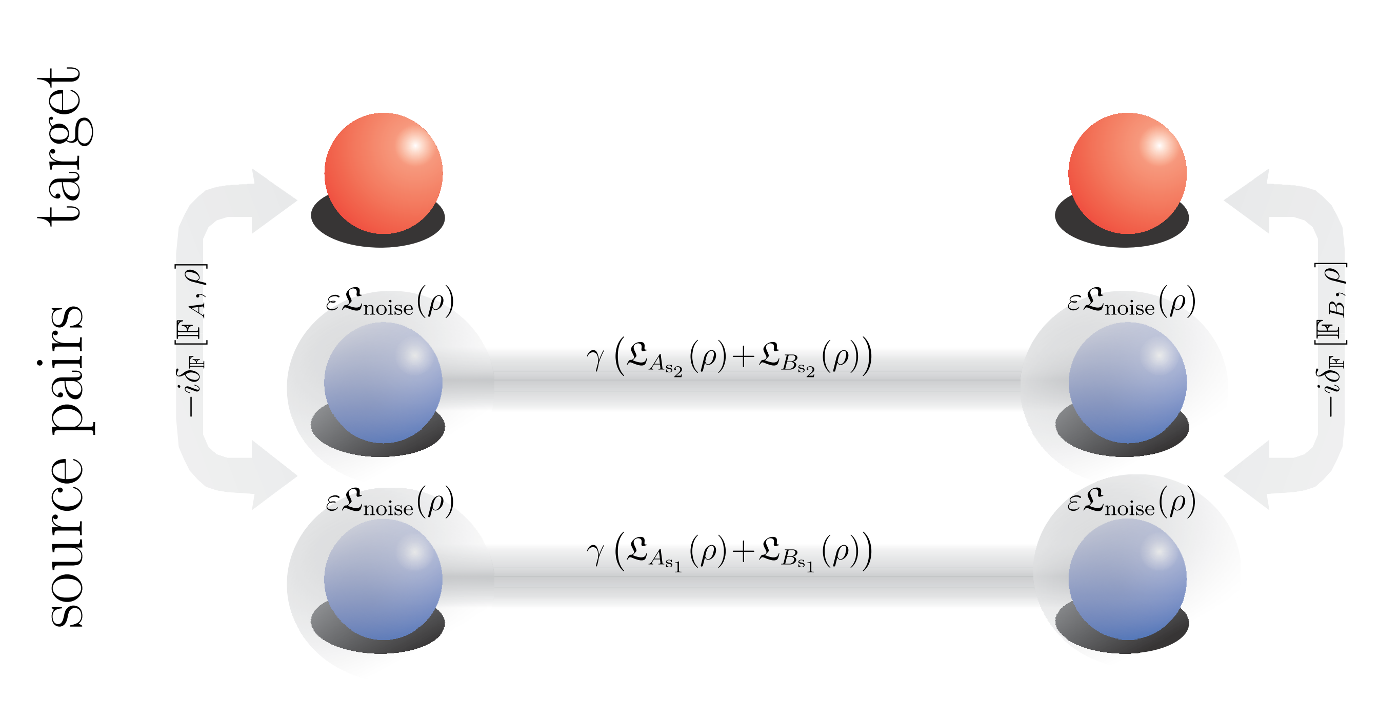
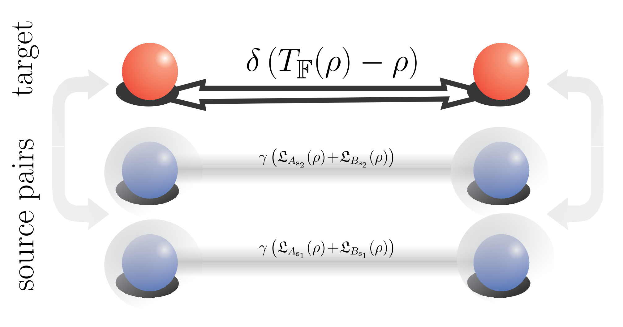
Figure 1: (Color online) Entanglement distillation by dissipation
a) Distillation setup without communication. b) Distillation setup
including classical communication.
As any other scheme, dissipative protocols are exposed to noise
sources, which degrade the quality of the produced state and
render it inapplicable for many important applications in quantum
information, like quantum communication where noise effects
increase dramatically with the distance. By means of distillation
HDistillation , entanglement can be improved at the expense
of using several copies. In combination with teleportation, this
method allows for the construction of quantum repeaters
HBriegel , which enable the distribution of high-quality
entanglement for long distance quantum communication with a
favorable scaling of resources. Unfortunately, existing schemes
for distillation and teleportation are incompatible with protocols
generating entanglement in a steady state, since they require the
decoupling of the system from the environment, such that the
advantages are lost. Hence, new procedures which are suitable to
accommodate dissipative methods such that all advantages can be
retained and used for quantum repeaters are highly desirable.
We introduce and analyze different dissipatively driven
distillation protocols, which allow for the production of highly
entangled steady states independent of the initial one and present
a novel quantum repeater scheme featuring the same properties.
More specifically, this protocol continuously produces
high-quality long-range entanglement. The required resources scale
only polynomially in the distance. Once the system is operating in
steady state, the resulting entangled link can be used for
applications. Remarkably, the time required to drive a new pair
into a highly entangled steady state is independent of the length
of the link such that this setup provides a continuous supply of
long distance entanglement HBriegel . Apart from that, the
proposed distillation protocols exhibit several intriguing
features. We present, for example, a method which allows for
distillation in steady state where none of the individual source
pairs is entangled, and describe another one whose performance can
be improved by deliberately adding noise to the system.
In the following, we introduce two types of dissipative
distillation protocols suitable for different situations. We start
out by explaining scheme I which is physically motivated and
consider the situation shown in Fig. 1. Two parties,
Alice and Bob, share two source qubit pairs s1 and s2, which
are each dissipatively driven into an entangled steady state and
used as resource for creating a single highly entangled pair in
target system . Assuming Markov dynamics, the time evolution
of the density matrix can be described by a master equation
of Lindblad form with rate and will be abbreviated by
the short hand notation
in the following. The entangling dissipative process acting on the
source qubits considered here, is the single-particle version of
the collective dynamics realized in HEbD_Experiment and
corresponds to the master equation
with and , where
and .
The unique steady state of this evolution is the pure entangled
state , where . It
is subject to local cooling, heating and dephasing noise described
by .
We assume that the entangling dynamics acting on s1 and s2
is noisy, while the target system is protected (this assumption
will be lifted below). The source qubits are locally coupled to
such that
where acts only on Alice’s (Bob’s)
side.
We choose
, corresponding
to the unitary evolution with respect to the Hamiltonian
, where and
.
Note that this distillation protocol does not require any
classical communication or pre-defined correlations. As can be
seen in Fig. 2a, the efficiency is mainly
determined by the mixedness of the source states rather than their
entanglement. In the absence of errors, the target system reaches
a maximally entangled state.
Figure 2: (Color online) Dissipative distillation according to
scheme I without communication (panel a) and including classical
communication (panels b-d). The full red lines show the steady
state entanglement of formation (Eof) of system . The dashed
blue lines depict the steady state Eof of the source state s1
if no distillation is performed (a,c,d) and during the protocol
(b). For better visibility the blue dashed curve is multiplied by
a factor 30 in panels b and c. The dotted green lines show the
entropy of s1 which is a measure of its mixedness. a) EoF
attainable without communication versus error rate
.
b) EoF versus the noise parameter . c) EoF versus
error rate . The black dotted curve represents
the entanglement of the total source system measured in log
negativity. d) EoF versus the parameter
.
In order to allow also for noise acting on , we include now
classical communication. As shown in the appendix, any Lindblad
operator of the form
where is an arbitrary LOCC channel
HLOCC , can be realized using local dissipative processes in
combination with classical communication
HRetardationFootnote .
In particular, this allows for the stabilization of the
distillation schemes discussed below against errors acting on the
target system by running them using blocks of source pairs,
which are all coupled to the same target state (see Sec. 3 in
supp ) as illustrated in Fig. 3a. If sufficiently
many source-blocks, , are used, the dynamics is dominated by
the desired processes. For clarity, we discuss the following
distillation schemes in the absence of target errors, which
corresponds exactly to the limit .
Thus, we consider the master equation
The LOOC map is defined by the four Kraus
operators , where are the
projection onto the one excitation subspace and its orthogonal
complement. Alice and Bob measure the number of excitations on
their side. After successful projection onto the subspace with one
excitation , a flip operation is
performed, in the unsuccessful case no operation is carried out.
As shown in Fig. 2b, the scheme is robust against
local noise of cooling-type
(). This kind of noise can
even be used to enhance the performance of the distillation
protocol in the steady state at the cost of a lower convergence
rate. Thus, counterintiutevly, it can be beneficial to add noise
to the system in order to increase the distilled entanglement.
Moreover, the steady state entanglement of the source pairs is
zero in the absence of cooling noise for the parameters considered
in Fig. 2b, if no distillation scheme is
performed. For increasing , the entanglement in
s1 and s2 increases, reaches an optimal point an decreases
again. Yet, the entanglement that can be distilled from these
pairs is monotonously increasing and displays a boost effect.
Panel c also hints at another counterintuitive effect, namely that
entanglement can be distilled even though none of the source pairs
is (individually) entangled in the steady state. This can be
explained by noticing that the two-copy entanglement can be
maintained for high noise rates when the single-copy entanglement
is already vanishing.
Fig. 2d shows that the distilled entanglement
increases considerably for small values of the parameter
despite the decrease in the entanglement of the source pairs. This
is due to the fact that the protocol is most efficient for source
states close to pure states, where it allows one to distill
quickly highly entangled state.
In settings where the source states can be highly mixed, another
distillation scheme (scheme II hereafter) is a method of choice
and will be explained in the following.
We analyze a generic model, which can be solved exactly and allows
one to reduce the discussion to the essential features of
dissipative entanglement distillation. As in standard distillation
schemes, we study the general problem in terms of Werner states
HWernerStates , since many situations can be described this
way and a wide range of processes can be cast in this form by
twirling HWernerStates . Werner states are of the simple
form , where
is a projector onto the maximally entangled state
, and the identity operator.
We assume a process which drives each source pair into the state
,
. Local depolarizing noise is added in the form of
the Lindblad term
where ()
denotes the reduced density matrix of Alice’s (Bob’s) system and
the normalized identity. This term describes the continuous
replacement of the initial state by the completely mixed one The
source system reaches the steady state
of the total master equation at least exponentially fast in
(see Sec. 4 in supp ).
Figure 3: (Color online) Building blocks of a dissipative quantum
repeater. a) Noise resistent distillation setup. The process
acting on the target system is boosted using several copies of the
source system. b) Continuous entanglement swapping procedure.
A continuous distillation process based on a standard protocol
HWernerDisst can be constructed considering source
pairs which are independently driven into the steady state
and a target system .
is coupled to the source pairs by a dissipative dynamics of
the form , where the completely positive map
corresponds to a process which acts on the source
pairs and distills a single potentially higher entangled copy. The
output state is written on , while the source pairs are
re-initialized in the state . The total master equation is
given by
where , denote entangling and noise processes on the
th source qubit pair.
The steady state has a fidelity of ,
where and are the fidelity of and the output of the
distillation protocol with input states of fidelity . High
fidelities require low values of . However, the
solution (see supp , Sec. 4) shows that fast
convergence requires high values of this parameter. A low
convergence speed on the target system is extremely
disadvantageous if noise is acting on . Therefore, a boost of
the process as illustrated in Fig. 3a is required. This
way, the new convergence rate is given by
while the back action on each source system remains unchanged (see
supp , Sec. 3).
The distribution of entanglement over large distances is one of
the big challenges in quantum information science. In quantum
repeater schemes, entanglement is generated over short distances
with high accuracy and neighboring links are connected by
entanglement swapping. This procedure allows one to double the
length of the links, but comes at the cost of a decrease in
entanglement for non-maximally entangled states. Therefore a
distillation scheme has to be applied before proceeding to the
next stage, which consists again of entanglement swapping and
subsequent distillation.
The basic setup for a continuous entanglement swapping procedure
is sketched in Fig. 3b. It consists of three nodes
operated by Alice, Bob and Charlie, where Alice and Bob as well
as Bob and Charlie share an entangled steady state. By performing
a teleportation procedure, an entangled link is established
between Alice and Charlie and written onto the target system,
while the source systems are re-initialized in the state .
This corresponds to LOCC operation .
The whole dynamics is described by the master equation
The steady state has a target fidelity of , where is
the output fidelity of the entanglement swapping protocol for two
input states with fidelity (see supp , Sec. 5).
The basic idea of a nested steady state quantum repeater is
illustrated in Fig.4. At the lowest level, entangled
steady states are generated over a distance . At each new
level, two neighboring states are connected via a continuous
entanglement swapping procedure and subsequently written onto a
target pair separated by twice the distance. The distillation and
boost processes, that are required in each level to keep the
fidelity constant are not shown in this picture.
The resources required for this repeater scheme can be estimated
as follows. Entanglement swapping processes acting on source pairs
of length with fidelity result in entangled target pairs
of length , with degraded fidelity . This
reduction is due to the swapping procedure, noise acting on the
target system and the back-action from entanglement distillation.
Stabilization against noise acting on the target systems is
achieved by coupling each of them to copies of the source
system and requires therefore source pairs of length . In
order to obtain a fidelity , copies of
these error stabilized links are used as input for a to
distillation process. The distilled state is mapped to another
target pair of length , which also needs to be stabilized
against errors using copies of the blocks described. Hence, in
total pairs of length are required for a repeater
stage which doubles the distance over which entanglement is
distributed. For creating a link of length , source pairs are needed, where is the number of required
iterations of the repeater protocol. Therefore, the required
resources scale polynomial with . In
Sec. 5 in supp , we discuss a specific example scaling with
.
The convergence time of the total system scales only
logarithmically with the distance . Once the steady state is
reached, the entanglement of the last target system can be used
e.g. for quantum communication or cryptography. The underlying
source systems are not effected by this process and remain in the
steady state. Therefore, the target state is restored in constant
time.
Figure 4: (Color online) Steady state quantum repeater scheme.
In conclusion, we have shown how entanglement can be distilled in
a steady state and distributed over long distances by means of a
dissipative quantum repeater scheme serving as stepping stone for
future work aiming at the optimization in view of efficiency and
experimental implementations.
APPENDIX The continuous exchange of classical
communication is added in the framework of dissipative quantum
information processing, by assuming that Alice and Bob have access
to a system, which is used for communication only and considering
the master equation
States referring to the communication system at Alice’s and Bob’s
side are labelled by subscripts c and c.
Alice’s communication system is continuously measured in the
computational basis yielding the quantum state
with probability
and reset to the state , while the
communication system on Bob’s side is set to the measurement
outcome. This way, classical information can be sent at a rate
, but no entanglement can be created (see supp ,
Sec. 2).
As proven in Sec. 2 in supp , any operation that can be
realized by means of local operations and classical communication
(LOCC) can be constructed in a continuous fashion using
communication processes and , if
the rate is fast compared to all other relevant processes
including the retardation due to back and forth communication.
We thank Eugene Polzik for helpful discussions and acknowledge
support from the Elite Network of Bavaria (ENB) project QCCC, the
DFG-Forschungsgruppe 635 and the EU projects COMPAS and QUEVADIS.
References
(1)
M. B. Plenio and S. F. Huelga, Phys. Rev. Lett. 88, 197901(2002);
B. Kraus and J. I. Cirac, Phys. Rev. Lett. 92, 013602
(2004);
F. Benatti, R. Floreanini, and U. Marzolino, Phys. Rev. A 81,012105 (2010);
R. Bloomer, M. Pysher and O. Pfister, arXiv:1007.2369 (2010);
J. Cho, S. Bose and M. S. Kim, Phys. Rev. Lett. 106, 020504 (2011) (2010);
M. J. Kastoryano, F. Reiter, and A. S. Sørensen, Phys. Rev.
Lett. 106, 090502 (2011);
A. Mari, J. Eisert, arXiv:1104.0260 (2011);
J. T. Barreiro et al., Nature 470, 486 (2011).
(2) J. F. Poyatos, J. I. Cirac, and P. Zoller, Phys. Rev. Lett. 77, 4728 (1996).
(3) S. Diehl et al. Nature Phys. 4, 878 (2008).
(4) F. Verstraete, M. M. Wolf, and J. I. Cirac, Nature Phys. 5, 633 (2009).
(5) F. Pastawski, L. Clemente, and J. I. Cirac, Phys. Rev. A 83, 012304 (2011).
(6) C. A. Muschik, E. S. Polzik, and J. I. Cirac, arXiv:1007.2209
(2010), see also: A. S. Parkins, E. Solano, and J. I. Cirac, Phys.
Rev. Lett. 96, 053602 (2006).
(7)
Joseph Kerckhoff, Hendra I. Nurdin, Dmitri S. Pavlichin, Hideo
Mabuchi, Phys. Rev. Lett. 105, 040502 (2010); J. P. Paz and W.
H. Zurek, Proc. of the Royal Soc. of London. Series A 454, 355
(Jan. 1998).
(8) H. Krauter et al. arXiv:1006.4344 (2010).
(9) C. H. Bennett et al. Phys. Rev. Lett. 76 722 (1996).
(10) H.-J. Briegel, W. Dür, J. I. Cirac, and
P. Zoller, Phys. Rev. Lett. 81, 5932 (1998).
(11) LOCC channels are completely positive trace preserving maps that can be realized by means of Local Operations and Classical
Communication.
(12) We assume, that the time scales for classical communication (see appendix) are sufficiently long
such that retardation effects can be ignored.
(13) Supplemental Material
(14)
R. F. Werner, Phys. Rev. A 40, 4277 (1989); M. Horodecki
and P. Horodecki, Rhys. Rev. A 59, 4206 (1999).
(15)
C. H. Bennett, D. P. DiVincenzo, J. A. Smolin, and W. K. Wootters,
Phys. Rev. A 54, 3824 (1996).
I Supplemental Material
Here, we explain the results presented in the main text. In Sec. 1
and Sec. 2, two dissipative distillation schemes are discussed.
Scheme I is suited for settings where a dissipative processes is
available which produces entangled steady states, that are close
to pure states. If only very mixed steady states are available as
input, scheme II is preferable (which we explain in detail in
Sec. 4). In Sec. 2, the notion of continuous exchange of classical
information between two parties is introduced in the master
equation formalism and it is shown that arbitrary LOCC channels
can be realized using local dissipation and classical
communication. In Sec. 3, we explain how the continuous protocols
used here can be made robust against noise. Finally, in Sec. 5, we
analyze the dissipative quantum repeater scheme put forward in the
main text in detail.
II 1. Scheme I: Dissipative entanglement distillation for source states close to pure states
In this section, we explain two variants of scheme I
S (1). In Sec. 1.1, we discuss a protocol, which
allows for dissipative entanglement distillation without
communication. Sec. 1.2 is concerned with a related protocol,
which includes classical communication.
Both protocols produce Bell-diagonal steady states which can
further distilled using scheme II presented in Sec. 4.
II.1 1.1 Dissipative entanglement distillation without communication
We consider the setup illustrated in Fig. S.1. The
dissipative dynamics driving the two systems and is
physically motivated and can be implemented by coupling the
systems located at Alice’s and Bob’s side to a common bath, for
example the vacuum modes of the electromagnetic field
HScott+EbD_Theory ; HEbD_Experiment . The entanglement which
can be attained per single copy is limited for a given dissipative
process. Moreover these systems are subject to noise. Still, it is
possible to use these two copies as resource for creating a single
highly entangled pair in target system .
In the absence of undesired processes, the dynamics described by
the master equation
(see main text) drives systems and into the state
Alice and Bob share a maximally entangled state
in a subspace with one excitation on each side. Scheme I is based
on the extraction of entanglement from this subspace and its
subsequent transfer to the target system by means of the flip
operation , where and
.
Systems s1 and s2 are permanently driven back to an
entangled state. In contrast to standard distillation protocols
for pure states S (10), the presence of this strong
process leads to a substantial decrease in the entanglement if the
flip operations on Alice’s and Bob’s side are not applied
simultaneously. Hence, the coordination of their actions, e.g.,
using fast classical communication, seems to be essential.
Surprisingly, the desired dynamics can be realized in the absence
of communication or predefined correlations using local unitary
evolutions.
This is possible by exploiting the symmetry of the maximally
entangled state . More specifically,
is invariant under any unitary operation of the form , while less entangled pure states are not.
denotes the complex conjugate of . Such an operation can be
implemented without communication as the time evolution of a sum
of local Hamiltonians . Here, we
use the flip operation such that the corresponding master equation
is given by
where and
.
Figure S.1: (Color online) Scheme I, dissipative entanglement
distillation without communication.
The first line corresponds to the entangling dissipative process
(described by nonlocal jump operators and ) acting on the
two source systems as explained in the main text. The second line
describes the unitary coupling of the target system to the
entangled subspace of the two source systems and the last three
lines represent undesired processes. More specifically, we include
dephasing at a rate as well as noise terms,
which create (annihilate) excitations locally at the heating
(cooling) rate ().
Note that the noise types considered here also include depolarizing noise.
The
target system itself is assumed to be protected (below, a variant
of this scheme is described, which includes classical
communication and can be made robust against noise acting on the
target system).
A disadvantage of the unitary evolution employed here lies in the
fact that the source system is subject to a back-action of the
target state, which depends on the quantum state of .
Accordingly, the evolution of the source systems is highly
dependent on the state of the target pair. It remains an open
question, whether schemes, similar to the one described in Sec. 3
can be used to render this protocol robust against errors on the
target system, or whether this is a special feature of protocols
including classical communication.
II.2 1.2 Distillation using scheme I including classical communication
Figure S.2: (Color online) Scheme I, dissipative entanglement
distillation including classical communication
channels.
We consider the setup illustrated in
Fig. S.2. As explained in Sec. 1.1,
the dissipative entangling process acting on the source systems
and has the property that Alice and Bob share a
maximally entangled state
if the resulting steady state is projected onto the subspace with
one excitation on each side. Ideally, this quantum state is then
transferred to the target system by means of the flip
operation defined above. In this subsection, we introduce a
classical communication channel, which allows Alice and Bob to
coordinate their actions such that flip operations on both sides
can be performed in a synchronized fashion if both sides have
successfully accomplished a projection onto the relevant subspace
with one excitation.
As explained in Sec. 2, Lindblad terms of the form , where
is an arbitrary LOCC channel
HLOCC , can be realized by means of local dissipative
processes and classical communication.
As explained in Sec. 3, this protocol is resistent against target
errors if it is coupled to sufficiently many blocks source pairs.
For simplicity, we explain here the basic protocol in the absence
of target errors, which corresponds to the limit of using
infinitely many source blocks (entanglement distillation for a
finite number of source blocks and finite error rates is analyzed
in Sec. 3 and Sec. 5).
Classical communication allows for the implementation of the
scheme outlined above. The LOCC distillation operation
corresponding to this process, , is given by
where is the projector onto the subspace
with one excitation, and the projector onto the
subspace with zero or two excitations. Note that only the first
term has an effect on the target system. The flip operation leads
to a back-action on the source system, which depends on the state
of . In order to simplify the discussion in Sec. 3, we
introduce here a slightly modified version of this protocol,
, which does not exhibit a state-dependent
back-action. This can be avoided by applying a twirl
HWernerStates on the target system prior to the flip
operation
is a unitary operation acting
on the target system only, where denote the four Pauli
matrices and is the identity. Due to the twirl, this
protocol features an enhanced back-action on the source, which is
independent from the target. It turns out that the performance of this
protocol is qualitatively the same as shown in Fig. 2 in the main
text. The total master equation is then given by
where and
.
III 2. Classical dissipative channels and dissipative LOCC
Classical channels are easier to realize experimentally than their
quantum counterparts and can for example be implemented using
optical fibers. Since classical channels are insufficient for the
generation of quantum correlations, long-range links can be
established over large distances using the toolkit of classical
error-correction. The class of LOCC operations, i.e. quantum
operations that can be performed using local operations and
classical communication, is of essential importance in quantum
information theory, especially in the context of entanglement
distillation protocols.
In this section, we introduce the notion of classical channels in
the framework of dissipative quantum information processing. This
allows us to formulate generalized LOCC operations in a continuous
dissipative setting, which includes a wide range of continuous
distillation protocols.
III.1 2.1 Classical dissipative channels
We start out by introducing a dissipative classical communication
channel.
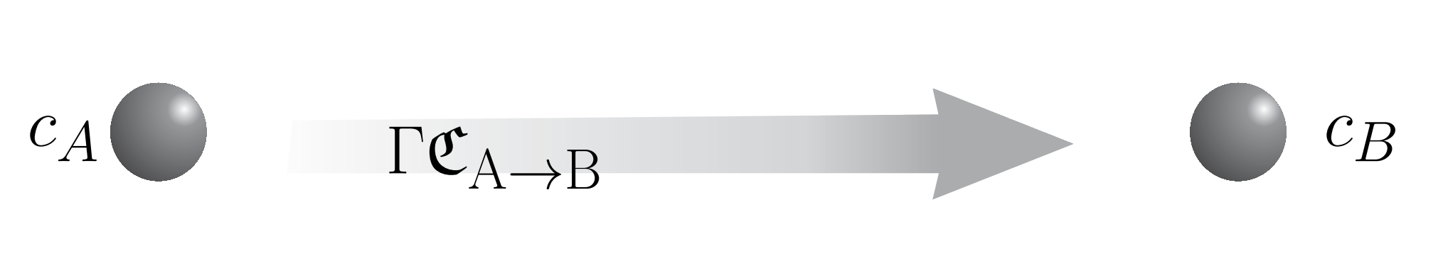
Figure S.3: (Color online) Realization of a classical dissipative
channel.
Both parties, Alice and Bob, each have access to a -dimensional
system which is used exclusively for classical communication (see.
Fig. S.3). The master equation
describes a one-way classical communication channel. States
referring to the communication system at Alice’s and Bob’s side
are labelled by subscripts c and c
respectively. Alice’s communication system is continuously
measured in the computational basis yielding the quantum state
with probability
and reset to the state , while the
communication system on Bob’s side is set to the measurement
outcome. This process can be written in the form
where the completely positive map is an entanglement
breaking operation S (2), which maps any state to a
separable one. The solution of this master equation is
given by
The second term is separable, since is entanglement
breaking. Accordingly, the classical channel introduced above does
not produce entanglement. Moreover any entanglement present in the
state is exponentially suppressed.
III.2 2.2 Generation of Lindblad operators of the form
In the following we prove that any dissipative time evolution
which satisfies a master equation of the form can be designed by means of local
dissipative processes in combination with the classical
communication channels introduced above in the limit of high rates
. The basic setup is sketched in Fig. S.4.
Alice and Bob hold a bipartite system, which we refer to as the
main system. In addition both parties have access to several
classical communication channels and can apply dissipative
dynamics acting on the classical channels and their part of the
main system. This setting allows for a wider class of dissipative
evolutions on the main system which includes dissipative LOCC
processes. In particular we state the following:
Let be any LOCC map. Let be any
bounded Lindblad operator, i.e., , acting on the main system at a rate . Let Alice and
Bob have access to classical communication channels as described
above. If both parties can apply any dissipative process of
Lindblad form on their side, an effective dissipative time
evolution on the main system satisfying the master equation
(1)
after an initial waiting time of the order can
be realized. The completely positive operator
is an
imperfect realization of up to an error
, which vanishes for small
, where
. denotes
any hermitian (time and state dependent) operator with a trace
norm scaling with in the limit .
Since , the strength of
the process is completely encoded in .
can include a dissipative LOOC map itself, as
discussed at the end of this section. The error
of the LOCC map is small for
.
A time evolution satisfying Eq. (1) can be either
obtained by starting from certain initial conditions, or after an
initial waiting time on the order of , during
which no external control is required.
If (), the
system evolves approximately according to .
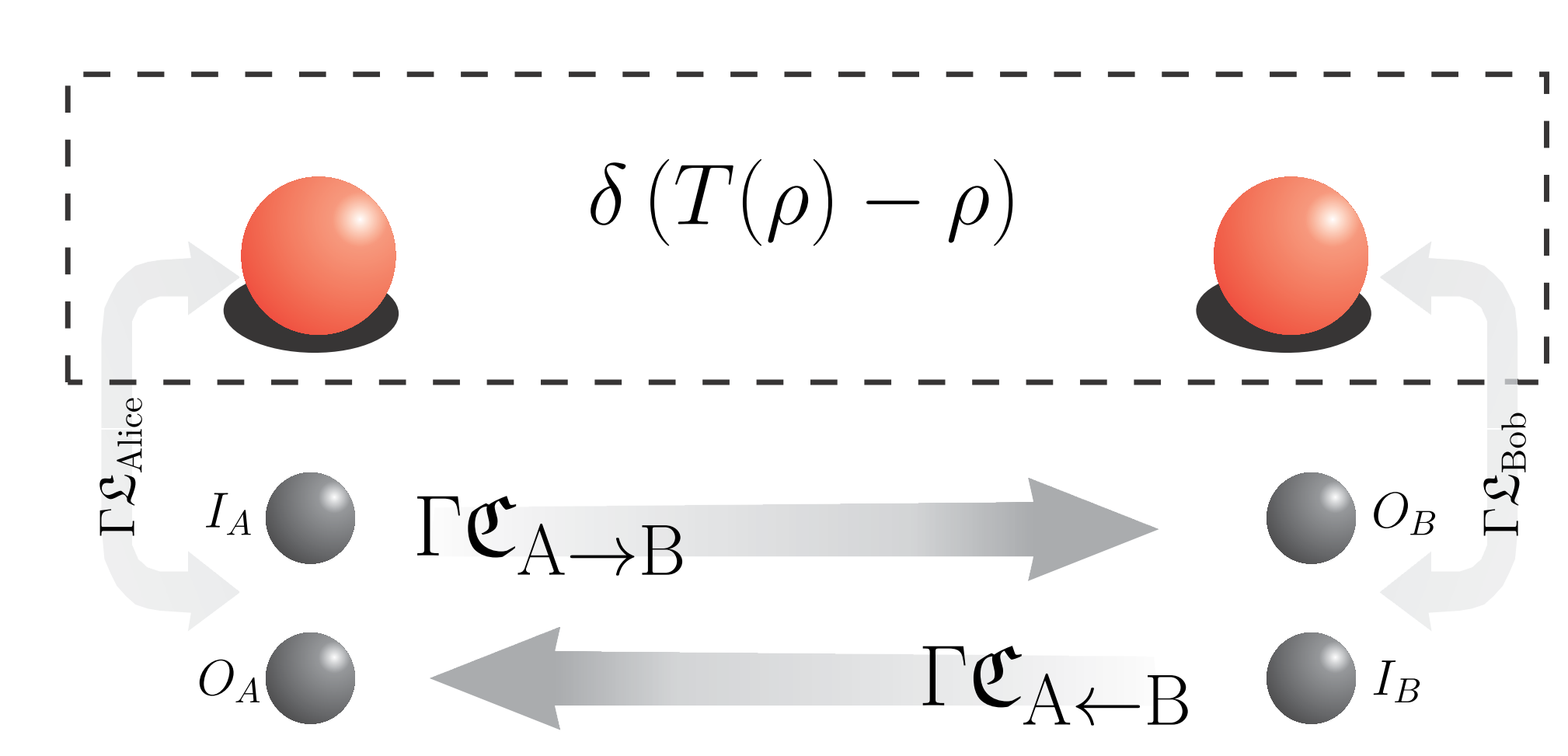
Figure S.4: (Color online) Using local dissipative processes and fast
classical communication, arbitrary LOCC channels can be
implemented in a continuous fashion.
Note, that LOOC operations are extremely hard to parameterize. It
is known, that they can be written as a separable superoperator
, but
not every separable superoperator is a LOCC map. Practically, a
general LOCC map can only be characterized by fixing the number of
communication rounds between Alice and Bob and to specifying the
exact operations that Alice and Bob perform in each round. The
most general operation Alice and Bob can apply is a positive
operator valued measurement (POVM). This covers any completely
positive map as well as measurements, unitary evolutions, etc. A
POVM is specified by a number of Kraus operators ,
corresponding to the possible measurement outcomes , where the
normalization condition guaranties
that the probabilities for the different possible outcomes add up
to .
We consider the following situation. Alice performs a first POVM
and sends her result to Bob. Bob chooses a POVM
depending on Alice’s result . Subsequently, he sends
the result to Alice, who chooses her next POVM
which may depend on all previous measurement result. This
procedure can be repeated many times. This corresponds to the
application of the operation
where each Kraus operator is of the form
and represent one possible set of measurements outcomes for all POVM measurements. Due to
this lack of a concise notation for a general LOCC map, a complete
proof of this statement would be lost in notation and it would be
hard for the reader to understand the main idea of the proof. We
restrict ourselves therefore to LOCC maps with one communication
round, i.e., Alice sends one message to Bob and Bob can send an
answer back to Alice once.
A generalization of the following proof to a LOCC map with a
finite number of communication rounds is straight forward and
will be discussed below.
Let denote a LOCC map with one round of
communication. This map can be realized in the following way:
•
Alice applies a POVM measurement with Kraus operators , obtains the measurement result and sends it to Bob.
•
Bob performs a POVM measurement , which can depend on , and sends the result
to Alice. Since we assume that Alice is memoryless, Bob also sends the measurement outcome of Alice’s measurement .
•
In the last step, Alice can apply any completely positive map on her side. This map can depend on both, and .
Note, that is also a POVM map with Kraus operators
, where the measurement results are not used. Let
Alice and Bob have different measurement results for each
POVM, where can be upper bounded by the square of the
dimension of the system. For typical distillation protocols on
qubits, . Note that all indices for Kraus operators run from
to , and do not start with . This choice allows for a
shorter notation later on (the index is reserved for
indicating that the classical channel is operable). The basic
setup is illustrated in Fig. S.4. Alice and Bob have
access to classical one-way communication channels labelled
and . and can be used to send information from Alice
to Bob and vice versa respectively. Apart from these classical
channels, Alice and Bob hold a system subject to a dissipative
evolution described by the Lindblad operator .
In the following, this system is referred to as the main system.
The first classical channel needs to store all possible
measurement outcomes obtained by Alice, whereas the second one
needs to store the measurement results obtained by both, Alice and
Bob. We assume therefore that and are and
dimensional systems respectively. Note, that the
state will be used to indicate that the channel input or
output is ”empty”, while the states
represent possible measurement results of Alice and the states
encode the different measurement
results obtained by Alice and Bob. The corresponding master
equation is given by
where is a process acting on the main
system only. We assume, that the time scales for classical
communication are sufficiently long such that
retardation effects can be ignored. The four systems used for
classical communication are denoted by as shown
in Fig. S.4. and stand for ”Input” and
”Output”.
As a next step, local Lindblad operators are added, which
correspond to the application of a LOCC map depending on the
registers of the classical channels. The following three terms are
added, one for each step of the protocol outlined above. The first
term is given by,
where acts on Alice’s part of the main system and
on Alice’s side of the first classical
system, i.e., the input system of the first classical channel.
Note, that we use here the short hand notation
that was
already introduced in the main text. This corresponds to the first
step of the realization of the LOCC map. Alice performs a POVM and
writes the measurement result onto the input system of the
classical channel. As second term, we add the Lindblad operator
where acts on Bob’s part of the main system,
on the output of the first classical
channel and on the input of the second
channel. Note, that the second channel can store both values
and at the same time. stands for any encoding of
in the dimensional state space, where the label zero
is reserved for indicating the status of the channel. The
summation over starts from zero, i.e., includes the reserved
zeros term as well as the possible measurement results. Bob
only carries out a POVM measurement, if he receives the message
via . Afterwards he writes onto the classical
channel. Note that the sum over implies that Bob overwrites
any previous state of the classical communication system. The last
term to be added is given by
where acts on Alice’s quantum system with
and
act on the output of the second classical
channel. Alice receives the message and reacts by applying
to complete the LOCC map. The sum starts from ,
i.e., Alice acts only if a message has arrived. She does not act
if the register is empty (). Hence, the total master
equation is given by
The basic idea can be described as follows. The term in the second
line starts the process of realizing at a rate
(Alice performs the first step). The following steps are performed
with a high rate , such that the state of the quantum
system stays approximately constant during the time needed to
complete the whole operation. So, practically, the whole LOCC map
is applied at once at a rate .
In the following, this will be proven rigorously by considering
the effective evolution of the main systems after tracing out the
classical channels. The reduced state of the main system can be
written as
with , where , (, )
denote the computational bases for (). The indices are
arranged such that their order corresponds to the order in the
communication cycle. refers to the input of Alice’s side,
to the output on Bob’s side, to the input on Bob’s side and
to the output on Alice’s side. A system of differential
equations for all can be derived using
and
Eq. (III.2).
The desired terms
evolve according to
(3)
(4)
(5)
(7)
All other terms correspond to small errors. In the first step of
the proof it is shown that after an initial waiting time, only the
states
are significantly populated, while the population of all other
states is small.
In the next step it is shown that . In
the following we will use the short-hand notation
.
III.2.1 Bounds for occupation probabilities
Let us define the probabilities . A
system of differential equations
for these probabilities
can be derived by from the differential equations for
. Traceless terms such as and do no longer appear.
We define as the sum of
, where all indices marked with are summed from
to , in order to remove the dependence on the Kraus
operators by virtue of their normalization condition (). A successful application of the
LOCC map corresponds to the series (similarly to a X-excitation which created on
the first index, travels to the right and disappears in the end).
takes high values, while the other probabilities are on
the order of , which indicates that this
process is fast. However, the situation considered here does not
correspond to this ideal case because Alice can start a new round
before the last one is finished, which gives rise to probabilities
which are denoted by indices with more than one , e.g.
which results in an incorrect
realization of the LOCC map.
Since we are not interested in the complete solution but only in
upper and lower bounds, we further simplify the system by defining
the probabilities
and ,
which cover all possible events. indicates that the
corresponding index is different from zero. Therefore, the
summation runs from to . stands for an arbitrary
value, i.e., the summation starts from zero. These five quantities
include also non-ideal process, with two or more X entries which
correspond an errors and evolve according to
The solution shows that the steady state (ss) with
(8)
is reached up to an error smaller than
after a time of the order of
S (3). In the steady state,
.
Next, bounds for are
derived. According to Eq. (4),
.
Assuming that is reached after a time
,
where is a positive function since
. Hence, doubling the initial waiting time
guarantees .
According to Eq. (5), . By integration, using the bound
for and assuming that the contributions from
and sum up to a positive function we
conclude that is fulfilled
after waiting for another period on the order of
. Similarly, one obtains and .
Since
, any probability with more than two
entries is smaller than . In
summary,
after a time of the order , where the upper
bounds are found using Eq. (III.2.1). Hence, a steady state is
reached where states labelled with one (more than one) are
occupied with probability ().
III.2.2 Differential equation for
The evolution of is governed by
Eq. (LABEL:Eq:MEtotal). After a period of the order
, since
.
Hence, for , is approximately constant on
time scales that are short compared to .
In order to obtain an equation which depends only on , we
solve successively the differential equations for
and
. According to Eq. (4),
where , which is bounded by . For the first three terms we use
, the last term can be bounded by
such that
The integral can
be bounded by . The initial term is
suppressed by and therefore smaller than
after the initial waiting time. Hence,
(9)
Since the integral is mainly determined by terms close to and varies little on small time intervals,
can be assumed to be constant. To prove this, we consider
(10)
with and . Since
is the typical time during which
changes, it is nearly constant during the interval . From
, we obtain that
for any
(11)
The integral from to in Eq. (10) are suppressed
at least by a factor ( is on the order of one). Inserting
Eq. (11) in Eq. (9) and using
with yields
(12)
which shows that for small , Alice applies her first POVM
with high accuracy.
where can be bounded by
using
,
and
. Inserting
Eq. (12) yields
.
As before, the integral over and the first term can
be bounded by after a waiting time. If the
remaining integral is split as in Eq. (10), we obtain one
part, where is nearly constant and one vanishing part.
The main error is again due to expression (11),
leading to
(14)
Hence, for small , sending classical information to Bob
causes only marginal errors on the main system.
which corresponds to a process, where Bob applies his part of the
POVM and writes onto his classical input register.
Similarly, Eq. (7) leads to
which corresponds to a transfer of the classical measurement
results back onto Alice’s side. Finally, these results can
be applied for calculating ,
represents a
noisy version of the desired LOCC map . The undesired
contribution can be suppressed by choosing small, i.e. by
choosing large enough.
The generalization to more than one round of communication is
straight forward. By summing over the indices of the corresponding
Kraus operators, one obtains equations for the probabilities,
which are independent of the POVMs applied in the protocol. From
these equations it can be concluded that only the relevant state
responsible for the application of the LOCC is populated, while
all others are suppressed by a factor of order after a
initial waiting time. By successive integration as shown above,
the desired approximation for is obtained. Many
distillation protocols only require only a small number of rounds
to reach high fidelities and often even only one-way communication
(half a round) [9,15].
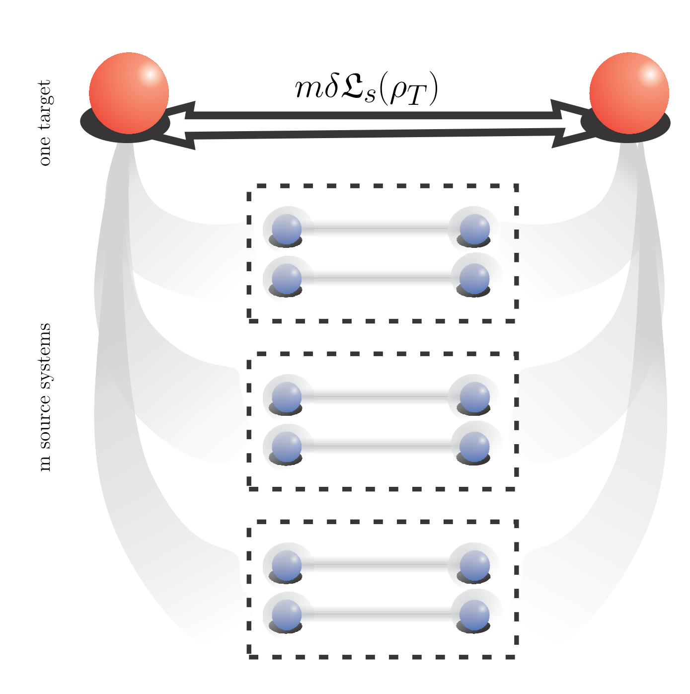
IV 3. Stabilization of dissipative distillation schemes against errors acting on the target
system
Figure S.5: (Color online) Stabilization of dissipative protocols
against noise acting on the target system by coupling several
source system to the same target.
In this section, we explain how the distillation schemes presented
in Sec. 1.2 and Sec. 4 can be made robust against noise acting on
the target system. The same method for stabilization against
errors is applicable for both protocols and a wide range of other
dissipative schemes, which include classical communication.
The basic idea is illustrated in Fig. S.5. A
dissipative protocol is run using blocks of source systems in
parallel, which are all coupled individually to the same target
system. This way, a boost effect on the desired dynamics of the
target system can be achieved, while the back-action on the source
pairs remains unchanged. If sufficiently many source systems are
provided, the dynamics on the target system is dominated
completely by the desired dynamics.
In the following, we explain the application of this method first
for schemes of the type described in Sec. 4 and 5 and discuss then
briefly the stabilization of scheme I.
We start out by considering a target system and a source
block consisting of pairs. An entangling dissipative process
described by the Lindblad operator
acts on each source pair separately such that each of them is
individually driven into an entangled steady state . The
effective master equation for the target system, which is obtained
by tracing out the source system, is given by
where the Lindblad operator may be time
dependent. It does not depend on the state of but only on the
state of the source system as indicated by the subscript .
Accordingly, the convergence speed at which
converges to a constant operator is
given by the rate at which the source system reaches a steady
state. The convergence rate of the source system is limited by the
rate at which the flip operation mapping the quantum
states of the source system to is performed (see
Sec. 1 and Sec. 4).
We assume that identical source system are
individually coupled to a single source system through the
Lindblad operator ,
where is a Lindblad operator acting
on and the th source system (see Fig. S.5
for a schematic overview). We assume that these operators are
identical such that the
dynamics of the target system is governed by the reduced master
equation
This is not generally the case, since the source systems are
coupled to each other through the target system. Due to this
indirect coupling, the source systems may evolve differently in
time and can reach different steady states, which can be
disadvantageous for the evolution of the target system. This is
for example the case for the scheme described in Sec. 1.1 which
does not include classical communication.
It can be shown that
, if there
is no state dependent back-action of on the source systems.
In this case, the evolution of the reduced density matrix of each
source block is independent from the time evolution of the other
blocks. This property can be guaranteed by re-initializing the
source systems after each swap operation in a standard state, for
example the identity (strict equality requires in principle also
that all source systems start from the same initial state.
However, different initial states have only an effect on the time
evolution in the beginning. The following discussions are only
concerned with the steady state of the system, which is
independent of the initial conditions).
Scheme I including classical communication (see Sec. 1.2) exhibits
a weak state dependent back-action. As explained in the end of
Sec. 1.2, this can be avoided by applying a twirl
HWernerStates on the target system prior to each flip
operation. Hence, the stabilization method outlined above is
directly applicable to this modified version of the scheme
S (4).
By boosting the desired dynamics on the target system, arbitrary
high error rates can be tolerated. For , the dynamics governed by the master equation
is dominated by the first term and the steady state is arbitrarily
close to the original steady state.
In the specific case, where the process driving the target system into
the steady state is counteracted by depolarizing
noise , the time evolution described
by
leads to the steady state , which can be easily
verified by solving the equation . This state is
reached exponentially fast with a rate .
The same result holds for local depolarizing noise acting on
Alice’s and Bob’s system (see Sec. 4.1) if the steady state
is a Werner state. A master equation of this type
is solved exactly in the next section.
V 4. Scheme II: dissipative entanglement distillation for Werner states
In this section, we introduce a second dissipative distillation
scheme, which does not rely on entangling processes producing
steady states, which are close to pure states, as scheme I
presented in Sec. 1.
We analyze here a very general model for Werner states
HWernerStates , which can be solved exactly. Werner states
are of the simple form , and are characterized in terms of their
fidelity , which is given by the overlap with the maximally
entangled state .
Any quantum state can be transformed into a Werner state by
twirling HWernerStates without a loss of fidelity. Since a
Werner-twirl is a LOCC map, a dissipative protocol can be
constructed, which corresponds to the continuous application of a
twirl operation on a given system and mapping of the resulting
state to a new pair acting as target system by means of a
continuous flip procedure (compare Sec. 4.2).
This way, any dissipative process can be modified such that it can
be described in terms of a Werner Lindblad operator
as used in Secs. 4 and 5, where is the steady state fidelity
of the underlying process. In this sense, the Werner model used
here is very general and can be applied in many situations.
V.1 4.1 Dissipative entangling model process for a single source pair
A dissipative model process, which produces an arbitrary Werner
state as steady state can be modelled by considering two
processes, which generate the steady states and
respectively, where denotes the normalized identity. Let
denote the four Bell-states, where
, and
the Pauli matrices, where is the identity. A
master equation which leads to the steady state
can be constructed using the
four jump operators ,
which give rise to the Lindlbad term
Similarly, a master equation which leads to the steady state
is obtained using the jump operators , which give rise to the Lindblad term
Hence, the Werner state with fidelity is the
steady state of the time evolution governed by the master equation
The Lindblad term will be used in the following to
model the basic entangling process acting on the source systems.
Local depolarizing noise acting on Alice’s (Bob’s) side is
included using the jump operators
(),
such that the corresponding Lindblad
terms are given by
where () is the reduced density
matrix corresponding to Alice’s (Bob’s) system and ()
the normalized identity on Alice’s (Bob’s) system. This
process describes the continuous replacement of the state on
Alice’s (Bob’s) side by the completely mixed state. The total
master equation
(15)
where
,
describes the basic entangling process including local noise. This
type of equation will be used frequently in the following
sections, as it also describes also the evolution of the target
systems once the corresponding source systems have reached the
steady state.
The steady state of the time evolution described by
Eq. (15) is a Werner state
(16)
with reduced fidelity .
The general time dependent solution of the master equation
(15) is of the form
(17)
where is any initial state,
, and . and are the reduced density matrices of the initial
state at Alices and Bobs side.
The functions are given by
(18)
where and . Note,
that the terms which depend on the initial state of the system,
i.e. and , are suppressed exponentially fast. The
system reaches the steady state given by
Eq. (16) exponentially fast with a rate
of at least .
In order to verify that Eqs. (17) and (V.1) are a
solution of Eq. (15), Eq. (17)
can be used as ansatz. The master equation gives rise to a set of
differential equations for the functions with initial
conditions and ,
(19)
Below, the initial condition will be considered
frequently. In this case the solution simplifies to
(20)
V.2 4.2 Steady state entanglement distillation acting on source systems
We consider systems which are subject to the basic entangling
process and are driven
into the steady state as described in Sec. 4.1.
These qubit pairs act as source systems for a LOCC distillation
operation , which distills one potentially higher entangled
state from these copies. The resulting quantum state is mapped to
a target pair and each source system is
re-initialized in the state . We do not specify at this
point - the solution derived in this section holds for any to
distillation protocol. We start out by considering only
deterministic protocols and generalize the results at the end of
this section such that probabilistic schemes are also covered.
Note that the complete re-initialization of the source systems
represents the worst-case situation regarding the back-action
of the target system onto the source pairs. This choice allows us
solve the model exactly and to provide a lower bound for
dissipative distillation schemes of this type.
The continuous distillation procedure explained above is
described by the master equation
(21)
where stands for the dissipative process
acting on the th source system.
In the following, we determine the time evolution and the steady
state of the target system. The reduced master equation for depends on the steady state of the reduced source
system. Therefore, we start by solving the dynamics on the source
system. Since the back-action of on the source
system does not depend on the quantum state of , the
time evolution of the source pairs can be considered independently
from the target system.
For clarity, the reduced states of source and target system are
denoted by and respectively in this section.
The reduced master equation for the source systems is given by
(22)
The solution of the homogeneous master equation which describes
the entangling dynamics for independent source systems
is already known (see Sec. 4.1) if the initial state is a product
state. denotes the solution of the
homogeneous master equation with initial condition
.
The solution of the inhomogeneous master equation
Eq. (22) is given by
with arbitrary initial condition . This
solution can be easily verified by considering the time derivative
is reached exponentially fast with a rate of at least .
The homogeneous solution is given by
the tensor product of the solution for a single source pair
(20),
Next, we consider the dynamics of the target system
described by the time dependent master equation
which is solved by
with steady state . The corresponding steady state
fidelity can be inferred by integrating over the fidelities that
are obtained if a standard distillation protocol is applied such
that
So far, it has been assumed, that the underlying distillation protocol
is deterministic, such that a distilled state is available
whenever it is applied. However, many distillation protocols of
interest are probabilistic, i.e., they only succeed some
probability .
If a probabilistic distillation protocol is used, the
corresponding map is defined in such a way, that a flip
operation is only performed when the distillation was successful,
which leads to a state dependent rate in the master equation
Accordingly, the target system is driven into the same steady
state as discussed above with a reduced rate. Once the time
evolution of the source system has reached a steady state, the
dynamics of the target system is determined by the master equation
where is the distilled steady state of the source
system. Since is a Werner state, the target system can
act as one of new source systems which drive a new target
system into an even more entangled state. This way, the
distillation protocol can be iterated in a nested form.
VI 5. Continuous quantum repeaters
The ability to distribute entangled states of high quality over
long distances is of vital importance for quantum communication
and quantum network related applications in general. As opposed to
classical information, quantum information cannot be cloned.
Therefore, classical repeater schemes are not applicable in this
context and quantum repeater schemes which respect the coherence
of quantum states are required
Briegel; DLCZ; QuantumInternet. In quantum repeater
protocols, entanglement is first distributed over short distances
with high accuracy. Then neighboring pairs are connected by
a teleportation procedure S (5) (entanglement
swapping EntaglementSwappingTh; EntanglementSwappingExp)
such that entangled links which span a distance are
obtained. In the next step, two neighboring links of length are connected by entanglement swapping, resulting in
entangled pairs which span a distance . This way, an
entangled link of length can be established in
iteration steps (compare Fig. 4 in the main text). However, for
non-maximally entangled states, entanglement swapping leads to a
considerable degradation in the fidelity of the resulting quantum
state. Since the distributed entanglement decreases dramatically
every time the length of the entangling links is doubled, it can
not be distributed over large distances this way. Therefore an
entanglement distillation protocol has to be applied after every
entanglement swapping procedure before proceeding to the next
stage.
In the following, we describe a continuous dissipative quantum
repeater scheme, which combines continuous swap and distillation
processes in order to generate long-range entangled steady states,
while entangling dissipative processes are only required over
short distances. To this end, we introduce a continuous swap
operation in Sec. 5.1 and explain in Sec. 5.2 how this method can
be combined with the distillation scheme presented above (Sec. 4)
such that a high-quality entangled link can be established over a
large distance as steady state of a continuous dissipative
evolution. We conclude this proof-of-principle study by giving a
specific example.
The basic setup for entanglement swapping consists of three nodes
aligned on a line, operated by Alice, Bob and Charlie, where
Alice and Bob as well as Bob and Charlie share an entangled pair,
while the distance between Alice and Charlie is too large for
generating an entangled state of high quality (see Fig. 3b in the
main text). By performing a teleportation procedure, which
requires the measurement of the two qubits at Bob’s node and
classical communication to Alice and Charlie, as well as local
operations on their sides, an entangled link can be established
between Alice and Charlie EntaglementSwappingTh.
We consider a setting, where Alice and Bob as well as Bob and
Charlie each hold a source pair which is subject to the basic
dissipative entangling mechanism considered in Sec. 4, such both
pairs are individually driven into the steady state . This
dynamics is described by the Lindblad term
. As illustrated in Fig. 3b in the main text, the
source pairs are coupled to a pair of target qubits shared between
Alice and Charlie through the term
, where
the completely positive map corresponds to a flip
operation which maps the state resulting from the entanglement
swapping procedure to a target system and re-initializes the
source systems in the state S (7).
Hence, the total master equation is given by
and the reduction to the source systems yields
The solution of this differential equation (compare Sec. 4.2)
where is the homogeneous solution with
initial condition , shows that the steady
state
(25)
where , is reached exponentially fast with
a rate of at least .
Figure S.7: (Color online) Dissipative quantum repeater architecture.
a) Concatenation of elementary steps, in which the distance over
which entanglement is distributed is doubled. b) Illustration of a
single iteration step including entanglement swapping and
-distillation.
The time dependent master equation governing the dynamics of the
target system is given by
(26)
where is the steady state of this
evolution. According to Eq. (25), the steady
state fidelity is given by
where is the fidelity of the state and
is the output fidelity of the swap
protocol for two input states with fidelity . A short
calculation shows that
(27)
where is the fidelity of the state and
.
As discussed in Sec. 3, the scheme can be made robust against
noise processes acting on the target system by using copies of
the source systems and coupling them all to the same target state.
VI.2 5.2 Creation of long-range, high-quality steady state entanglement
The continuous swap operation introduced above (Sec. 5.1), the
dissipative distillation protocol explained in Sec. 4 and the
method for stabilization against errors acting on target systems
(Sec. 3) are the basic building blocks for the dissipative quantum
repeater scheme illustrated in Fig. S.7.
To begin with, the distance over which an entangled link has
to be established is divided into segments of length ,
as in standard repeater schemes. At each intermediate node, many
qubits are supplied which are subject to local depolarizing noise
acting at a rate . We assume that each source pair
constituting an elementary link of length is individually
driven into a steady state of high fidelity by means of
an entangling dissipative process of the type discussed in
Sec. 4.1., , with high initial steady state
fidelity and a rate , which is large compared to the
noise rate . Note that this assumption can also be
satisfied starting from dissipative processes leading to a steady
state with low fidelity and low if distillation and boost
processes are applied as discussed above. In the following, we
consider an iteration step of the repeater protocol which acts on
entangled source systems, which each span a distance
with fidelity , and produces entangled links of the length
with fidelity , such that . This is
illustrated in Fig. S.7, where the entangled
source pairs of length are shown in blue and the yellow target
pairs of length are depicted in yellow. Each iteration step
consist out of the following subroutines, which are illustrated in
Fig. S.7b:
•
Neighboring source pairs of length (blue) are connected via a
continuous swap operation. The resulting quantum states are
written onto target pairs
(red). In order to achieve a boost-effect on the targets, this protocol is run on source systems in
parallel.
•
A block of such pairs , , acts as source system (green) for an distillation process, which maps the resulting quantum state to new target system (yellow).
•
of these blocks (green) are needed to achieve a high fidelity of the quantum state of the target systems (yellow).
This iteration step results in entangled links (yellow) which span
twice the initial distance and feature a high fidelity as well as
a high convergence rate once all source systems have reached the
steady state.
In the following, we consider
for simplicity (these
parameters can be optimized for a given distillation protocol).
The individual levels of the repeater scheme converge seriatim
from bottom to top to a steady state. For example, once the source
systems of length (blue) are in a steady state, the reduced
master equation for the target system of length (yellow)
becomes time independent and this system reaches a steady state
too.
We assume now, that all source pairs of length (blue) are
driven by a time independent master equation of the type discussed
in Sec. 4.2, once all underlying
systems have reached the steady state.
The reduced master equation for the target system
(red)
includes local polarizing noise as introduced in Sec. 4.1 and the
back-action of the distillation scheme. Note, that the rate of the
entangling process, is again high, due to the
boost on the target system. The entangling process acting on the
target systems of the distillation procedure (yellow),
is
determined by the steady state fidelity
.
A wide range distillation protocols for Werner states
S (8) can be used in a continuous form as demonstrated
in Sec. 4 (below a specific example is discussed). As explained
there, a distillation protocol corresponds to a completely
positive map which is described by a Linblad term
. The distillation
process is applied continuously for each entangled link and the
resulting highly entangled qubit state is flipped to new target
pairs spanning the same length .
We consider here a distillation procedure which acts on
entangled source systems and distills one potentially higher
entangled pair. Hence, for each of the links, copies
, ,
have to be supplied. This situation is sketched in
Fig. S.7b, where the target systems
(red), driven by the source pairs
(blue), are used as resource for creating a highly entangled
steady state of the new target pair (yellow). One source block
(shown in green) is sufficient for entanglement distillation, but
several of them running in parallel are needed to boost the
desired dynamics on the target system.
This way, each target pair is driven at
a rate and the total effective master
equation for the target systems of the distillation protocol is
given by
Hence, the resulting steady state fidelity is
where is the entanglement
distilled from source systems with steady state fidelity
.
In order to iterate this process, we require
, which can always be achieved
using a strong entanglement distillation (large ) and high
entangling rates S (9).
The next iteration step begins with another continuous
entangling swapping procedure. Here, the target systems of the
distillation scheme act as source systems for the entanglement
swapping operation.
Since the total distance has been divided into segments (
), the protocol has to be iterated times. As
explained above, each iteration stage requires qubit pairs
such that in total source systems are
needed. Hence the resources scale with
in the distance. We restrict the estimate of the required
resources to the number of used qubit pairs, since the other
resources scale polynomial in this quantity.
As specific example we consider the distribution of an entangled
state such that each repeater stage starts with and results in
links with fidelity . We consider noise acing at a rate
, distillation based on source systems (the
distillation protocol is described below) and stabilization of the
target pairs by means of copies of the underlying source
blocks and . In this example, the required
resources scale with
.
The entanglement distillation scheme used here is a four-to-one
distillation protocol for Werner states S (8) which is
applied two times in a nested fashion. Starting from four source
states , , , with fidelity ,
the following operations are performed. First, a bilateral
operation is applied to the
first two pairs (where is the control and the target
qubit ) and is measured in the computational basis. Then, a
Hadamard transformation is performed on both qubits of .
Subsequently, a bilateral
operation is applied to the first and third pair (where is
the control and the target qubit) and is measured in
the computational basis. The measurement obtained on Alice’s and
Bob’s side are compared. If their measurement results coincide,
the resulting state is the desired higher entangled state.
If not, the ”safety-copy” is used instead. In this event,
distillation was not successful and the fidelity has not been
increased, but in any case an entangled pair is available.
The fidelity of the resulting state is given by
where and
is the success
probability of this protocol. In the example above, this protocol
is applied twice in a concatenated fashion. The second application
of the scheme is run using the output states of the first one as
input such that
.
We conclude this section with an estimate of the convergence
speed of the presented repeater scheme. We start by considering
the elementary pairs constituting the entangled links on the
lowest level of the scheme. These systems reach the steady state
up to a certain high accuracy after a time . After this time,
the dynamics of all systems on the next level is governed to a
good approximation by a time independent master equation and
converge with high accuracy to the steady state after another time
period of length has elapsed. Convergence of all levels
of the repeater scheme requires therefore a waiting time .
Since the number of levels used in the scheme scale only
logarithmical with the distance, we obtain a very moderate scaling
of the convergence time with the distance.
Note, that once the whole system is in a steady state, removal of
the final long-range entangled pair does not have an effect on the
underlying systems which remain in steady state.
The repeater protocol put forward here is based on continuous LOCC
maps, which represent a particular subset of possible dissipative
schemes. We have also presented a distillation protocol (scheme
I), without communication which does not fall in this class.
However, also the set of dissipative processes assisted by
classical communication includes other types of schemes not
covered here, which are yet to be explored.
References
S (1)
The variant of scheme I without communication is fundamentally
different from scheme II, presented in Sec. 4 and cannot not be
formulated in terms master equations of the form
, where is a
LOCC channel.
S (2)
M. Horodecki, P. W. Shor, and M. B. Ruskai, Rev. Math. Phys.
15, 629 (2003).
S (3)
The slowest term converges as . After
an initial waiting time of the order of the
steady state is reached up to an error of the order
.
S (4)
It can be shown that this back-action has only a small effect on
the steady state of the source system, and not accumulate if many
source systems are coupled to . If the parameter is
small, the back-action can be bounded several source system can be
combined as described above. The strict avoidance of a state
depended back-action is enforced only for the sake of clarity.
S (5)
C. H. Bennett et al, Phys. Rev. Lett. 70, 1895 (1993).
S (6)
M. Żukowski, A. Zeillinger, M. A. Horne, and A. K. Ekert,
Phys. Rev. Lett. 71, 4287 (1993); J.-W. Pan, D.
Bouwmeester, H. Weinfurter, and A. Zeillinger, Phys. Rev. Lett.
80, 3891 (1998).
S (7)
The channel corresponds to a three-partite
LOCC map [11]. The results in Sec. 2 hold for bi-partite LOCC
terms of the form and can easily extended to
multi-partite operations. The continuous realization of the swap
scheme is already covered by the derivation for bi-partite LOCC
operations presented above, since this protocol can be considered
as an effective bi-partite scheme in which Alice and Charlie are
treated as one party. Here, a classical one-way channel is used to
send two copies of a message at the same time. One copy is sent to
Alice and the other one is sent to Charlie.
S (8)
J. Dehaene, M. Van den Nest, B. De Moor and F. Verstraete, Phys.
Rev. A 67, 022310 (2003).
S (9)
The error rate does not play an important role in this
consideration, since the effect of noise on the target systems can
be made negligible for large rates , without changing the
scaling of the protocol. However, this comes at the cost of more
resources, that are needed to achieve this rate for the
initial stage of the repeater protocol, i.e., the number of
resources may be multiplied by a large factor, but the scaling
with the length stays unchanged.
S (10)
C. H. Bennett, H. J. Bernstein, S. Popescu, and B. Schumacher,
Phys. Rev. A 53, 2046-2052(1996).