On the viability of a certain vector-tensor theory of gravitation

Abstract

A certain vector-tensor theory is revisited. Our attention is focused on cosmology. Against previous suggestions based on preliminary studies, it is shown that, if the energy density of the vector field is large enough to play the role of the dark energy and its fluctuations are negligible, the theory is not simultaneously compatible with current observations on: supernovae, the cosmic microwave background (CMB) anisotropy, and the power spectrum of the energy density fluctuations. However, for small enough energy densities of the vector field and no scalar fluctuations, the theory becomes compatible with all the above observations and, moreover, it leads to an interesting evolution of the so-called vector cosmological modes. This evolution appears to be different from that of general relativity, and the difference might be useful to explain the anomalies in the low order CMB multipoles.

Keywords cosmology:theory–large-scale structure of universe–modified theories of gravity

1 Introduction

In previous papers (Morales & Sáez, 2007, 2008), a number of effects produced by superhorizon cosmological vector modes were discussed in the framework of General Relativity (GR); in particular, it was proved that these modes may explain the anomalies in the first multipoles of the cosmic microwave background (CMB) temperature distribution. In GR, vector modes decay during the matter dominated era and, consequently, it is not easy to explain their presence at redshifts close to $z\simeq 1100$ (matter-radiation decoupling); however, in vector-tensor (VT) theories, the evolution of vector modes is expected to be different and, in some cases, this evolution might be appropriate to explain CMB anomalies. It occurs in the case of the VT theory studied in this paper; in fact, as it is proved below (see also Dale, Morales & Sáez (2009)), for appropriate small values of the vector field energy density without scalar perturbations, the theory is compatible with current observations and, moreover, superhorizon vector modes grow during the matter dominated era.

It is well known that the so-called concordance model simultaneously explains most of the current cosmological observations. By this reason, this cosmological model is considered –along the paper– as the preferred model in the framework of GR. In the concordance model, the universe is quasi-flat and the initial fluctuations have an inflationary origin; in this situation, scalar perturbations are fully dominant, whereas the effects due to gravitational waves (vector modes) are expected to be small (negligible). Moreover, scalar perturbations are purely adiabatic, their distribution is Gaussian, and the initial power spectrum is similar to a Harrison-Zel’dovich one. There are a set of observations to be simultaneously explained by a concordance model; e.g.: (i) WMAP observations of the CMB anisotropies (Komatsu, et al., 2010; Jarosik, et al., 2010; Larson, et al., 2010), (ii) other CMB anisotropy observations –involving greater $\ell$-values– performed from ground and balloon experiments; among them we mention ACBAR (Reichardt, et al., 2008), ACT (Fowler et al., 2010) and SPT (Lueker et al., 2009), (iii) high-redshift Ia supernovae (SNe Ia) observations (Astier et al., 2006; Riess et al., 2006; Kowalski et al., 2008; Foley et al., 2009), (iv) power spectra measurements based on galaxy surveys (Reid et al., 2009), (v) detection of baryonic acoustic oscillations (BAO) (Eisenstein et al., 2005; Takahashi, 2009; Martínez, et al., 2009; Percival et al., 2009), (vi) measurements of the Hubble constant (Suyu et al., 2010), and (vii) primordial deuterium abundance observations (Pettini et al., 2008). In the LAMBDA archive (WMAP seven years data), various models –including different effect as lensing, Sunyaev-Zel’dovich, and so on– are fitted to different sets of observational data including always the proper WMAP7 data; e.g., for a $\Lambda$CDM model including lensing and Sunyaev-Zel’dovich effects, the best fitting to WMAP7 plus BAO and Hubble constant measurements corresponds to (see also Jarosik, et al. (2010)): (1) a reduced Hubble constant $h=10^{-2}H_{0}=0.704^{+0.013}_{-0.014}$ (where $H_{0}$ is the Hubble constant in units of km s^-1 Mpc^-1); (2) density parameters $\Omega_{b}=0.0456\pm 0.0016$, $\Omega_{c}=0.227\pm 0.014$, and $\Omega_{\Lambda}=0.728^{+0.015}_{-0.016}$ for the baryonic, dark matter, and vacuum energy, respectively (the matter density parameter is then $\Omega_{m}=\Omega_{b}+\Omega_{c}\simeq 0.2726$); (3) a total density parameter $\Omega_{{}_{T}}=1.0023^{+0.0056}_{-0.0054}$, (4) a parameter $\sigma_{8}=0.809\pm 0.024$ normalizing the power spectrum of the scalar energy perturbations, (5) a running scalar spectral index $n_{s}=0.963\pm 0.012$ with $dn_{s}/d(ln\ k)=-0.022\pm 0.020$ for $k=k_{0}=0.002\ Mpc^{-1}$, (6) an equation of state for dark energy of the form $p=W\rho$ with $W=-0.980\pm 0.053$, and (7) an optical depth $\tau=0.087\pm 0.014$ which characterizes the reionization. There are fifty eight different fittings in the LAMBDA archive. All of them give similar CMB angular power spectra to fit WMAP7 data. By this reason, results in next sections appear to be almost independent of the particular choice of the fitting parameters, provided that they are close enough to the central values of some LAMBDA fitting. Our choice of these parameters is done in section 3 and, then, the resulting concordance model is assumed along the paper as a model of reference leading to a good fitting with current observations. Predictions from models based on the VT theory under consideration will be compared with observational data. Obviously, only predictions similar enough to those of the reference model may be compatible with current observations.

This paper is structured as follows: The VT theory is described in Section 2, predictions of the concordance model are compared with observations in section 3. These comparisons are extended to VT cosmology in section 4. Vector perturbations are studied in section 5 and, finally, section 6 is a general discussion and a summary of the main conclusions. Let us finish this section fixing some notation criteria. Latin (Greek) indexes run from 1 to 3 (0 to 3). The gravitational constant and the scale factor are denoted $G$ and $a$, respectively. Units are chosen in such a way that the speed of light is $c=1$.

2 The theory and its basic cosmological equations

In vector-tensor theories, there are two fields, the metric $g_{\mu\nu}$ and a four-vector $A^{\mu}$. Various of these theories have been proposed (see Will (1993), Will (2006) and references cited there). We are interested in one of the theories based on the action (Will, 1993):

$$I = ({16\pi G})^{-1}\int(R+\omega A_{\mu}A^{\mu}R+\eta R_{\mu\nu}A^{\mu}A^{\nu}-$$ (1)

$$\varepsilon F_{\mu\nu}F^{\mu\nu}+\gamma\,\nabla_{\nu}A_{\mu}\nabla^{\nu}A^{\mu}+L_{m})\,\sqrt{-g}\,d^{4}x$$

where $\omega$, $\eta$, $\varepsilon$, and $\gamma$ are arbitrary parameters, $R$, $R_{\mu\nu}$, $g$, and $L_{m}$ are the scalar curvature, the Ricci tensor, the determinant of the $g_{\mu\nu}$ matrix, and the matter Lagrangian, respectively. The symbol $\nabla$ stands for the covariant derivative, and $F_{\mu\nu}=\nabla_{\mu}A_{\nu}-\nabla_{\nu}A_{\mu}$. In action (1), it is implicitly assumed that the coupling between the matter fields and $A_{\mu}$ is negligible. A different action is given in Will (2006). It involves a new term of the form $\lambda(A_{\mu}A^{\mu}+1)$, where $\lambda$ is a Lagrange multiplier. With the help of this term, the vector $A^{\mu}$ is constrained to be timelike with unit norm. From this last action, the field equations of the so-called Einstein-Aether constrained theories can be easily obtained. The applications of these theories to Cosmology are discussed, e.g., in Zuntz, Ferreira & Zlosnik (2008). A mass term of the form $m_{{}_{A}}^{2}A_{\mu}A^{\mu}$ is used by Böhmer & Harko (2007) to explain cosmic acceleration with a massive vector field. The same acceleration was explained in the framework of the theory studied in this paper by Beltrán Jiménez & Maroto (2008). Recently, other theories involving vector fields have been also applied to cosmology (see, e.g., Tartaglia & Radicella (2007); Moffat (2006)).

Whatever the action parameters may be, only the PPN parameters $\gamma$, $\beta$, $\alpha_{1}$ and $\alpha_{2}$ may be different from those of GR in the theories based on action (1). Moreover, in these theories there is a varying effective gravitational constant $G_{eff}$ (see Will (1993)). On account of current solar system observations, we are only interested in theories having $\gamma=\beta=1$ and $G_{eff}=G$. This condition is hereafter our PPN viability condition. For $\omega=\varepsilon=0$, there are only two theories compatible with the PPN viability condition, the first (second) of these theories corresponds to $\eta=-\gamma$ ($\eta=\gamma$). In the second case, we have verified that vector cosmological modes evolve as in GR; hence, on account of our motivations (see section 1), we are not interested in this theory but in a theory with $\eta=-\gamma$. From the PPN parameters given in Will (1993), it is easily seen that any theory with the action parameters $\omega\neq 0$, arbitrary $\eta$, $\gamma=\eta$, and $\varepsilon=-\omega+\eta/2$ is compatible with the PPN viability condition. Finally, the same occurs for $\omega=0$, arbitrary $\varepsilon$ and $\gamma=\eta$ and also for $\omega=0$, arbitrary $\varepsilon$, and $\eta=4\epsilon-\gamma$. Although all these theories deserve attention, their study is out of the scope of this paper. Here, we only analyze the theory with $\eta=-\gamma=8\pi G$ and $\omega=\varepsilon=0$, whose field equations were given in Dale, Morales & Sáez (2009). Various reasons have motivated the choice of this theory: (1) it is the simplest theory compatible with the PPN viability condition, (2) it does not involve new dimensional constants, (3) it has been already studied in various papers (Beltrán Jiménez & Maroto, 2008; Beltrán Jiménez, Lazkoz & Maroto, 2009), where it was proved that –in this theory– there are no classical and quantum instabilities, and also that the so-called cosmic coincidence problem is avoided, and (4) deeper study is necessary to support its reliability.

Scalar and vector $A^{\mu}$-perturbations of cosmological interest should arise inside the effective horizon during inflation; nevertheless, the VT theory does not define the inflationary period, which is likely produced by some scalar field. The coupling between this scalar inflaton and the vector field $A^{\mu}$ is basic to estimate the initial inflationary $A^{\mu}$-perturbations. This coupling is to be chosen among many possibilities. After reheating, the scalar perturbations evolve coupled to the remaining scalar modes (associated to the metric, the energy densities, and so on) and their evolution is very complicated. A code similar to CAMB, but including the new scalar $A^{\mu}$-modes, would be necessary. This study and the full analysis of possible inflationary models is beyond the scope of this paper. On account of these facts, we first complete the study of the selected VT theory in the case of negligible $A^{\mu}$-perturbations (see previous papers by Beltrán Jiménez & Maroto (2008) and Beltrán Jiménez, Lazkoz & Maroto (2009)) and, afterwards, we study the evolution of possible vector perturbations after reheating. Encouraging results from this study (see sections 5 and 6) suggest future work (see section 6) in the framework of both the chosen VT theory and other VT theories compatible with the PPN viability condition.

From the field equations (Dale, Morales & Sáez, 2009), one easily finds the equations describing a homogeneous and isotropic universe, in which the line element is

$$ds^{2}=a^{2}\left[-d\tau^{2}+\frac{dr^{2}}{1-Kr^{2}}+r^{2}d\theta^{2}+r^{2}\sin^{2}\theta d\phi^{2}\right]$$ (2)

and the vector field has the covariant components
$(A_{0}(\tau),0,0,0)$. Constant $K$ takes on the values $+1$, $-1$ and $0$ in closed, open and flat universes, respectively, and $\tau$ is the conformal time. The resulting equations are:

$$\ddot{A}_{0}=4\,\frac{\ddot{a}}{a}\,A_{0}$$ (3)

$$3\frac{\dot{a}^{2}}{a^{2}}=8\pi Ga^{2}\left[\rho_{{}_{F}}+\rho_{{}_{A}}+\rho_{{}_{K}}\right]$$ (4)

$$-2\frac{\ddot{a}}{a}+\frac{\dot{a}^{2}}{a^{2}}=8\pi Ga^{2}\left\{p_{{}_{F}}+p_{{}_{A}}+p_{{}_{K}}\right\}\ ,$$ (5)

where,

$$\rho_{{}_{A}}=\frac{4\dot{a}}{a^{5}}A_{0}\dot{A}_{0}-\frac{1}{2a^{4}}\dot{A}_{0}^{2}-\frac{2\dot{a}^{2}}{a^{6}}A_{0}^{2}\ ,$$ (6)

$$p_{{}_{A}}=\frac{4\dot{a}}{a^{5}}A_{0}\dot{A}_{0}-\frac{3}{2a^{4}}\dot{A}_{0}^{2}-2\left(2\frac{\ddot{a}}{a^{5}}+\frac{\dot{a}^{2}}{a^{6}}\right)A_{0}^{2}\ ,$$ (7)

$$\rho_{{}_{K}}=-3p_{{}_{K}}=-3K/8\pi Ga^{2}\ ,$$ (8)

the dot stands for a derivative with respect to the time $\tau$, and $\rho_{{}_{F}}$ and $p_{{}_{F}}$ are the energy density and pressure of the cosmological fluid, respectively. This fluid contains baryons, radiation, and cold dark matter (CDM). We see that the field equations of the theory couple the variables $A_{0}$ and $a$ describing the background. The density parameters due to baryons, radiation, CDM, the vector field and the curvature term are $\Omega_{b}$, $\Omega_{r}$, $\Omega_{c}$, $\Omega_{{}_{A}}$, and $\Omega_{{}_{K}}$, respectively. They satisfy the relation $\Omega_{b}+\Omega_{r}+\Omega_{c}+\Omega_{{}_{A}}+\Omega_{{}_{K}}=1$. In the flat case one has $\Omega_{{}_{K}}=0$ and $\Omega=\Omega_{b}+\Omega_{r}+\Omega_{c}+\Omega_{{}_{A}}=1$, whereas in the closed (open) case the curvature density parameter is negative (positive) and the inequality $\Omega=\Omega_{b}+\Omega_{r}+\Omega_{c}+\Omega_{{}_{A}}>1$ ($\Omega<1$) is satisfied.

The free parameters of the theory are assumed to be the Hubble constant and the density parameters $\Omega_{{}_{A}}$ and $\Omega_{{}_{K}}$. In the flat case, the present value of the scale factor, $a_{0}$, is arbitrary (we assume $a_{0}=1$); whereas in nonflat models this value is $a_{0}=H_{0}^{-1}|\Omega_{{}_{K}}|^{-1/2}$. For a given choice of the free parameters, Eqs. (3) – (5) may be numerically solved to get functions $a=a(\tau)$ and $A_{0}=A_{0}(\tau)$. Finally, by using Eqs. (6) – (7), the equation of state for the dark $A^{\mu}$-energy; namely, the ratio $W(\tau)=p_{{}_{A}}(\tau)/\rho_{{}_{A}}(\tau)$ may be easily calculated. We can then state that, in the absence of $A^{\mu}$-perturbations, the VT theory is cosmologically equivalent to GR plus dark energy with the computed $W(\tau)$ ratio. This variable $W(\tau)$ may be easily used for numerical calculations with CAMB code (Lewis, Challinor & Lasenby, 2000). This code allows us to calculate all the cosmological spectra, including those associated to the CMB polarization. All these spectra are influenced by the vector field of the VT theory. The effects of the vector field would be identical to those produced, in GR, by dark energy with the associated equation of state ($W(\tau)$ ratio computed in the VT theory).

3 Supernovae, CMB and Power Spectrum Observations

The concordance model is now defined and analyzed in detail. The contents of this section are used along the paper to discuss the viability of the vector-tensor theory under consideration. Any admissible theory must explain the same observations as the concordance model with comparable accuracy. Hereafter, this model is defined by the following set of parameters, which are close to the central values for the fitting considered in section II: h=0.704, $\Omega_{b}=0.0461$, $\Omega_{c}=0.2265$, $\Omega_{k}=-0.0012$, $\tau=0.087$, $W=-1$, $n_{s}=0.96$, $dn_{s}/d(ln\ k)=-0.016$ and $\sigma_{8}=0.8065$. These parameters are used to get the angular correlations of the CMB and the power spectrum $P(k)$ of the matter fluctuations. Calculations are performed by using CAMB (see section 2). The relation between the distance modulus $\mu=m-M$ and the redshift $z$ of the $Ia$ supernovae only depends on the parameters $h$, $\Omega_{m}$ and $\Omega_{k}$. In other words, this relation only depends on some parameters describing the background universe, whereas the parameters associated to perturbations are irrelevant. Let us now study the agreement of this model with data from various observations.

Table 1 : Parameter configurations in GR and VT cosmologies.

Model	$\Omega_{m}$	$h$	$\Omega_{b}h^{2}$	$\Omega_{c}h^{2}$	$\Omega_{{}_{\Lambda}}$	$\Omega_{{}_{A}}$	$\tau$	$\sigma_{8}$	$n_{s}$	$dn_{s}/d(ln\ k)$	$\Omega_{k}$	$\chi_{{}_{CMB}}^{2}$
GR1	.2726	.704	.0228	.1123	.7286		.087	.8065	.96	-.016	-.0012	36.81
VT1	.25	.82	.0223	.1458	0.	.7512	.087	.8065	.96	-.016	-.0012	15917.
VT2	.25	.82	.0223	.1458	0.	.7512	.000	.95	.96	-.016	-.0012	2467.
VT3	.25	.82	.0223	.1458	0.	.7512	.000	.95	.92	-.016	-.0012	1473.
VT4	.25	.82	.0223	.1458	0.	.7512	.000	.95	.84	-.016	-.0012	432.8
VT5	.25	.82	.0223	.1458	0.	.7512	.000	.95	.84	-.05	-.0012	288.4
VT6	.25	.82	.0223	.1458	0.	.7512	.000	.95	.84	-.09	-.0012	180.9
VT7	.25	.82	.0223	.1458	0.	.7700	.000	.95	.84	-.09	-.02	1057.9
VT8	.25	.82	.0223	.1458	0.	.7300	.000	.95	.84	-.09	.02	355.0
VT9	.25	.82	.0223	.1458	0.	.7400	.000	.942	.84	-.09	.01	83.28
VT10	.36	.73	.0223	.1695	0.	.6412	.087	.8065	.96	-.016	-.0012	17725.
VT11	.36	.73	.0223	.1695	0.	.6412	.000	.95	.96	-.016	-.0012	3802.
VT12	.36	.73	.0223	.1695	0.	.6150	.000	.963	.84	-.13	.025	86.62
VT13	.48	.67	.0223	.1932	0.	.5212	.087	.8065	.96	-.016	-.0012	19683.
VT14	.48	.67	.0223	.1932	0.	.5212	.000	.95	.96	-.016	-.0012	5412.
VT15	.48	.67	.0223	.1932	0.	.4800	.000	.993	.84	-.16	.04	136.9
VT16	.2726	.704	.0228	.1123	.7276	.0010	.087	.8065	.96	-.016	-.0012	—

For the concordance model (h=0.704, $\Omega_{m}=0.2726$ and $\Omega_{k}=-0.0012$), the relation $\mu=\mu(z)$ is represented in the solid line of Fig. 1. In the same Figure we exhibit 156 observational data, from Astier et al. (2006) and Riess et al. (2006), which cover a wide range of redshifts from $z=0.015$ to $z=1.755$. Error bars do not include the uncertainty in the absolute magnitude of the SNe Ia, which is typically $0.15\ mag$, we then calculate the following function (see Astier et al. (2006))

$$\chi_{{}_{SN}}^{2}=\sum_{{}_{SNe}}\frac{(\mu_{obs}-\mu_{the})^{2}}{\sigma^{2}(\mu)+\sigma^{2}_{int}}\ ,$$ (9)

where $\mu_{obs}$ ($\mu_{the}$) is the observational (theoretical) $\mu$ value, $\sigma_{int}$ accounts for the intrinsic dispersion of SNe Ia and $\sigma(\mu)$ is the error represented in Fig. 1. For $\sigma_{int}=0.15\ mag$, the $\chi_{{}_{SN}}^{2}$ value is $132.45$ and the $p$-value is $0.91$. This is a large value suggesting that the chosen parameters explain very well the SNe Ia observations. Of course, these parameters are very similar to those of section 1, which are compatible –by construction– with WMAP7, BAO, and $H_{0}$ observations.

Let us now study the CMB angular power spectrum for the concordance model. CAMB calculations are performed including lensing. The resulting spectrum is given in the solid line of Fig. 2, where we also present the binned WMAP seven years measurements with the corresponding error bars, which can be found in LAMBDA (Legacy Archive for Microwave Background Data Analysis). The comparison between observations and theoretical predictions is performed by using the function $\chi_{{}_{CMB}}^{2}=\sum_{bins}(\Delta_{obs}-\Delta_{the})^{2}/\sigma^{2}$, where $\Delta=\ell(\ell+1)C_{\ell}/2\pi$ and $\Delta_{obs}$ ($\Delta_{the}$) stands for the observational (theoretical) $\Delta$-values, respectively. The dispersion of $\Delta$ inside each $\ell$-bin is measured by $\sigma^{2}$. From the 45 bins considered by the WMAP team, the resulting $\chi_{{}_{CMB}}^{2}$ is 36.81 and the corresponding p-value is $0.80$. This high p-value strongly suggest that the concordance model fits very well WMAP7 observations.

The spectra corresponding to the electric part of the CMB polarization and the cross correlation $TE$ have been also obtained, but they are not necessary for the discussion presented in this paper.

The matter power spectrum estimated with CAMB is shown in the solid line of Fig. 3 together with observational data (Eisenstein et al., 2005) from the sloan digital sky survey (SDSS). Baryonic acoustic oscillations (BAOs) would produce the deviation between the solid (CAMB spectrum) and the dashed lines of the top panel of Fig. 4. The dashed line shows the spectrum in the absence of baryon acoustic oscillations (Hu & Eisenstein, 1998; Eisenstein & Hu, 1998). Particularly relevant is the deviation appearing in the $k/h$ interval (0.05, 0.1). Recent observations seems to support the existence of this feature (Eisenstein et al., 2005; Martínez, et al., 2009; Percival et al., 2009), which has been taken into account (by the WMAP team) to find the parameters of section 1.

As it is shown in Fig. 3, the observed and theoretical power spectra fit very well for large spatial scales with $k<0.05h\ Mpc^{-1}$, which are clearly linear. For smaller scales, the error bars of the observational data are above the solid line (predictions based on the concordance model). The theoretical spectrum is due to perturbations in both dark and baryonic matter, whereas the power observed in galaxy surveys corresponds to fluctuations in the baryonic component alone. These two spectra would be only identical in the absence of any bias between dark and baryonic energy densities at the corresponding spatial scales. Hence, if there are no unknown systematic errors in the observations, Fig. 3 suggests a small bias, for $k>0.05h\ Mpc^{-1}$, whose origin has not been explained: We might speculate with some kind of nonlinear effect, with a primordial bias depending on the spatial scales (which vanishes for $k<0.05h\ Mpc^{-1}$), and so on.

Another characteristic of the matter power spectrum is the $\sigma_{8}$ value, which is essentially related to the power at scales smaller than $8h^{-1}\ Mpc$; namely, to the power corresponding to wavenumbers $k>0.125h\ Mpc$. Various estimates of $\sigma_{8}$ have been reported in the technical literature. After seven years of CMB observations, WMAP team has obtained the value $\sigma_{8}\simeq 0.8$. Moreover, recent measurements of the CMB angular power spectrum, at very small angular scales (Fowler et al., 2010; Lueker et al., 2009), suggest $\sigma_{8}$ values smaller than $\sim 0.86$. Similar bounds have been obtained from the analysis of ROSAT X-ray cluster data (see Fowler et al. (2010) and references cited therein). Finally, the $\sigma_{8}$ value corresponding to the SDSS data of Fig. 3 is close to 0.84. On account of all these results, we hereafter accept the observational constraint $\sigma_{8}<0.9$ for dark plus baryonic matter.

For a given theoretical model, the resulting p-values depend on the chosen observational data, but the data used along this section have been selected among the most accurate current observations (WMAP for the CMB, SDSS for the galaxy distribution, and the supernova legacy survey and Hubble observations for supernovae) and, consequently, we can be confident with our results and use the same data to study the compatibility between theoretical predictions and observations in the framework of the VT theory under consideration. It is done in next section.

4 Results

We begin with the study of the apparent supernovae dimming in the framework of the VT theory described in section 2. In this theory and also in any theory with cosmological models based on the Robertson-Walker background metric, CMB observations ensure that the universe is almost flat. It is due to the fact that the first peak of the CMB angular power spectrum appears located at $\ell\simeq 210$. On account of these facts, the value of the curvature density parameter has been chosen to be $\Omega_{k}=-0.0012$ as in our version of the concordance model. In the VT theory, CAMB numerical calculations can be easily performed in the presence of this small curvature and, consequently, it has been maintained all along this section. Nevertheless, it has been verified that, with the chosen $\Omega_{k}$-value, results are almost indistinguishable from those corresponding to a strictly flat universe (see first paragraph of section 5). Parameters $h$ and $\Omega_{m}$ have been varied. Only parameters $\Omega_{k}$, $h$, and $\Omega_{m}$ are relevant in supernova studies.

For each pair ($h$, $\Omega_{m}$), function $\chi_{{}_{CMB}}^{2}$ and the associated p-value have been calculated. The same observational data as in section 3 have been used in the computations. From a purely statistical point of view, models leading to $p<0.05$ are usually ruled out. In Fig. 5 you can see a 3D representation involving quantities $h$, $\Omega_{m}$, and $100p$ (p-value %). In this Figure, we see that the p-value is larger than $0.05$ in a bounded region of the ($h$, $\Omega_{m}$) plane. This region is exhibited in Fig. 6, where the $100p$-values in the ($h$, $\Omega_{m}$) plane are represented by using a color scale. For any small $\Omega_{k}$ parameter allowed by CMB observations, the shape and size of this region are very similar. According to Fig. 7, condition $p<0.05$ rules out $\Omega_{m}$ values smaller than $\sim 0.24$. We also see that $\Omega_{m}$-values a little greater than $0.48$ are not discarded by the same condition; however, they will be discarded from our analysis of the CMB angular power spectrum (see section 4).

Let us now study the CMB angular power spectrum for all the pairs ($h$, $\Omega_{m}$) explaining supernovae observations. We have studied forthy two ($\Omega_{m},h$) pairs corresponding to seven h-values and six $\Omega_{m}$-values uniformly spaced in the intervals [$0.6,0.9$], and [$0.25,0.55$], respectively. These pairs cover the region of the $h$-$\Omega_{m}$ plane allowed by SNIa observations for any small $\Omega_{k}$-value compatible with the first peak location in the CMB angular power spectrum. We cover a region a little greater than that described in Figs. 5, 6, and 7. Each ($\Omega_{m},h$) pair is studied by using the same method, which is now described in detail for three selected additional pairs located in the region of Fig. 6: In the top left panel of Fig. 8, we show $C_{\ell}$ quantities for the pair ($h=0.82$, $\Omega_{m}=0.25$), which poorly explains supernovae observations with $p\simeq 0.07$. The middle left panel corresponds to $h=0.73$ and $\Omega_{m}=0.36$ and supernova observations are well explained with $p\simeq 0.82$ and, finally, in the bottom left panel we have represented the case $h=0.67$ and $\Omega_{m}=0.48$ having $p\simeq 0.31$. These three pairs correspond to the maxima of the curves presented in Fig. 7 for $\Omega_{m}=0.25$, $\Omega_{m}=0.36$, and $\Omega_{m}=0.48$.

Let us begin with the pair $h=0.82$, $\Omega_{m}=0.25$, which is not a good choice from the point of view of supernovae and $h$ measurements (see Suyu et al. (2010)); however, it appears to be the best choice to deal with the CMB (see below). By this reason, this pair plays a central role in our discussion on CMB anisotropy. The dotted line of the top left panel of Fig. 8 is the angular power spectrum for the parameter configuration VT1 of Table 1. In this configuration, the value of $\Omega_{b}h^{2}$ is assumed to be $0.0223$, which is the maximum possible value at 68 % confidence level according to Pettini et al. (2008), the $\Omega_{c}$ value is then fixed by the relation $\Omega_{m}=\Omega_{b}+\Omega_{c}=0.25$ and, the remaining parameters are taken identical to those of the concordance model. In the same panel, and also in any left panel of Figs. 8–10, the solid line shows the angular power spectrum of the concordance model (GR1 entry of Table 1). The same is valid for any right panel, where the solid line is the matter power spectrum of the case GR1. We easily see that the chosen parameters lead to very small $C_{\ell}$ quantities (dotted line) which cannot explain WMAP observations. Accordingly, for these parameters and the observational data of Fig. 2, we have obtained $\chi_{{}_{CMB}}^{2}=15917.$ and $p\simeq 0.$   . In configurations VT1-VT15 of Table 1, the parameter $\Omega_{b}h^{2}$ takes on its maximum possible value Pettini et al. (2008). Other possible values are considered in the last paragraph of this section.

We can now modify some of the remaining parameters to look for a good set of $C_{\ell}$ coefficients. Actually, the following parameters may be changed: $\tau$, $\sigma_{8}$, $\Omega_{k}$, $n_{s}$, and $dn_{s}/d(ln\ k)$. Changes in the parameters $\tau$ and $\sigma_{8}$ may produce a large magnification of the angular power spectrum amplitude. Since this amplitude increases as $\sigma_{8}$ ($\tau$) increases (decreases), the values $\tau=0$ and $\sigma_{8}=0.95$ lead to a relevant magnification, which is not realistic as a result of the following facts: (i) the inequality $\sigma_{8}<0.9$ should be satisfied (see section 3) and, (ii) reionization at a redshift $z\simeq 6$ is proved by measurements of the Gunn-peterson effect (Becker et al., 2001), which implies $\tau>0$. For the chosen new extreme values of $\tau$ and $\sigma_{8}$, plus the values $n_{s}=0.96$ and $dn_{s}/d(ln\ k)=-0.0016$ of the concordance model (parameter configuration VT2 of Table 1), the $C_{\ell}$ quantities have been calculated, they are shown in the dashed line of the top left panel of Fig. 8. We see that, in spite of our forced choice of $\tau$ and $\sigma_{8}$, the resulting angular power spectrum remains smaller than that of the concordance model (solid line). In this case, we have found $\chi_{{}_{CMB}}^{2}=2467.$ and $p\simeq 0$.

The same study has been performed for the pairs ($h=0.73$, $\Omega_{m}=0.36$) and ($h=0.67$, $\Omega_{m}=0.48$). Results are presented in the left middle and left bottom panels of Fig. 8. In the middle left (bottom left) panel the dotted line is found for the configurations VT10 (VT13) of Table 1, whereas, the dashed lines are obtained for the configuration VT11 (VT14). As in the top left panel, the dashed lines correspond to $\tau=0$ and $\sigma_{8}=0.95$. For these lines, we have found ($\chi_{{}_{CMB}}^{2}=3802.$, $p\simeq 0.$) and ($\chi_{{}_{CMB}}^{2}=5412.$, $p\simeq 0.$) for the middle left ($h=0.73$, $\Omega_{m}=0.36$) and the bottom left ($h=0.67$, $\Omega_{m}=0.48$) panels, respectively. These $\chi_{{}_{CMB}}^{2}$-values are larger than that corresponding to $h=0.82$ and $\Omega_{m}=0.25$ ($\chi_{{}_{CMB}}^{2}=2467.$); hence, the best situation is found for this last pair. The same occurs for any pair compatible with SNe Ia observations.

After these considerations we continue with the study of the best pair. The question is: Could we fit the observations varying $\Omega_{k}$, $n_{s}$, and $dn_{s}/d(ln\ k)$ in the parameter configuration VT2? We begin with parameter $n_{s}$, whose value, in VT2, is $n_{s}=0.96$. In the new configurations VT3 and VT4 we have taken $n_{s}=0.92$ and $n_{s}=0.84$, respectively. The remaining parameters have not been altered (see Table 1). The resulting angular power spectra are exhibited in the top left panel of Fig. 9. The dashed (dotted) line corresponds to $n_{s}=0.92$ ($n_{s}=0.84$). For the VT3 (VT4) model we have found $\chi_{{}_{CMB}}^{2}=1473.$ ($\chi_{{}_{CMB}}^{2}=432.8$) and $p\simeq 0.$ ($p\simeq 0.$). Accordingly, we see that the dashed line is well below the solid line. The dotted line approaches rather well the first peak, but it does not fit the low $\ell$ multipoles and the remaining peaks of the solid line. A good fitting based on parameter $n_{s}$ is not possible for any $\ell<1150$ (the largest $\ell$ value in the WMAP seven years binned data).

It is also remarkable that the value $n_{s}=0.84$, which leads to a good fit of the first peak, is too small to be compatible with standard inflationary models, for which, $n_{s}>0.94$ (Page et al., 2007). Rather exotic inflationary models (Mukhanov & Vikman, 2006), whose Lagrangians involve nonlinear functions of the inflaton kinetic energy might be a rare exception.

Let us now change the value of $dn_{s}/d(ln\ k)$ in configuration VT4 of Table 1. Two new values of $dn_{s}/d(ln\ k)$: $-0.05$ and $-0.09$ have been assumed in configuration VT5 and VT6, respectively. The angular power spectrum of these two new configurations are shown in the left middle panel of Fig. 9. The dashed (dotted-dashed) line corresponds to the value $-0.05$ ($-0.09$). The dotted line is identical to the corresponding line of the top left panel. Comparison with WMAP binned data gives $\chi_{{}_{CMB}}^{2}=288.4$ ($\chi_{{}_{CMB}}^{2}=180.9$) for the value $-0.05$ ($-0.09$) and $p\simeq 0.$ in both cases.

As a last step, the parameter $\Omega_{k}$ has been slightly changed in configuration VT6. The new values -0.02 (closed universe) and 0.02 (open universe) have been assumed in the configurations VT7 and VT8 of Table 1, respectively. Results are presented in the bottom left panel of Fig. 9. The dotted (dashed) line corresponds to the closed (open) case. In the closed (open) case, the peaks are lower (higher) than in the concordance model and they are shifted to left (right). The low $\ell$ multipoles are almost independent of these changes in $\Omega_{k}$. Since too large peak shifts are inadmissible, parameter $\Omega_{k}$ is constrained to be smaller than a few hundredths.

Finally, we have varied parameters $\sigma_{8}$ and $\Omega_{k}$ in configuration VT8 to optimize the fitting to the observational data. The resulting values $\sigma_{8}=0.942$ and $\Omega_{k}=0.01$ (slightly open case) define the VT9 configuration. The angular power spectrum of this last configuration is displayed in the dotted line of the top left panel of Fig. 10. In cases ($h=0.73$, $\Omega_{m}=0.36$) and ($h=0.67$, $\Omega_{m}=0.48$), the best fittings have been found for ($\sigma_{8}=0.963$, $\Omega_{k}=0.025$) and ($\sigma_{8}=0.993$, $\Omega_{k}=0.04$), respectively. The resulting spectra are displayed in the dotted line of the middle left ($h=0.73$, $\Omega_{m}=0.36$) and bottom left ($h=0.67$, $\Omega_{m}=0.48$) panels of Fig. 10. In the top left panel ($h=0.82$, $\Omega_{m}=0.25$), we see a rather good fitting to the observational data excepting the first ten multipoles. As a result of this discrepancy one has $\chi_{{}_{CMB}}^{2}=83.28$ and $p\simeq 4.52\times 10^{-4}$. In the middle left and bottom left panels the fittings are slightly worse in the regions of both the first multipoles and the third peak. Accordingly, we have found $\chi_{{}_{CMB}}^{2}=86.62$ for the middle left panel and $\chi_{{}_{CMB}}^{2}=136.9$ for the bottom left one. All these $\chi_{{}_{CMB}}^{2}$-values are much greater than $36.81$, which is the value corresponding to the concordance model. For pairs ($h$, $\Omega_{m}$) with $\Omega_{m}>0.48$, the fittings are worse.

The matter power spectra of all the configurations considered in the above discussion have been presented, with the same type of line, in the corresponding right panels of Figs. 8, 9, and 10. From these figures, it follows that the matter power spectrum and the CMB angular power spectrum do not tend to the spectra of the concordance model at the same time. The VT configurations considered in the dotted lines of Fig. 10 lead to the best fittings to the CMB multipoles, but the matter powers of the same configurations (dotted line of the right panels) appear to be too large for any $k$-value. For large spatial scales $k<0.05h\ Mpc^{-1}$, the observational data fit very well the predictions of the concordance model (solid lines); however, the predictions of the VT theory (dotted lines) are fully incompatible with the same data. The situation is much worse than in the concordance model.

Best results have been obtained for $\sigma_{8}>0.9$, $\tau=0$, and too large (small) values of $n_{s}$ ($dn_{s}/d(ln\ k)$); namely, for unrealistic values of the above four parameters. Let us now consider new values of $\Omega_{b}h^{2}$, which must be smaller than 0.0223. We have verified that (as it was expected) the $C_{\ell}$ coefficients of three new configurations similar to VT1, VT10 and VT13 but having $\Omega_{b}h^{2}<0.0223$ are smaller than those of the proper VT1, VT10 and VT13 configurations. Then, starting from the new smaller coefficients, the same process –used above to look for the best fittings to the CMB and $P(k)$ observed spectra– leads to $\sigma_{8}$, $\tau$, $n_{s}$ and $dn_{s}/d(ln\ k)$ values less realistic than in the case $\Omega_{b}h^{2}=0.0223$; hence, we cannot explain the observations in the case $\Omega_{b}h^{2}<0.0223$.

5 Evolution of vector perturbations in the VT theory

In our version of the concordance model (GR1 entry in Table 1) we have assumed $\Omega_{k}=-0.0012$; nevertheless, this small curvature may be neglected. It follows from the effects produced by a much greater curvature with $\Omega_{k}=-0.02$. These effects (deviations of the dotted line with rerspect to the dotted-dashed one in the bottom panels of Fig. 9) are small and, consequently, the effects of a curvature with $\Omega_{k}=-0.0012$ are very small. On account of these comments and also for the sake of simplicity, we have taken $\Omega_{k}=0$ all along this section.

Our flat model is chosen to be very similar to the concordance one. In order to ensure this similarity, all the parameters are assumed to be identical to those of the concordance model (see section3), excepting $\Omega_{\Lambda}$ and $\Omega_{{}_{A}}$, whose values are assumed to be $0.7264$ and $0.001$, respectively. This is the configuration VT16 of Table 1. In this case, it may be easily verified that the relation $\Omega_{b}+\Omega_{c}+\Omega_{{}_{\Lambda}}+\Omega_{{}_{A}}=1$ is satisfied, as it is mandatory in the flat case. Moreover, there is a dominant cosmological constant, and the dark energy due to $A^{\mu}$ is negligible. In spite of this fact, first order perturbations of $A^{\mu}$ might produce important effects. In the absence of these perturbations the predictions of the configuration VT16 are very similar to those of the concordance model and, consequently, these predictions are compatible with observations.

We are particularly interested in studying vector perturbations, which could explain the WMAP anomalies in the first CMB multipoles according to Morales & Sáez (2008), without alterations of the power spectrum $P(k)$ of the energy density perturbations (scalar quantity, see Bardeen (1980)). A study of these perturbations is performed in this section. In the linear regime, this study is independent of the existence of scalar or tensor perturbations.

In VT theories, there are vector perturbations associated to: the peculiar velocity $v_{i}$, the metric components $h_{i}=g_{0i}$, the vector components $A_{i}$, and the anisotropic stresses $\Pi_{ij}$ (Bardeen, 1980). As it is usually done, these stresses are assumed to be negligible.

In a flat universe, vectors $\vec{h}$, $\vec{v}$, and $\vec{A}$ can be expanded in terms of the so-called fundamental vector harmonics, whose form is $\vec{Q}^{\,\pm}=\vec{\epsilon}^{\,\pm}\exp(i\vec{k}\cdot\vec{r})$, where $\vec{k}$ is the wavenumber vector (see Hu & White (1997)). A representation of vectors $\vec{\epsilon}^{\,+}$ and $\vec{\epsilon}^{\,-}$ is (Morales & Sáez, 2007):

$$\epsilon^{\pm}_{1}=(\pm k_{1}k_{3}/k-ik_{2})/\sigma\sqrt{2}\ ,$$ (10)

$$\epsilon^{\pm}_{2}=(\pm k_{2}k_{3}/k+ik_{1})/\sigma\sqrt{2}$$ (11)

$$\epsilon^{\pm}_{3}=\mp\sigma/k\sqrt{2}\ ,$$ (12)

where $\sigma=(k_{1}^{2}+k_{2}^{2})^{1/2}$. The expansions read as follows $\vec{h}=B^{+}\vec{Q}^{+}+B^{-}\vec{Q}^{-}$, $\vec{v}=v^{+}\vec{Q}^{+}+v^{-}\vec{Q}^{-}$, and $\vec{A}=A^{+}\vec{Q}^{+}+A^{-}\vec{Q}^{-}$. Functions $B^{\pm}(\vec{k},\tau)$, $v^{\pm}(\vec{k},\tau)$, and $A^{\pm}(\vec{k},\tau)$ describe the perturbation in momentum space. The differences $v_{c}^{\pm}(\vec{k},\tau)=v^{\pm}(\vec{k},\tau)-B^{\pm}(\vec{k},\tau)$ and the quantities $A^{\pm}(\vec{k},\tau)$ are gauge invariant.

In cosmological models based on GR (with and without cosmological constant), quantities $A^{\pm}$ vanish and the time variations of $v_{c}^{\pm}$ and $B^{\pm}$ are as follows (Morales & Sáez, 2007): (i) in the matter dominated era,

$$v_{c}^{\pm}(\tau,\vec{k})=v_{c(0)}^{\pm}(\vec{k})/a(\tau)\ ,$$

$$B^{\pm}(\tau,\vec{k})=6H_{(0)}^{2}\Omega_{m}v_{c(0)}^{\pm}(\vec{k})/k^{2}a^{2}(\tau)$$ (13)

and, (ii) in the radiation dominated era,

$$v_{c}^{\pm}(\tau,\vec{k})=v_{c}(\tau_{eq},\vec{k})=constant\ ,$$

$$B^{\pm}(\tau,\vec{k})=8\rho_{r(0)}v_{c}^{\pm}(\tau_{eq},\vec{k})/k^{2}a^{2}(\tau)\ ,$$ (14)

where, $\tau_{eq}$ stands for the conformal time at matter-radiation equivalence. On account of Eqs. 13 and 14, we conclude that quantities $v_{c}^{\pm}$ are constant (decrease proportional to $a^{-1}$) during the radiation (matter) dominated era. This is valid for any spatial scale. Let us now study the evolution of the gauge invariant quantities $v_{c}^{\pm}$ and $A^{\pm}$ in the VT theory.

The field equations of the theory couple the evolution of $B^{\pm}$, $v^{\pm}_{c}$, $A^{\pm}$, and the variables $A_{0}$ and $a$ describing the background. From the field equations of the VT theory, plus the perturbed line element $ds^{2}=a^{2}(-d\tau^{2}+\delta_{ij}dx^{i}dx^{j}-B^{\pm}Q^{\pm}_{i}dx^{i}d\tau)$, and the perturbed vector field $A_{\mu}=(A_{0}(\tau),A^{\pm}Q^{\pm}_{i})$, we have found the following equations describing –to first order– the evolution of $v_{c}^{\pm}$, $B^{\pm}$, and $A^{\pm}$:

$$\ddot{A}^{\pm}=k^{2}A_{0}B^{\pm}+\big{(}2\frac{\ddot{a}}{a}+2\frac{\dot{a}^{2}}{a^{2}}-k^{2}\big{)}A^{\pm}$$ (15)

$$\dot{B}^{\pm}+2\frac{\dot{a}}{a}B^{\pm} = \frac{32\pi G\eta}{a^{2}}\big{[}\dot{A}_{0}\big{(}2A_{0}B^{\pm}-A^{\pm}\big{)}$$ (16)

$$+A_{0}\big{(}A_{0}\dot{B}^{\pm}-\dot{A}^{\pm}\big{)}\big{]}$$

and

$$B^{\pm} = 16\pi G[\frac{a^{2}}{k^{2}}\big{(}\rho_{{}_{B}}+p_{{}_{B}}\big{)}v_{c}^{\pm}-$$ (17)

$$\frac{\eta A_{0}}{a^{2}}(A^{\pm}-A_{0}B^{\pm})]\ .$$

From Eqs. (3) to (8) (after trivial modifications necessary to include vacuum energy) and (15) to (17) one can write a system of first order differential equations by using appropriate variables and, then, this system can be numerically solved for suitable initial conditions. These conditions have been fixed in the radiation dominated era, at redshift $z=10^{8}$. Close to the initial redshift, we have proved that, approximately, all the variables involved in the problem evolve as powers of $\tau$. On account of this fact, we have found the growing, constant and decaying modes, and we have chosen consistent initial conditions.

The evolution of quantity $v_{c}^{+}$ is given in Fig. 11, where dashed and solid lines correspond to GR and VT, respectively. The unique difference between the two panels is the spatial scale $L$ ($k=2\pi/L$). In the top panel, this scale is $L=2\times 10^{4}\ Mpc$ (superhorizon size). We see that the separation between the two lines arises close to the end of the radiation dominated era. Moreover, the $v_{c}^{+}$-values reaches the order $10^{-12}$. After separation, the dashed (solid) line displays a decreasing (increasing) $v_{c}^{+}$ quantity. In the bottom panel, the spatial subhorizon scale is $L=2\times 10^{2}\ Mpc$. In this case, it is evident that the solid line (VT theory) oscillates around the dashed line (GR). We also see that the amplitude of the greatest oscillations is a few times $10^{-15}$, whereas the order $10^{-12}$ is not reached. Oscillations (bottom panel) start later than the $v_{c}^{+}$ growing associated to the superhorizon scale (top panel).

Fig. 12   shows the evolution of $A^{+}$. We see that this gauge invariant quantity decreases (oscillates) for superhorizon (subhorizon) scales.

6 Discussion and conclusions

In section 4, the VT theory of section 2 has been analyzed in detail for negligible $A^{\mu}$-perturbations. Let us first summarize this analysis.

There are pairs ($\Omega_{m}$,$h$) explaining the SNe Ia observations; however, CMB and matter power spectrum observations are not simultaneously explained for any of these pairs.

Although we have studied a set of pairs covering the region of the ($\Omega_{m}$,$h$) plane represented in Fig. 6, in which SNe Ia observations are explained with $p>0.05$, only the studies corresponding to three of these pairs have been described in detail. In these cases, main results are exhibited in Figs. 8 to 10.

The main conclusions relative to the CMB angular power spectrum are now listed: (i) there is no a good fitting comparable to that of the concordance model in the full $\ell$-interval (2,1150), (ii) the best fittings are shown in the dotted lines of Fig. 10. These curves correspond to configurations VT9, VT12, and VT15, in which one has $\sigma_{8}>0.9$, $\tau=0$, and too large (small) values of $n_{s}$ ($dn_{s}/d(ln\ k)$); hence, these fittings are found for unrealistic values of the cosmological parameters, (iii) even in the case $\Omega_{m}=0.25$ and $h=0.82$ (the best fitting), the first observed multipoles ($\ell<10$) are not well explained, (iv) for other ($\Omega_{m}$,$h$) pairs, the fitting is worse, the number of unexplained small $\ell$ multipoles increases and the third peak is not well fitted; to see that, the middle left and bottom left panels of Fig. 10 must be compared with the top left one, which corresponds to the best fitting, and finally (v) for the parameter configuration VT9 leading to the best fitting to the CMB angular power spectrum, the SNe Ia data are only marginally explained with $p\sim 0.07$, and the Hubble constant is too large ($h=0.82$). These conclusions strongly suggest that the VT theory under consideration does not work in the absence of perturbations.

The study of the matter power spectrum also suggest that, in the absence of perturbations, the VT theory must be rejected. In fact, for the best fittings of the CMB angular power spectrum, the matter power spectrum is not admissible for linear scales with $k<0.05h\ Mpc^{-1}$ (see the right panels of Fig. 10); however, observations on these scales are very well explained by the concordance model without any bias between baryonic and dark matter (see Fig. 3).

According to the above comments, the VT theory appears to be inadmissible for any pair ($\Omega_{m}$,$h$) lying in the region represented in Fig. 6, provided that the energy of the vector field $A^{\mu}$ plays the role of the dark energy, there is no either vacuum energy or quintessence, and $A^{\mu}$-perturbations are negligible. Typical values of $\Omega_{{}_{A}}\simeq 1-\Omega_{m}$ may be seen in Table 1.

A field whose contribution to the background energy density of the universe is negligible does not significantly affect the background expansion and, consequently, it does not contribute to the SNe Ia dimming. However, the fluctuations of this field may produce crucial effects, for example, anisotropies in the CMB, which are fully absent in any homogeneous and isotropic background. These comments strongly suggest that fields being negligible at zero order –in cosmology– could be fully relevant at higher orders of perturbation theory. At first order, there are scalar, vector, and tensor modes and, if one or more of these perturbation components are not negligible, the field might be detected by the observation of the effects produced by the non-negligible modes on the CMB and the matter power spectrum. This detection seems to be possible for rather small zero order energy densities $\rho_{{}_{A}}$. These arguments and those presented in section 1 –about the possible importance of the VT theories in the explanation of the CMB anomalies– have motivated the study presented in section 5 on the parameter configuration VT16 of Table 1, in which we have assumed a small background energy density with density parameter $\Omega_{{}_{A}}=0.001$. Thus, if both scalar and vector perturbations associated to $A^{\mu}$ are negligible, the small value of $\Omega_{{}_{A}}$ –in configuration VT16– leads to predictions in agreement with observations (see section 5).

After studying the VT theory in the absence of $A^{\mu}$-perturbations, we have studied the evolution of vector perturbations in configuration VT16. This evolution is much simpler than that of the scalar perturbations and, moreover, both evolutions are independent (in the linear regime); by this reason, we have been able to study the evolution of the $A^{\mu}$ vector modes in section 5. The main conclusion is that, for superhorizon scales, quantities $v_{c}^{+}$ and $|A^{+}|$ grow. For the scale $L=2\times 10^{4}\ Mpc$, these quantities increase around $10^{13}$ orders of magnitude from $z=10^{8}$ to present time; hence, even from small initial superhorizon perturbations, we can have large enough perturbations –during the recombination-decoupling process– producing anomalies in the small CMB $\ell$-multipoles. Subhorizon scales do not grow at the same rhythm and, furthermore, they oscillate; hence, only the superhorizon scales would be relevant at recombination-decoupling preventing anomalies for too large $\ell$ values. The contributions of these superhorizon vector modes to the low $\ell$ multipoles must be analyzed by using simulations and methods similar to those used by Morales & Sáez (2008).

The scalar $A^{\mu}$-perturbations must be estimated in admissible inflationary models likely triggered by appropriate scalar fields coupled or not to field $A^{\mu}$. On account of the results obtained in sections 4 and 5, any inflationary model leading to negligible scalar $A^{\mu}$-perturbations must be discarded. The remaining models might be admissible. It depends on the effects produced by the $A^{\mu}$-perturbations after reheating. The evolution of the scalar perturbations is to be numerically studied with methods similar to those used in standard cosmology (see Ma & Bertschinger (1995)).

Two are the main conclusions of this paper. The first one is important since it rules out, for the first time, some versions of the VT theory. In fact, we have concluded that the VT model studied in previous papers (Beltrán Jiménez & Maroto, 2008; Beltrán Jiménez, Lazkoz & Maroto, 2009) –where the $A^{\mu}$-energy density plays the role of the dark energy– is not compatible with current observations for negligible $A^{\mu}$-perturbations. This conclusion must be taken into account in order to select inflationary models in the VT-theory. Our second conclusion is that model VT16 (see Table 1) may explain the presence (absence), at recombination-decoupling, of superhorizon (subhorizon) vector modes, which is the key to explain CMB anomalies in the low $\ell$ multipoles according to the scheme proposed by Morales & Sáez (2008). It has been verified that there are growing vector modes in flat configurations different from VT16, which suggest that the existence of this kind of modes is a characteristic of the VT theories based on action (1). These conclusions motivate future investigations in the framework of the VT theory selected in section 2, and also in other VT theories.

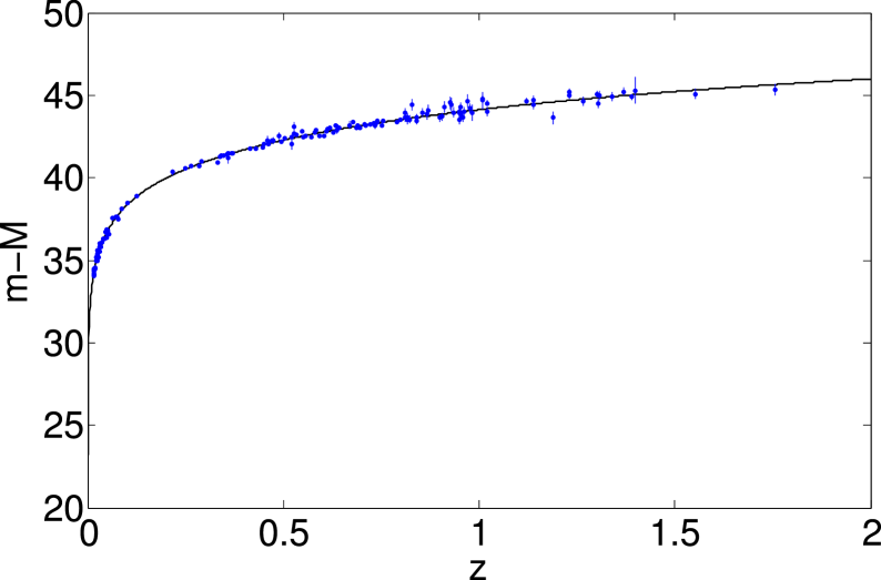
Fig. 1 : Solid line: supernova distance modulus, $\mu$, in terms of the redshift, z, for the concordance model. Observational data from the supernova legacy survey (Astier et al., 2006) and from a high redshift Hubble space telescope sample (Riess et al., 2006) are also shown.

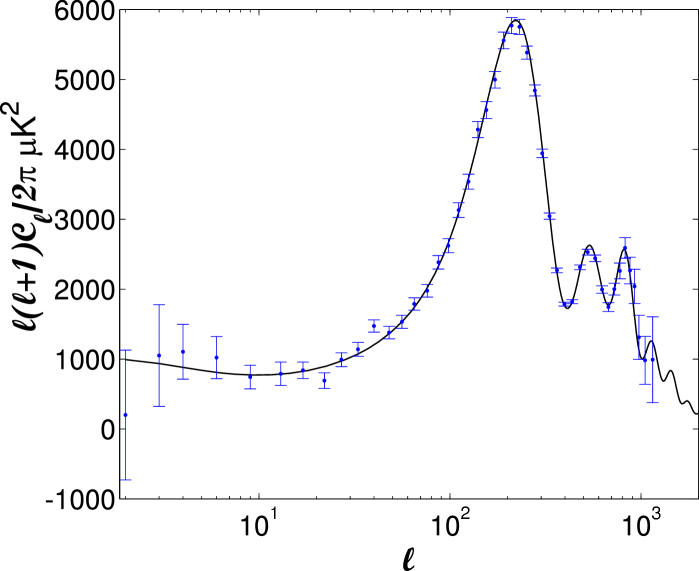
Fig. 2 : Solid line: CMB angular power spectrum for the concordance model including lensing. Observational data (WMAP seven years) and error bars (including cosmic variance) are also shown.

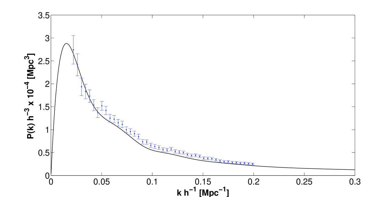
Fig. 3 : Solid line: all matter power spectrum estimated with CAMB for the concordance model. Observational data from the SDSS are also shown.

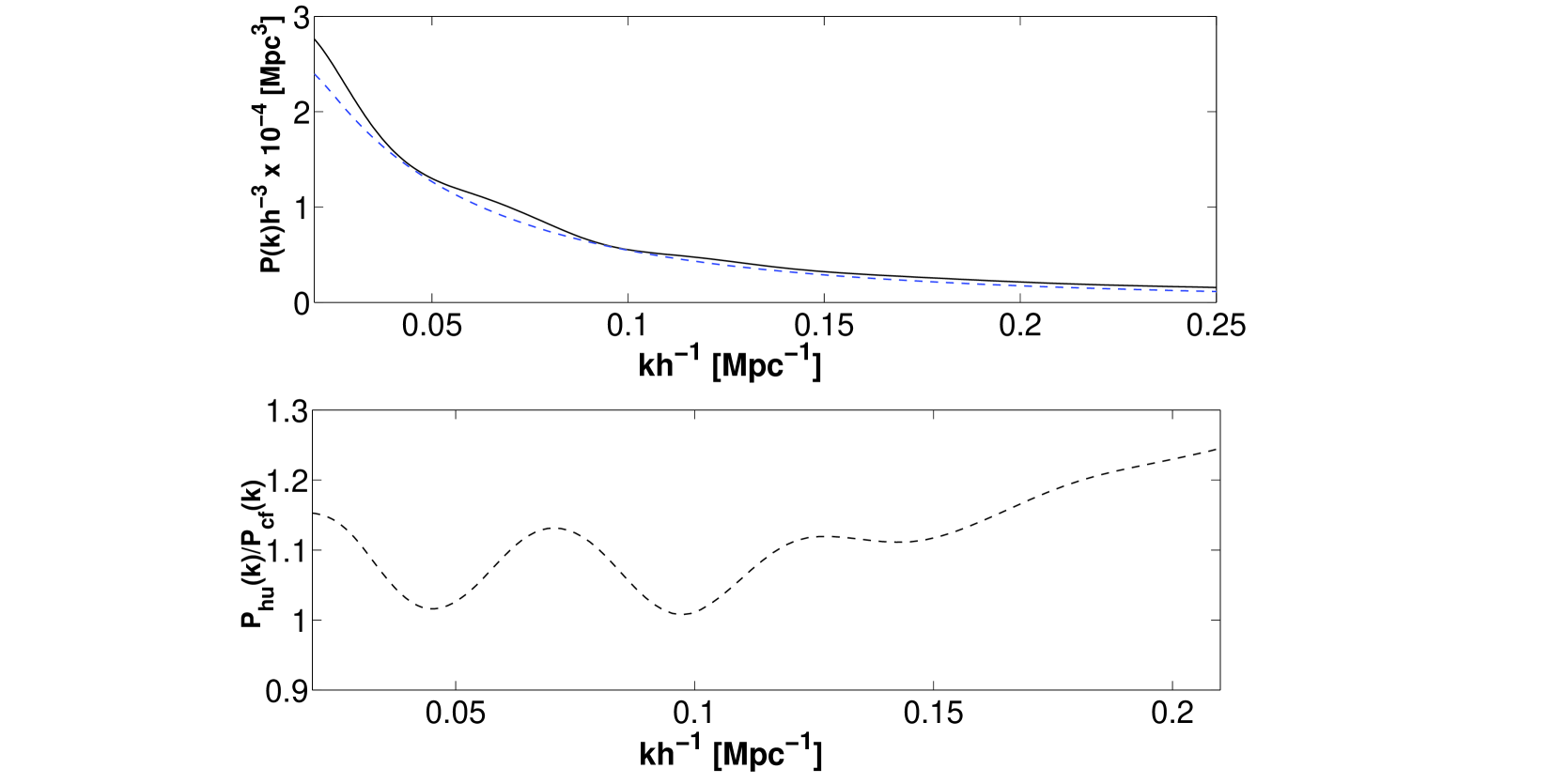
Fig. 4 : Top: Power spectrum of the matter energy density perturbations in the concordance model. Solid line is the true power spectrum estimated with CAMB. Dashed line shows the power spectrum –for the same model– in the absence of baryon acoustic oscillations. Bottom: Ratio between the power spectra showed in the to panel

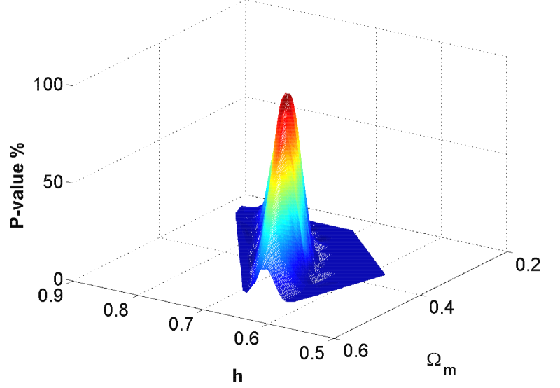
Fig. 5 : 3D representation of quantity $100p$ v.s. parameters $\Omega_{m}$ and $h$ for Ia SNe. Gravitation is described by the vector tensor theory of section 2

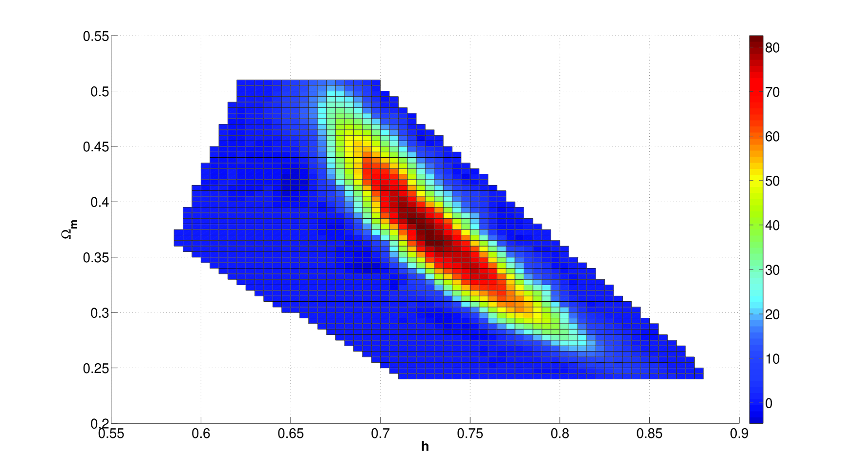
Fig. 6 : Projection of Fig. 5 on the ($\Omega_{m}$, $h$) plane. The color bar defines the $100p$ values in this 2D representation.

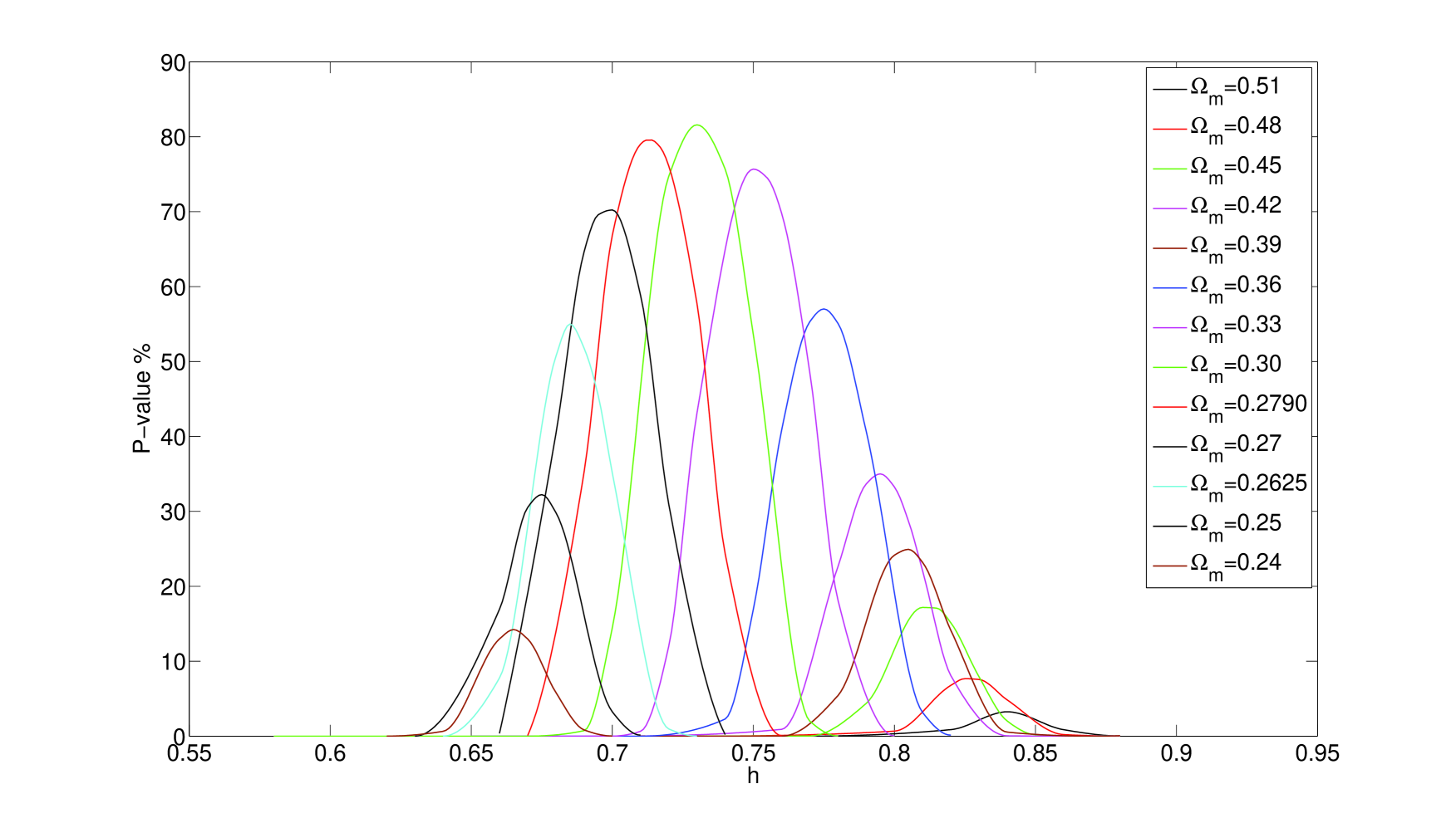
Fig. 7 : Quantity $100p$ v.s. $h$ for various $\Omega_{m}$ values. Each curve corresponds to an $\Omega_{m}$ value as it is displayed inside the panel.

Fig. 8 : Left: angular power spectrum of the CMB temperature for some parameter configurations of Table 1. Right: power spectrum of matter fluctuations for the same cases as in the corresponding left panels. The configurations considered in each level are: GR1 (solid), VT1 (dotted), and VT2 (dashed), in the panels of the top level; GR1 (solid), VT10 (dotted), and VT11(dashed) for the middle level; and GR1 (solid), VT13 (dotted), and VT14 (dashed) for the bottom panels.

Fig. 9 : Same as in Fig. 8 for the following configurations: GR1 (solid), VT3 (dashed) and VT4 (dotted) in the top level, GR1 (solid), VT4 (dotted), VT5 (dashed), and VT6 (dotted-dashed) in the panels of the middle level, and GR1 (solid), VT6 (dotted-dashed) , VT7 (dotted), and VT8 (dashed) in the bottom panels. In the bottom right panel cases VT6, VT7 and VT8 are indistinguishable.

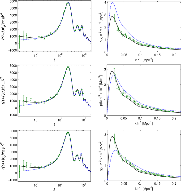
Fig. 10 : Same as in Fig. 8 for the following configurations: GR1 (solid) and VT9 (dotted) in the top panels, GR1 (solid) and VT12 (dotted) in the middle level, and GR1 (solid) and VT15 (dotted) in the panels of the bottom level. In this figure, the same observational data as in Figs. 2 and 3 have been also displayed in the left and right panels, respectively.

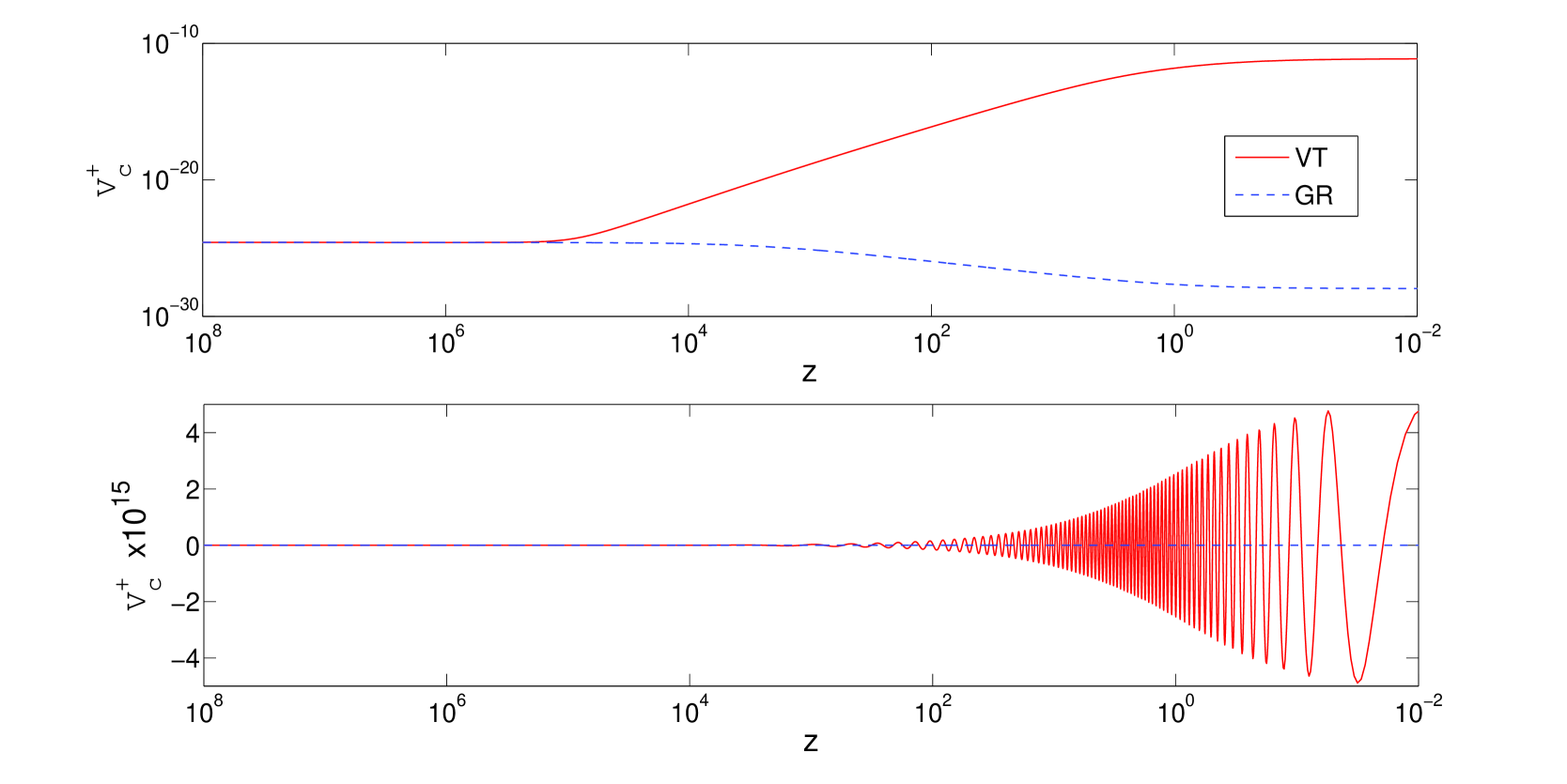
Fig. 11 : Time evolution of the gauge invariant quantity $v_{c}^{+}$ in the VT theory. Top (bottom) panel corresponds to a superhorizon (subhorizon) scale whose comoving length is $2\times 10^{4}\ Mpc$ ($2\times 10^{2}\ Mpc$). In both panels, the solid (dashed) line shows the VT (GR) evolution.

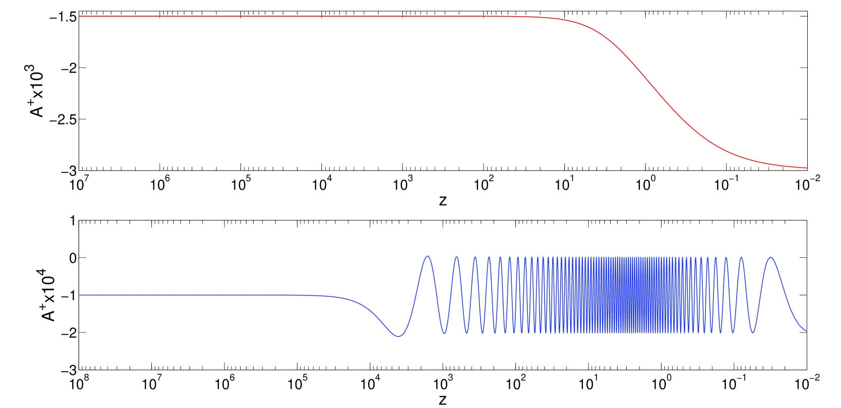
Fig. 12 : Same as in Fig. 11 for the gauge invariant quantity $A^{+}$

Acknowledgements This work has been supported by the Spanish Ministerio de Ciencia e Innovación, MICINN-FEDER project FIS2009-07705. We thank J.A. Morales-LLadosa and J. Benavent for useful discussion.

References

- Morales & Sáez (2007) Morales, J.A., & Sáez, D., Phys. Rev. D, 2007, 75, 043011
- Morales & Sáez (2008) Morales, J.A., & Sáez, D., Astrophys. J., 2008, 678, 503
- Dale, Morales & Sáez (2009) Dale, R., Morales, J.A., & Sáez, D., Physics and Mathematics of Gravitation, Proceedings of the Spanish Relativity Meeting 2008, AIP Conference Proceeding, 2009, 1122, 121
- Komatsu, et al. (2010) Komatsu, E. et al., arXiv:1001.4538[astro-ph]
- Larson, et al. (2010) Larson, D. et al., arXiv:1001.4635[astro-ph]
- Jarosik, et al. (2010) Jarosik, N. et al., arXiv:1001.4744[astro-ph]
- Reichardt, et al. (2008) Reichardt, C.L. et al., arXiv:0801.1491[astro-ph]
- Fowler et al. (2010) Fowler, J.W. et al., arXiv:1001.2934[astro-ph]
- Lueker et al. (2009) Lueker, M. et al., arXiv:0912.4317[astro-ph]
- Astier et al. (2006) Astier, P. et al., Astron. Astrophys., 2006, 447, 31
- Riess et al. (2006) Riess, A.G. et al., arXiv:0611572[astro-ph]
- Kowalski et al. (2008) Kowalski, M. et al., Astrophys. J., 2008, 686, 749
- Foley et al. (2009) Foley R.J. et al., Astron. J., 2009, 137, 3731
- Reid et al. (2009) Reid, B.A. et al., arXiv:0907.1659[astro-ph]
- Eisenstein et al. (2005) Eisenstein D.J. et al., Astrophys. J., 2005, 633, 560
- Takahashi (2009) Takahashi, R., Astrophys. J., 700, 479
- Martínez, et al. (2009) Martínez, V.J. et al., Astrophys. J. Lett., 2009, 696, 93
- Percival et al. (2009) Percival, W.J. et al., arXiv:0907.1660[astro-ph]
- Suyu et al. (2010) Suyu, H.H. et al., Astrophys. J., 2010, 711, 201
- Pettini et al. (2008) Pettini, M. et al., Mon. Not. R. Astron. Soc., 2008, 391, 1499
- Will (1993) Will, C.M., Theory and experiment in gravitational physics, Cambridge University Press, Cambridge, 1993
- Will (2006) Will, C.M., Living Rev. Relativity, 2006, 9, 3
- Zuntz, Ferreira & Zlosnik (2008) Zuntz, J.A., Ferreira, P.G., & Zlosnik, T.G., Phys. Rev. Lett., 2008, 101, 261102
- Böhmer & Harko (2007) Böhmer, C.G., & Harko, T., Eur. Phys. J. C., 2007, 50, 423
- Beltrán Jiménez & Maroto (2008) Beltrán Jiménez, J., & Maroto, A.L., Phys. Rev. D, 2008, 78, 063005
- Beltrán Jiménez, Lazkoz & Maroto (2009) Beltrán Jiménez, J., Lazkoz, R., & Maroto, A.L., Phys. Rev. D, 2009, 80, 023004
- Tartaglia & Radicella (2007) Tartaglia, A., & Radicella, N., Phys. Rev. D, 2007, 76, 083501
- Moffat (2006) Moffat, J.W., J. Cosmol. Astropart. Phys., 2006, JCAP 03/004, 001
- Lewis, Challinor & Lasenby (2000) Lewis, A., Challinor A., & Lasenby, A. Astrophys. J., 2000, 538, 473
- Hu & Eisenstein (1998) Hu, W., & Eisenstein, D.J., Astrophys. J., 1998, 498, 497
- Eisenstein & Hu (1998) Eisenstein, D.J., & Hu, W., Astrophys. J., 1998, 496, 605
- Becker et al. (2001) Becker R.H. et al., Astron. J., 2001, 122, 2850
- Page et al. (2007) Page, L. et al., Astrophys. J. Suppl. Ser., 2007, 170, 335
- Mukhanov & Vikman (2006) Mukhanov, V., & Vikman, A., J. Cosmol. Astropart. Phys., 2006, JCAP02/004, 001
- Bardeen (1980) Bardeen, J.M., Phys. Rev. D, 1980, 22, 1882
- Hu & White (1997) Hu, W., & White, M., Phys. Rev. D, 1997, 56, 596
- Ma & Bertschinger (1995) Ma, C.P., & Bertschinger, E., Astrophys. J., 1995, 455, 7