Aging of a Homogeneously Quenched Colloidal Glass-forming Liquid

Abstract

The non-equilibrium self-consistent generalized Langevin equation theory of colloid dynamics is used to describe the non-stationary aging processes occurring in a suddenly quenched model colloidal liquid with hard-sphere plus short-ranged attractive interactions, whose static structure factor and van Hove function evolve irreversibly from the initial conditions before the quench to a final, dynamically arrested state. The comparison of our numerical results with available simulation data are highly encouraging.

I Introduction.

The non-stationary, slowly-evolving dynamics of deeply quenched fluids, referred to as aging, has been the subject of considerable attention over the last decade cipelletti1 ; leheny1 . Concentrated emulsions emulsions , colloidal gels colloidalgels , and aqueous clay suspensions clays are some examples of aging systems. In spite of the apparent diversity of these structurally-disordered and out-of-equilibrium materials, the appearance of certain universal features in their non-equilibrium evolution suggests the existence of an underlying common source of the observed dynamic properties. Although this non-stationary behavior is associated with the formation of disordered solids, including hard materials such as polymer glasses polymerglasses , the main features are best exhibited by soft materials such as those above. In particular, the study of the dynamic properties of aging colloidal glasses and gels is specially interesting, since the observations provided, for example, by experimental methods such as dynamic light scattering vanmegenmortensen ; pham1 ; elmasriaging ; martinezvanmegen can sometimes be complemented with direct visualizations at the level of individual particles by means of digital video imaging techniques sanz1 ; lu1 . Computer simulation experiments in well-defined model systems have also contributed with important complementary information about the general properties of aging kobbarrat ; foffiaging1 ; puertas1 .

From the theoretical side the study of aging has been addressed in the field of spin glasses, where a mean-field theory has been developed within the last two decades cugliandolo1 . The models involved, however, lack a geometric structure and hence cannot describe the spatial evolution of real colloidal glass formers. About a decade ago Latz latz attempted to extend the mode coupling theory (MCT) of the ideal glass transition goetze1 ; goetze2 to describe the irreversible relaxation, including aging processes, of a suddenly quenched glass forming system. Similarly, De Gregorio et al. degregorio discussed time-translational invariance and the fluctuation-dissipation theorem in the context of the description of slow dynamics in system out of equilibrium but close to dynamical arrest. Unfortunately, in neither of these two theoretical efforts quantitative predictions were presented that could be contrasted with experimental or simulated results in specific model systems of structural glass-formers.

For concreteness, let us focus our discussion on the conceptually simplest glass-forming system, namely, a mono-component fluid made of $N$ identical spherical particles in a volume $V$ which interact through the pair potential $u(r)$ (although in the experimental realization of this idealized model we probably have to consider a small amount of polydispersity to suppress the kinetic pathway to ordered phases). Assume that in the absence of external fields this system is initially prepared in an equilibrium state corresponding to a mean density $\overline{n}^{(0)}=N/V$ and a temperature $T^{(0)}$, in which the static structure factor is $S^{(0)}(k)=S^{eq}(k;n,T^{(0)})$. In the simplest idealized quench experiment, at the time $t=0$ the temperature of the system is instantaneously and discontinuously changed to a value $T^{(f)}$. Let us assume that along the process that follows the quench, the density and the temperature are constrained to remain uniform and constant, i.e., that $\overline{n}(\textbf{r},t)=\overline{n}^{(0)}$ and $T(\textbf{r},t)=T^{(f)}$ at any position r in the volume $V$ and any time $t>0$. The relevant question then refers to the value of the static structure factor $S(k;t)$ for $t>0$, and to the evolution of the dynamic properties of the system along this process.

The referred dynamic properties can be described in terms of the relaxation of the fluctuations $\delta n({\bf r},t)$ of the local concentration $n({\bf r},t)$ of colloidal particles around its bulk equilibrium value $n$. The average decay of $\delta n({\bf r},t)$ is described by the two-time correlation function $F(k,\tau;t)\equiv N^{-1}\overline{\delta n({\bf k},t+\tau)\delta n(-{\bf k},t)}$ of the Fourier transform $\delta n({\bf k},t)$ of the fluctuations $\delta n({\bf r},t)$, whose equal-time limit is $S(k;t)\equiv F(k,\tau=0;t)=N^{-1}\overline{\delta n({\bf k},t)\delta n(-{\bf k},t)}$. We refer to the time $\tau$ as the correlation time, and the overline refers to the average over the probability distribution of the non-equilibrium ensemble that governs the statistical properties of $\delta n({\bf r},t)$ at the evolution time $t$. This ensemble will surely coincide with an equilibrium ensemble only in the limit $t\to\infty$, provided that no dynamic arrest condition appears along the process.

After the sudden temperature change at $t=0$ has occurred the system evolves spontaneously, searching for its new thermodynamic equilibrium state, at which the static structure factor should be $S^{eq}(k;n^{(0)},T^{(f)})$. If the end state, however, is a dynamically-arrested state (a glass or a gel), the system may never be able to reach this equilibrium state within experimental times; one then refers to the evolution time $t$ as the waiting or aging time pham1 ; cipelletti1 ; martinezvanmegen ; sanz1 ; lu1 . The dependence of $S(k;t)$ and $F(k,\tau;t)$ on $t$ characterizes the non-equilibrium evolution of the system, whose quantitative theoretical first-principles description, to our knowledge, has not been available until now, in spite of important theoretical efforts like those referred to above.

In recent related work nescgle1 , however, an extension was proposed of the self-consistent generalized Langevin equation (SCGLE) theory of colloid dynamics scgle0 ; scgle1 ; scgle2 ; marco1 ; marco2 and dynamic arrest rmf ; todos1 ; todos2 ; attractive1 ; soft1 ; rigo1 ; rigo2 ; luis1 , aimed precisely at describing this non-equilibrium evolution of $S(k;t)$ and $F(k,\tau;t)$. This extension was based on Onsager’s theory of thermal fluctuations onsager1 ; onsager2 ; onsagermachlup1 ; onsagermachlup2 ; keizer , adequately extended delrio ; faraday to allow for the description of memory effects. The purpose of the present paper is to provide the first practical and concrete application of such general non-equilibrium theory of colloid dynamics by means of its use in the quantitative description of the aging process of a model monocomponent glass-forming liquid.

In this particular context, such non-equilibrium self-consistent generalized Langevin equation (NE-SCGLE) theory consists of a closed self-consistent system of equations for $S(k;t)$ and $F(k,\tau;t)$, which we numerically solve here for a model mono-component fluid of particles interacting through the hard-sphere plus short-ranged attractive Yukawa potential. This model system exhibits the glass-fluid-glass reentrance predicted by the equilibrium SCGLE theory attractive1 (and originally discovered by MCT bergenholtz1 ). Here we discuss the isochoric quench of this fluid from an initial equilibrium state ($n^{(0)},T^{(0)}$) in the reentrant fluid pocket of the ($n,T$) state space, to a final temperature $T^{(f)}\ (<T^{(0)})$ in the vicinity and below the attractive glass transition temperature $T^{(a)}(n^{(0)})$ corresponding to the density $n^{(0)}$. This process mimics the computer simulation aging experiment reported by Foffi et al. foffiaging1 in a similar model system (hard-sphere plus short-ranged square well). Here we discuss our theoretical predictions in reference to the observed behavior in this simulated quench experiment.

We start this discussion by summarizing in the following section the full non-equilibrium self-consistent generalized Langevin equation (NE-SCGLE) theory, which does not involve the restrictive assumption of spatial homogeneity. In the same section this theory is simplified according to the assumption that the system is constrained to remain spatially homogeneous and isotropic. The actual solution of the resulting equations are reported in Sec. III. The last section contains a summary of the results.

II non-equilibrium self-consistent generalized Langevin equation theory

The previous discussion implicitly assumes that $S(k;t)$ and $F(k,\tau;t)$ adequately represent the structural and dynamic properties of the quenched system along the irreversible equilibration process. This assumption, which is thought to be accurate in the absence of external fields, or when the effects of these external fields are very small, is in reality a strong simplifying assumption when the local concentration fluctuations do not relax within experimental times, as it occurs at and near dynamically arrested states. The general non-equilibrium SCGLE theory proposed in ref. nescgle1 , however, does not incorporate this simplifying assumption at the outset. Instead, it describes the statistical properties of the instantaneous local concentration profile $n(\textbf{r},t)$ of the colloidal liquid in terms of the coupled time evolution equations for its mean value $\overline{n}(\textbf{r},t)$ and for the covariance $\sigma(\textbf{r},\textbf{r}^{\prime};t)\equiv\overline{\delta n(\textbf{r},t)\delta n(\textbf{r}^{\prime},t)}$ of the fluctuations $\delta n(\textbf{r},t)=n(\textbf{r},t)-\overline{n}(\textbf{r},t)$. In this section we briefly review the general NE-SCGLE theory and then particularize it to instantaneous homogeneous quench processes.

II.1 General NE-SCGLE theory.

The referred equations for $n(\textbf{r},t)$ and $\sigma(\textbf{r},\textbf{r}^{\prime};t)$ read nescgle1

$$\frac{\partial\overline{n}(\textbf{r},t)}{\partial t}=D^{0}{\nabla}\cdot b(\textbf{r},t)\overline{n}(\textbf{r},t)\nabla\beta\mu[{\bf r};\overline{n}(t)]$$ (1)

and

$$\begin{split}\frac{\partial\sigma(\textbf{r},\textbf{r}^{\prime};t)}{\partial t}=&D^{0}{\nabla}\cdot\overline{n}(\textbf{r},t)\ b(\textbf{r},t)\nabla\int d\textbf{r}_{1}\mathcal{E}[\textbf{r},\textbf{r}_{1};\overline{n}(t)]\sigma(\textbf{r}_{1},\textbf{r}^{\prime};t)\\ &+D^{0}{\nabla}^{\prime}\cdot\overline{n}(\textbf{r}^{\prime},t)\ b(\textbf{r}^{\prime},t)\nabla^{\prime}\int d\textbf{r}_{1}\mathcal{E}[\textbf{r}^{\prime},\textbf{r}_{1};\overline{n}(t)]\sigma(\textbf{r}_{1},\textbf{r};t)\\ &-2D^{0}{\nabla}\cdot\overline{n}(\textbf{r},t)\ b(\textbf{r},t)\nabla\delta(\textbf{r}-\textbf{r}^{\prime}),\end{split}$$ (2)

in which $D_{0}$ is the self-diffusion coefficient of the colloidal particles in the absence of direct interactions, $\mu[{\bf r};n]$ is the electrochemical potential at position r (which is a functional of the local concentration profile $n(\textbf{r})$), and $\mathcal{E}[\textbf{r},\textbf{r}^{\prime};\overline{n}(t)]$ is the functional derivative $\mathcal{E}[\textbf{r},\textbf{r}^{\prime};n]\equiv\left[{\delta\beta\mu[{\bf r};n]}/{\delta n({\bf r}^{\prime})}\right]$ evaluated at the concentration profile $n(\textbf{r})=\overline{n}(\textbf{r},t)$. Thus, for given $D_{0}$ and $\mu[{\bf r};n]$, Eqs. (1) and (2) would constitute a closed system of equations for $\overline{n}(\textbf{r},t)$ and $\sigma(\textbf{r},\textbf{r}^{\prime};t)$ if it were not for the presence of the dimensionless local mobility function $b(\textbf{r},t)$.

This mobility function $b(\textbf{r},t)$ describes the local frictional effects of the direct (i.e., conservative) interactions between the colloidal particles, as deviations from the value $b(\textbf{r},t)=1$, and can be expressed in terms of the memory function of the two-time correlation function $C^{(2)}(\textbf{r},\textbf{r}^{\prime};t,t^{\prime})\equiv\overline{\delta n(\textbf{r},t)\delta n(\textbf{r}^{\prime},t^{\prime})}$, which we write as $C^{(2)}(\textbf{r},\textbf{r}+\textbf{x};t,t+\tau)\equiv C(\textbf{x},\tau;\textbf{r},t)$, and which is the value of the van Hove function at a spatial location r in the system and at an evolution time $t$. Since the covariance is $\sigma(\textbf{r},\textbf{r}^{\prime};t)=C^{(2)}(\textbf{r},\textbf{r}^{\prime};t,t)=C(\textbf{x},\tau=0;\textbf{r},t)$, it can also be written as $\sigma(\textbf{x};\textbf{r},t)$. Although in the development of the non-equilibrium SCGLE theory the assumption of absolute spatial homogeneity and isotropy is avoided, these spatially-varying van Hove function and covariance do depend on the location r in space but are assumed to be approximately isotropic within a small volume around r, so that they only depend on the magnitude $|\textbf{x}|$ of the correlation vector x. Under these conditions, the local covariance $\sigma(|\textbf{x}|;\textbf{r},t)$ can be written in terms of its Fourier transform $\sigma(k;\textbf{r},t)$ as

$$\sigma(\mid\textbf{x}\mid;\textbf{r},t)=\frac{1}{(2\pi)^{3}}\int d^{3}ke^{-i\textbf{k}\cdot\textbf{x}}\sigma(k;\textbf{r},t),$$ (3)

so that Eq. (2) may be re-written as

$$\begin{split}\frac{\partial\sigma(k;\textbf{r},t)}{\partial t}=&-2k^{2}D^{0}\overline{n}(\textbf{r},t)b(\textbf{r},t)\mathcal{E}(k;\overline{n}(\textbf{r},t))\sigma(k;\textbf{r},t)\\ &+2k^{2}D^{0}\overline{n}(\textbf{r},t)\ b(\textbf{r},t),\end{split}$$ (4)

where $\mathcal{E}(k;\overline{n}(\textbf{r},t))\equiv(2\pi)^{-3}\int d^{3}ke^{-i\textbf{k}\cdot\textbf{x}}\mathcal{E}[\textbf{r},\textbf{r}+\textbf{x};\overline{n}(\textbf{r},t)]$. Similarly, the local van Hove function $C(|\textbf{x}|,\tau;\textbf{r},t)$ can also be expressed in terms of its spatial Fourier transform as

$$C(\mid\textbf{x}\mid,\tau;\textbf{r},t)=\frac{1}{(2\pi)^{3}}\int d^{3}ke^{-i\textbf{k}\cdot\textbf{x}}C(k,\tau;\textbf{r},t).$$ (5)

Let us notice that we can also introduce the notation $C(k,\tau;\textbf{r},t)=\overline{n}(\textbf{r},t)F(k,\tau;\textbf{r},t)$, with $F(k,\tau;\textbf{r},t)$ being the non-equilibrium intermediate scattering function, whose initial value $F(k,\tau=0;\textbf{r},t)=S(k;\textbf{r},t)$ defines the time-evolving spatially-varying static structure factor $S(k;\textbf{r},t)$; this more familiar notation will be employed later on.

According to Ref. nescgle1 , the actual calculation of the local mobility function $b(\textbf{r},t)$ requires the solution, at each position r and each evolution time $t$, of a system of equations involving the Laplace transform (LT) of $C(k,\tau;\textbf{r},t)$ (denoted by $\hat{C}(k,z;\textbf{r},t)\equiv\int_{0}^{\infty}d\tau e^{-z\tau}C(k,\tau;\textbf{r},t)$), as well as the LT of its self component $C_{S}(k,\tau;\textbf{r},t)$, and of the $\tau$-dependent friction function $\Delta\zeta^{*}(\tau;\textbf{r},t)$, namely,

$$\hat{C}(k,z;\textbf{r},t)=\frac{\sigma(k;\textbf{r},t)}{z+\frac{k^{2}D^{0}\overline{n}(\textbf{r},t)\sigma^{-1}(k;\textbf{r},t)}{1+\lambda(k)\ \Delta\hat{\zeta}^{*}(z;\textbf{r},t)}},$$ (6)

$$\hat{C}_{S}(k,z;\textbf{r},t)=\frac{1}{z+\frac{k^{2}D^{0}}{1+\lambda(k)\ \Delta\hat{\zeta}^{*}(z;\textbf{r},t)}},$$ (7)

and

$$\Delta\zeta^{*}(\tau;\textbf{r},t)=\frac{D_{0}}{3\left(2\pi\right)^{3}}\int d{\bf k}\ k^{2}\left[\frac{\sigma(k;\textbf{r},t)/\overline{n}(\textbf{r},t)-1}{\sigma(k;\textbf{r},t)}\right]^{2}C(k,\tau;\textbf{r},t)C_{S}(k,\tau;\textbf{r},t).$$ (8)

with $\lambda(k)$ being a phenomenological “interpolating function” given by nescgle1 ; todos1 ; todos2

$$\lambda(k)=\frac{1}{1+\left(\frac{k}{k_{c}}\right)^{2}},$$ (9)

where $k_{c}\gtrsim 2\pi/d$, with $d$ being some form of distance of closest approach. A simple empirical prescription is to choose $k_{c}$ as $k_{c}=k_{\min}$, the position of the first minimum (beyond the main peak) of the static structure factor $S(k;\textbf{r},t)=\sigma(k;\textbf{r},t)/\overline{n}(\textbf{r},t)$. The local mobility $b(\textbf{r},t)$ finally follows from the solution of these equations by means of its relation with $\Delta\hat{\zeta}^{*}(z;\textbf{r},t)$, namely,

$$b(\textbf{r},t)=\left[1+\Delta\hat{\zeta}^{*}(z=0;\textbf{r},t)\right]^{-1}.$$ (10)

II.2 Instantaneous homogeneous quench.

Let us now discuss the application of this general theory to the particular conditions referring to the irreversible evolution of the structure and dynamics of a system constrained to suffer a programmed process of homogeneous compression or expansion (and/or of cooling or heating). Under these conditions, rather than solving Eq. (1) for $\overline{n}({\bf r};t)$, we assume that the system is constrained to remain spatially uniform, $\overline{n}({\bf r};t)=\overline{n}(t)$, according to a prescribed time-dependence $\overline{n}(t)$ of the uniform bulk concentration (and/or to a prescribed uniform time-dependent temperature $T(t)$). In consistency with this assumed constraint we have that the dependence on the position r disappears from the previous equations so that, for example, Eq. (4) may be re-written as

$$\frac{\partial\sigma(k;t)}{\partial t}=-2k^{2}D^{0}\overline{n}(t)b(t)\mathcal{E}(k;t)\left[\sigma(k;t)-\mathcal{E}^{-1}(k;t)\right],$$ (11)

with $\mathcal{E}(k;t)\equiv\mathcal{E}(k;\overline{n}(t))$ and with

$$b(t)=\left[1+\int_{0}^{\infty}d\tau\Delta{\zeta}^{*}(\tau;t)\right]^{-1},$$ (12)

where $\Delta{\zeta}^{*}(\tau;t)$ is provided by the solution of the self-consistent system in Eqs. (6)-(8) for the uniform bulk concentration $\overline{n}({\bf r};t)=\overline{n}(t)$.

Among the many possible programmed protocols ($\overline{n}(t)$, $T(t)$) that one could devise to drive or to prepare the system, the simplest corresponds to the idealized quasi-static process, in which the relaxation rate $\partial\sigma(k;t)/\partial t$ is virtually negligible due to a virtually instantaneous “thermalization” of $\sigma(k;t)$ to its local equilibrium value $\sigma^{l.e.}(k;t)\equiv 1/\mathcal{E}(k;t)$ nescgle1 ; keizer . A quasi-static process, however, is a rather unrealistic concept, at least in the limit of small wave-vectors, in which the relaxation times diverge as $k^{-2}$, as seen in the example below. In contrast, a far more interesting and fundamental protocol corresponds to the opposite limit, in which the system, initially at an equilibrium state determined by initial values of the control parameters, $(\overline{n}^{(0)},T^{(0)})$, must adjust itself in response to a sudden and instantaneous change of these control parameters to new values $(\overline{n}^{(f)},T^{(f)})$, according to the “program” $\overline{n}(t)=\overline{n}^{(0)}\theta(-t)+\overline{n}^{(f)}\theta(t)$ and $T(t)=T^{(0)}\theta(-t)+T^{(f)}\theta(t)$, with $\theta(t)$ being Heavyside’s step function.

Under these conditions the formal solution of Eq. (11) can be written, for $t>0$, as

$$\sigma(k;t)=\sigma^{0}(k)e^{-\alpha(k)u(t)}+[\mathcal{E}^{(f)}(k)]^{-1}\left(1-e^{-\alpha(k)u(t)}\right),$$ (13)

where $\mathcal{E}^{(f)}(k)=\mathcal{E}(k;\overline{n}^{(f)},T^{(f)})$ is the Fourier transform of $\mathcal{E}[\mid\textbf{r}-\textbf{r}^{\prime}\mid;\overline{n}^{(f)},T^{(f)}]\equiv\left[{\delta\beta\mu[{\bf r};n]}/{\delta n({\bf r}^{\prime})}\right]_{n=\overline{n}^{(f)},T=T^{(f)}}$,

$$u(t)\equiv\int_{0}^{t}b(t^{\prime})dt^{\prime},$$ (14)

and

$$\alpha(k)\equiv 2k^{2}D^{0}\bar{n}^{(f)}\mathcal{E}^{(f)}(k).$$ (15)

Clearly, the presence of the time-dependent mobility $b(t)$ couples this formal solution with the self-consistent system in Eqs. (6)-(8). For the present conditions, and in terms of the non-stationary static structure factor $S(k;t)\equiv\sigma(k;t)/\overline{n}^{(f)}$ and intermediate scattering function $F(k,\tau;t)\equiv C(k,\tau;t)/\overline{n}^{(f)}$, we may rewrite such self-consistent system of equations as

$$\hat{F}(k,z;t)=\frac{S(k;t)}{z+\frac{k^{2}D^{0}S^{-1}(k;t)}{1+\lambda(k)\ \Delta\hat{\zeta}^{*}(z;t)}},$$ (16)

$$\hat{F}_{S}(k,z;t)=\frac{1}{z+\frac{k^{2}D^{0}}{1+\lambda(k)\ \Delta\hat{\zeta}^{*}(z;t)}},$$ (17)

and

$$\Delta\zeta^{*}(\tau;t)=\frac{D_{0}}{3\left(2\pi\right)^{3}\overline{n}^{(f)}}\int d{\bf k}\ k^{2}\left[\frac{S(k;t)-1}{S(k;t)}\right]^{2}F(k,\tau;t)F_{S}(k,\tau;t).$$ (18)

Eqs. (12)-(18) constitute our general self-consistent description of the spontaneous evolution of the structure and dynamics of an instantaneously and homogeneously quenched liquid.

Of course, one important aspect of this analysis refers to the possibility that the end state of the quench process happens to be in the region of dynamically arrested states. For the discussion of this important aspect it is useful to consider the long-$\tau$ (or small $z$) asymptotic stationary solutions of Eqs. (16)-(18) above. Just like in the equilibrium SCGLE theory todos1 , these may be analyzed in terms of the asymptotic values of these dynamic properties (the so-called non-ergodicity parameters), given by nescgle1

$$f(k;t)\equiv\lim_{\tau\to\infty}\frac{F(k,\tau;t)}{S(k)}=\frac{\lambda(k;t)S(k;t)}{\lambda(k;t)S(k;t)+k^{2}\gamma(t)}$$ (19)

and

$$f_{S}(k;t)\equiv\lim_{\tau\to\infty}F_{S}(k,\tau;t)=\frac{\lambda(k;t)}{\lambda(k;t)+k^{2}\gamma(t)},$$ (20)

where the squared localization length $\gamma(t)$ is the solution of

$$\frac{1}{\gamma(t)}=\frac{1}{6\pi^{2}\overline{n}^{(f)}}\int_{0}^{\infty}dkk^{4}\frac{\left[S(k;t)-1\right]^{2}\lambda^{2}(k;t)}{\left[\lambda(k;t)S(k;t)+k^{2}\gamma(t)\right]\left[\lambda(k;t)+k^{2}\gamma(t)\right]}.$$ (21)

These equations are the non-equilibrium extension of the corresponding results of the equilibrium SCGLE theory, and their derivation from Eqs. (16)-(18) follows the same arguments as in the equilibrium case scgle2 .

In the following section we numerically solve Eqs. (12)-(18) for still more specific conditions, namely, for an isochoric quench of a model colloidal system, in which $\overline{n}^{(f)}=\overline{n}^{(0)}$ and Eq. (13) can be written in terms of the time-evolving static structure factor $S(k;t)=\sigma(k;t)/\overline{n}^{(f)}$ as

$$S(k;t)=S^{0}(k)e^{-\alpha(k)u(t)}+S^{eq}_{f}(k)\left(1-e^{-\alpha(k)u(t)}\right),$$ (22)

with $S^{eq}_{f}(k)\equiv[\overline{n}^{(f)}\mathcal{E}^{(f)}(k)]^{-1}$. Let us notice that in the limit in which the friction function $\Delta{\zeta}^{*}(\tau;t)$ vanishes, $b(t)=1$ and hence $u(t)=t$, so that Eq. (22) reads

$$S^{*}(k;t)=S^{0}(k)e^{-\alpha(k)t}+S^{eq}_{f}(k)\left(1-e^{-\alpha(k)t}\right).$$ (23)

This limiting expression describes an exponential interpolation of $S(k;t)$ between its initial value $S^{0}(k)$ and its final equilibrium value $S^{eq}_{f}(k)\equiv[\overline{n}^{(f)}\mathcal{E}^{(f)}(k)]^{-1}$. It is then important to notice that the general solution $S(k;t)$ in Eq. (22) can be written in terms of this particular solution as $S(k;t)=S^{*}(k;u(t))$, with $u(t)$ given by Eq. (14). This means that a sequence of static structure factors $S^{*}(k;u_{n})$ generated by this simple exponential interpolating formula when the time $t$ is given a sequence of values $u_{n}$, say $u_{n}=n\Delta u$ (with $n=0,1,2,...$), will be identical to the sequence $S(k;t_{n})$ generated when the exact solution in Eq. (22) is evaluated at a different sequence $t_{n}$ ($n=0,1,2,...)$, provided that the times $u_{n}$ and $t_{n}$ are related by $u_{n}=\int_{0}^{t_{n}}b(t^{\prime})dt^{\prime}$. This observation greatly simplifies the mathematical analysis and the numerical method of solution of the full self-consistent theory under the particular conditions considered here.

The solution ${\gamma(t)}$ of Eq. (21) provides a dynamic order parameter in the sense that when it is infinite we can say that at that waiting time $t$ the system remains ergodic, whereas if it is finite, we say that the system became dynamically arrested. A practical manner to use this criterion is to first construct a sequence of static structure factors $S^{*}(k;u_{n})$ using Eq. (23) for the uniform sequence $u_{n}=n\Delta u$ (with $n=0,1,2,...$). Each member of this sequence is then employed as the static input to solve self-consistently Eqs. (16)-(18), thus evaluating, using Eq. (12), a mobility sequence $b(u_{n})$. Since the sequence $S^{*}(k;u_{n})$ is identical to the sequence $S(k;t_{n})$ provided that $u_{n}=\int_{0}^{t_{n}}b(t^{\prime})dt^{\prime}$, the mobility $b(u_{n})$ must be identical to $b(t_{n})$, and the corresponding time-sequence $t_{n}$ can be determined by means of the approximate recursive relation $t_{n+1}=t_{n}+(\Delta u)/b(t_{n})$. If the dynamic arrest condition occurs along this process, i.e., if a value $u^{(a)}$ exists such that $\gamma(u)$ (determined using $S^{*}(k;u)$ in Eq. (21)) is infinite for $u<u^{(a)}$ and finite for $u>u^{(a)}$, then $b(u)\to 0$ when $u\to u^{(a)}$ from below, and it is then not difficult to realize that the corresponding dynamic arrest time $t^{(a)}$ will diverge and $u^{(a)}=\int_{0}^{\infty}b(t^{\prime})dt^{\prime}$. The following numerical results illustrate the physical implications of this singular behavior.

III Illustrative application.

Let us now apply the theory just presented, to a concrete model system, namely, a dispersion of colloidal particles interacting through the hard-sphere plus attractive Yukawa pair potential expressed, in units of the thermal energy $k_{B}T=\beta^{-1}$, as

$$\beta u(r)=\begin{cases}\infty,&r<\sigma_{HS};\\ -K\frac{\exp[-z(r/\sigma_{HS}-1)]}{(r/\sigma_{HS})},&r>\sigma_{HS}.\end{cases}$$ (24)

The state space of this system is spanned by the volume fraction $\phi=\pi\overline{n}\sigma_{HS}^{3}/6$ and the reduced temperature $T^{*}\equiv K^{-1}$, as illustrated in Fig. 1. The equilibrium phase diagram of this system includes the gas and liquid disordered phases and crystalline solid phases. Here we will describe the equilibrium static structure factor $S^{eq}(k;\phi,T^{*})=[\overline{n}\mathcal{E}^{eq}(k;\overline{n},T^{*})]^{-1}$ of the disordered phases within the mean spherical approximation (MSA) hoyeblum . Using this approximation and the compressibility equation mcquarrie one can determine the spinodal curve of the gas-liquid transition by means of the condition $1/S^{eq}(k=0;\phi,T^{*})=0$; the result is plotted in Fig. 1 for $z=20$.

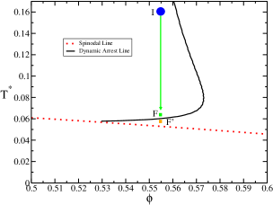
Figure 1: State space $(\phi,T^{*})$ of the hard-sphere plus attractive Yukawa model system ($z=20$). The dotted line is the spinodal curve and the solid line is the dynamic arrest line calculated using Eq. (21) within the mean spherical approximation (MSA) for the equilibrium static structure factor $S^{eq}(k;\phi,T^{*})$. We consider an instantaneous quench process at $t=0$ from the ergodic initial state $I$ to the final state $F$ near but slightly above the attractive glass “branch” of the dynamic arrest line. We also consider a second process, now to the point $F^{\prime}$ below this dynamic arrest line but still above the spinodal curve.

Using the same MSA equilibrium static structure factor $S^{eq}(k;\phi,T^{*})$ in the equilibrium version of Eq. (21) we can scan the state space $(\phi,T^{*})$ to determine $\gamma^{eq}$ at any point $(\phi,T^{*})$ attractive1 . In this manner one locates the dynamic arrest transition line indicated by the solid curve of Fig. 1. The region to the right and below this curve is thus predicted to correspond to dynamically arrested states. This figure focusses on the high-density glass-fluid-glass reentrance region that was first discovered using mode coupling theory bergenholtz1 . We now follow the approach introduced by Foffi et al. foffiaging1 in a simulation experiment on a very similar model system (a hard-sphere plus square-well fluid). Such experiment corresponds to suddenly quenching the system under isochoric conditions from an initial state $(\phi_{0},T^{*}_{I})$ located in the fluid pocket of the reentrance (point $I$ in Fig. 1), to a final state near the fluid-“attractive glass” transition line (either point $F$ or point $F^{\prime}$ in Fig 1). In the first case the end state $(\phi_{0},T^{*}_{F})$ lies slightly above the transition line, whereas in the second, the end state $(\phi_{0},T^{*}_{F^{\prime}})$ lies in the region of arrested states.

For this process we solve the general self-consistent system of equations in Eqs. (12)-(18). The specific calculations are performed along the isochore $\phi_{0}=0.555$ with initial temperature $T_{I}^{*}=0.159$ and final temperature $T^{*}_{F}=0.0604$. Fig. 2 illustrates the irreversible evolution of the static structure factor $S(k;t_{w})$ as a sequence of snapshots corresponding to five intermediate waiting times $t_{w}$ (from now on denoted by $t_{w}$, rather than simply by $t$). We observe that the structure, initially described by $S^{eq}(k;\phi_{0},T_{I}^{*})$, relaxes to the expected final value $S^{eq}(k;\phi_{0},T_{F}^{*})$, and that this process is faster at large wave-vectors, where it involves the appearance of stronger oscillations with $k$ and a general shift of the maxima of $S(k;t)$ to larger wave-vectors. To a large extent these features can be understood in terms even of the simple interpolating expression in Eq. (23).

Figure 2: Non-equilibrium evolution of the static structure factor $S(k,t_{w})$. The system, initially equilibrated at $(\phi_{0},T_{I}^{*})=(0.555,0.159)$, with $S(k;t=0)=S^{eq}(k;\phi_{0},T_{I}^{*})$ ((black) dotted curve), is instantaneously quenched at $t_{w}=0$ to the final point $(\phi_{0},T_{F}^{*})=(0.555,0.0604)$. The static structure factor then evolves continuously along a sequence of non-equilibrium values ((red) point-dashed lines) illustrated by the snapshots corresponding to $t_{w}/t_{0}=3.2,\ 60.87,\ 174.29,\ 945.39,\ 2023.54,\ \textrm{and}\ 4858.84$, with $t_{0}\equiv[\sigma^{2}/D_{0}]$. Since the point $F$ lies outside the dynamic arrest region, $S(k,t_{w})$ eventually attains its final equilibrium value $S(k;t_{w}=\infty)=S^{eq}(k;\phi_{0},T_{F}^{*})$ ((blue) dashed curve). The main figure shows the resulting relaxation process in a wide $k$-range and the inset zooms on the evolution of the main peak of $S(k,t_{w})$.

The corresponding adjustment of the main peak of $S(k;t_{w})$ from its initial value $S^{eq}(k_{max};\phi_{0},T^{*}_{I})$ to its final value $S^{eq}(k_{max};\phi_{0},T^{*}_{F})\ (<S^{eq}(k_{max};\phi_{0},T^{*}_{I}))$ occurs, however, notoriously more slowly than at large wave-vectors and in an apparently non-monotonic manner, as illustrated in the inset of Fig. 2, which zooms on the evolution of the main peak. As observed there, as the system evolves, the maximum of $S(k;t_{w})$ moves to the right while decreasing in height to a value smaller than $S^{eq}(k_{max};\phi_{0},T^{*}_{F})$, bouncing back at later times to reach this final value. The origin of the predicted non-monotonic behavior can also be understood on the basis of the simple interpolation expression in Eq. (23), which implies that $S(k;t)$ will not change with waiting time for the wave-vectors $k^{*}$ at which the initial and the final static structure factors are already identical, $S^{eq}(k^{*};\phi_{0},T^{*}_{I})=S^{eq}(k^{*};\phi_{0},T^{*}_{F})$. It is then not difficult to see that if the condition $k^{(I)}_{max}<k^{*}<k^{(F)}_{max}$ occurs, as it happens in our example, we shall observe this non-monotonic effect.

A more interesting effect, which is perceptible in Fig. 2, but which is illustrated in more detail in Fig 3, is the evolution of $S(k;t_{w})$ at smaller wave-vectors. This refers to the emergence of a non-equilibrium low-$k$ peak that indicates the appearance of spatial heterogeneities of average size $\lambda_{1}(t_{w})\approx 2\pi/k_{1}(t_{w})$, with $k_{1}$ being the position of this emerging low-$k$ maximum. Fig 3.a provides a zoom on this effect in the case of the slightly deeper quench, now to the final state point $F^{\prime}$ in Fig. 1, with temperature $T^{*}_{F^{\prime}}=0.0588$ slightly below the dynamic arrest line. These heterogeneities may be associated with the appearance of voids whose average size and importance increase with waiting time, as suggested by the increasing height of the peak and by its shift to smaller wave-vectors observed as the system evolves. The emergence of this peak is associated with the vicinity of the gas-liquid spinodal region. In fact, it has the same origin as the low-$k$ peak that characterizes the process of early spinodal decomposition cook , even though in our case the final state $(\phi_{0},T^{*}_{F^{\prime}})$ lies outside the spinodal region.

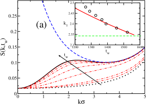
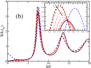
Figure 3: Non-equilibrium evolution of the static structure factor $S(k,t_{w})$ for the deeper quench to the final state point $F^{\prime}$. The system, initially equilibrated at $(\phi_{0},T_{I}^{*})=(0.555,0.159)$, with $S(k;t=0)=S^{eq}(k;\phi_{0},T_{I}^{*})$ ((black) dotted curve), is instantaneously quenched at $t_{w}=0$ to the final point$(\phi,T_{F^{\prime}})=(0.555,0.0588)$ inside the dynamic arrest region. The static structure factor then evolves continuously along a sequence of non-equilibrium values ((red) point-dashed lines) illustrated by the snapshots corresponding to $t_{w}/t_{0}=0.0,\ 1.23,\ 3.84,\ 140,\ 490,\ 975,\ 1265,$ and $1522$ ($\approx t_{w}^{(c)}/t_{0}$). Panel (a) focuses on the low-$k$ peak of $S(k,t_{w})$, and its inset shows the dependence of the position $k_{1}(t_{w})$ of this low-$k$ peak on the waiting time $t_{w}$ (empty circles), with the solid line being the fit of the last few points with $k_{1}(t_{w})\approx(t_{w})^{-\alpha}$ and $\alpha\approx\frac{1}{5}$. Panel (b) shows the behavior in a larger $k$-regime, similar to Fig. 2, with its inset zooming on the evolution of the main peak.

As said above, this phenomenon is already observed in the shallower quench of Fig. 2. In that case, however, although the system slows down considerably, the final structure of the irreversible evolution of $S(k;t_{w})$ is still the expected final equilibrium static structure factor $S^{eq}(k;\phi_{0},T_{F})$, i.e., $\lim_{t_{w}\to\infty}S(k;t_{w})=S^{eq}(k;\phi_{0},T_{F})$ and the position $k_{1}(t_{w})$ of this low-$k$ peak decreases indefinitely. In contrast with that scenario, in the deeper quench illustrated in Fig 3, the final structure of the system is no longer $S^{eq}(k;\phi_{0},T_{F^{\prime}})$; instead, the asymptotic long-$t_{w}$ limit of $S(k;t_{w})$ is given by $S^{(a)}(k)\equiv S^{*}(k;u^{(a)})$, where $u^{(a)}$ is the value of $u$ at which the dynamic arrest condition is satisfied. This value is determined using the structure factor $S^{*}(k;u)$ of Eq. (23) as the structural input in Eq. (21), as discussed at the end of Sec. II. In Fig. 3.a we can compare the non-equilibrium arrested structure factor $S^{(a)}(k)$ with the equilibrium structure $S^{eq}(k;\phi_{0},T_{F})$ that would have been attained if no dynamic arrest condition had appeared along the equilibration process of $S(k;t_{w})$.

In the same figure we also illustrate the evolution of $S(k;t_{w})$ towards its asymptotic limit $S^{(a)}(k)$ with a series of snapshots corresponding to a set of increasing waiting times. The most interesting feature revealed by these snapshots is the existence of an early evolution regime, in which $S(k;t_{w})$ evolves rather quickly towards the close neighborhood of $S^{(a)}(k)$. As illustrated by these snapshots, this occurs within a finite waiting time $t_{w}^{(c)}\approx 1500t_{0}$. This early regime is followed by an asymptotic long-$t_{w}$ regime, in which the evolution of $S(k;t_{w})$ to actually reach the exact asymptotic value $S^{(a)}(k)$ becomes extremely slow and completely imperceptible in the scale of the figure.

This is illustrated in the inset of Fig. 3(a), where we plot the evolution of the position $k_{1}(t_{w})$ of the low-$k$ peak of $S(k;t_{w})$ for various waiting times between the last two snapshots of the main figure (i.e., $1265t_{0}\leq t_{w}\leq 1522t_{0}$). We notice that in this regime the last few data for $k_{1}(t_{w})$ may be fitted approximately by a power law $k_{1}(t_{w})\approx 10.22\times(t_{w})^{-1/5}$. In fact, the crossover waiting time $t_{w}^{(c)}$ can be estimated more accurately by the condition $10.22\times(t_{w}^{(c)})^{-1/5}=k_{1}^{(a)}$, with $k_{1}^{(a)}=2.34$ being the asymptotic value of $k_{1}(t_{w})$ corresponding to $S^{(a)}(k)$. This yields $t_{w}^{(c)}\approx 1589t_{0}$. The slow evolution regime $t_{w}>t_{w}^{(c)}$, corresponding to asymptotically long times, cannot be observed, by definition, in the structural evolution illustrated in Fig. 3. It can, however, be observed in the evolution of the dynamic properties, as we discuss below.

Let us emphasize the difference between the two quench processes just discussed (i.e., those involving the final state $F$ or $F^{\prime}$). For this, Fig. 3.b plots the evolution of $S(k;t_{w})$ for the latter process in the same manner as Fig. 2 does for the former. Let us point out that the quench simulated by Foffi et al. foffiaging1 corresponds to the conditions illustrated in Fig. 3, i.e., to the process ending in the state $F^{\prime}$ just below the dynamic arrest line. We recall that in the process illustrated in Fig. 2 nothing prevents the evolution of $S(k;t_{w})$ from reaching the final structure factor $S^{eq}(k;\phi_{0},T_{F})$, and this leads to the upturn of the peak illustrated in the inset of that figure. In contrast, as observed in the inset of Fig. 3.b, the main difference is that now the main peak of $S(k;t_{w})$ decreases but seems to stop evolving when $t_{w}$ reaches $t_{w}^{(c)}$, and this happens to occur before the upturn of the peak towards $S^{eq}(k;\phi_{0},T_{F^{\prime}})$ has a chance to develop. This is in agreement with what is observed in the simulated quench of Foffi et al., in which the main peak only decreases without exhibiting any upturn. On the other hand, our results in the inset of Fig. 3.b also predict that the peak shifts slightly to the right, but in the simulation results such a shift is not appreciable.

Similarly, in the report of the simulated quench of Foffi et al. foffiaging1 no reference is made to the low-$k$ peak predicted by our theory according to the illustrative results in Fig 3.a. Thus, at this stage we cannot make a definitive statement on the level of a fine quantitative comparison between our theoretical predictions and the simulation results for the evolution of $S(k;t_{w})$, partially because of the differences in the model and in the conditions (volume fraction, for example) in which the quench was performed. While it is clearly desirable to carry out a systematic comparison on identical conditions, the agreement with important features observed in the simulation experiments is encouraging.

Figure 4: Theoretical predictions for the dependence of the intermediate scattering function $F(k,\tau;t_{w})$ on correlation time $\tau$ for the quench to the final state $F^{\prime}$ corresponding to the waiting times $t_{w}/t_{0}=0.0,\ 1.23,\ 3.84,\ 140,\ 490,\ 975,\ 1265,$ and $1522$ ($\approx t_{w}^{(c)}/t_{0}$). In inset (a) and in the main figure the correlation time is scaled, respectively, by $t_{0}$ and by the relaxation time $\tau_{\alpha}$ of the stretched exponential fit of the final relaxation of $F(k,\tau;t_{w})$. Inset (b) plots $\tau_{\alpha}$ as a function of waiting time, with the line being the fit $\tau_{\alpha}\approx t_{w}^{0.7}$ (both times in units of $t_{0}$).

Let us conclude this exercise by showing the irreversible evolution of the $\tau$-dependence of the intermediate scattering function $F(k,\tau;t_{w})$ for the quenching process $I\to F^{\prime}$. This is presented in inset (a) of Fig. 4, where the correlator $f(k,\tau;t_{w})\equiv F(k,\tau;t_{w})/S(k;t_{w})$ is plotted as a function of the correlation time $\tau$ at representative waiting times corresponding to the snapshots of $S(k;t_{w})$ of Fig. 3, namely, $t_{w}/t_{0}=0.0,\ 1.23,\ 3.84,\ 140,\ 490,\ 975,\ 1265,$ and $1522$ ($\approx t_{w}^{(c)}/t_{0}$). These results illustrate the fact that the decay of the temporal correlation of the fluctuations slows down notoriously as the system ages, developing a two-step relaxation: the initial $\beta$-relaxation to an increasingly better defined plateau, followed by the $\alpha$-relaxation from this plateau. This is a typical behavior observed in the simulation and experimental studies of aging pham1 ; cipelletti1 ; martinezvanmegen ; sanz1 ; lu1 ; kobbarrat ; foffiaging1 ; puertas1 . Another feature associated with aging is the superposition of the alpha relaxation at different waiting times on a single master curve, well-fitted by a stretched exponential function $f(k,\tau;t_{w})\approx A(k;t_{w})\exp[-(\tau/\tau_{\alpha})^{\beta}]$. Our theoretical results also exhibit this scaling property, as demonstrated in the main panel of Fig. 4. The exponent $\beta$ is independent of $t_{w}$ (although it may depend on $k$). For the case illustrated in the figure we find $\beta\approx 0.9$. The $\alpha$-relaxation time $\tau_{\alpha}$ does depend on $k$ and on $t_{w}$, and the values of $\tau_{\alpha}$ corresponding to each waiting time $t_{w}$ are plotted in the inset (b) of the same figure. At short times, these values are well fitted by a power law $\tau_{\alpha}\approx t^{z}_{w}$ characterized by the exponent $z\approx 0.7$. In the simulation experiment of Foffi et al. foffiaging1 this scaling of the correlator is not fully apparent, although “in a crude tentative of data scaling”, the authors report an exponent $z\approx 0.38$. At this point we should mention that, beyond detailed quantitative issues, the general predicted scenario illustrated in Fig. 4 is completely similar to that reported in the simulated experiment of Foffi et al. foffiaging1 , which, in its turn, was found to be similar to that observed experimentally by Pham et al. pham1 .

Regarding the low-$k$ peak predicted by our theory (see Fig 3), let us notice that, although the final temperature of the quench is still above the spinodal temperature for this isochore, the asymptotic approach of $S(k;t_{w})$ to the non-equilibrium structure $S^{(a)}(k)$ is strongly suggestive of some form of arrested spinodal decomposition. In fact, preliminary calculations using our theory indicate that the scenario described in the main panel and the inset of our Fig. 3.a above, regarding this low-$k$ peak and the phenomenon of arrested spinodal decomposition, is also predicted to occur at lower concentrations, in qualitative agreement with experimental observations (see Fig. 4.b and 4.c of Lu et al. lu1 ). Further comparisons and analysis lie, however, outside the scope of this illustrative presentation of the possible applications of the non-equilibrium SCGLE theory to the description of dynamic arrest phenomena, including aging, in instantaneously quenched uniform systems.

IV Concluding remarks.

In this manner, in section III we have illustrated with a number of quantitative predictions for a specific model system (involving hard sphere plus short-ranged attractive interactions) the predictive nature of a generic theory of the non-equilibrium irreversible evolution of the state of a homogeneous system subjected to a homogeneous and instantaneous quenching process. This theory is summarized by the self-consistent system of equations in Eqs. (12)-(18). The time-evolving state of the system was described in terms of the static structure factor $S(k;t_{w})$ and of the $\tau$-dependence of the intermediate scattering function $F(k,\tau;t_{w})$ as a function of the waiting time $t_{w}$ after the quench.

The specific process discussed corresponds to the sudden isochoric quench from an initial fluid state $(\phi_{0},T^{*}_{I})$ to a final state near the “attractive glass” transition. We observed that if the final state is also ergodic, the structure relaxes to its value equilibrium value $S^{eq}(k;\phi_{0},T_{F}^{*})$, whereas if the final state is in the dynamically arrested state, the structure saturates asymptotically to a non-equilibrium value $S^{(a)}(k;\phi_{0},T_{F}^{*})$. In the latter case, $S(k;t_{w})$ develops a non-equilibrium low-$k$ peak that indicates the appearance of spatial heterogeneities of average size $\lambda_{1}(t_{w})\approx 2\pi/k_{1}(t_{w})$, with $k_{1}$ being the position of this emerging low-$k$ maximum. The emergence of this peak is associated with the vicinity of the gas-liquid spinodal region. Regarding the evolution of the dynamics with aging time, the theory predicts that the intermediate scattering function $F(k,\tau;t_{w})$ develops a two-step relaxations as the system ages. The theory also predicts the superposition of the alpha relaxation at different waiting times on a single master curve, well-fitted by a stretched exponential function, as observed in the simulation and experimental studies of aging.

Let us stress that the theory proposed in section II, however, is not limited to instantaneous quench processes; in principle it is easily extendable to other quench “programs” by going one step back and use Eq. (11) instead of Eq. (13). In this manner, a number of relevant questions could readily be addressed, such as the dependence of the aging of $S(k;t_{w})$ and $F(k,\tau;t_{w})$ on the quench protocol. Furthermore, in reality the theory of irreversible relaxation in colloidal dispersions developed in Ref. nescgle1 , and summarized in Sec. II, is not even limited to spatially homogeneous non-equilibrium states. The present work, however, was meant to provide the first exploratory application of this general theory in the simplest possible conditions. The specific results reported here suggest that this theory provides a qualitatively and quantitatively sound basis for the first-principles theoretical discussion of the complex non-equilibrium phenomena associated with the aging of structural glass-forming colloidal systems.

ACKNOWLEDGMENTS: We dedicate this paper to the memory of Joel Keizer, whose theoretical conception of non-equilibrium phenomena provided a continuous and invaluable guidance. The authors also acknowledge Rigoberto Juárez-Maldonado, Alejandro Vizcarra-Rendón and Luis Enrique Sánchez-Díaz for stimulating discussions and for their continued interest in this subject. This work was supported by the Consejo Nacional de Ciencia y Tecnología (CONACYT, México), through grants No. 84076 and CB-2006-C01-60064, and by Fondo Mixto CONACyT-SLP through grant FMSLP-2008-C02-107543.

References

- (1) L. Cipelletti and L. Ramos, J. Phys.: Condens. Matter 17, R253, 285 (2005).
- (2) R. Bandyopadhyay, D. Liang, J.L. Harden and R.L. Leheny, Solid State Comm. 139, 589 (2006).
- (3) L. Cipelletti, L. Ramos, s. Manley, E. Pitard, D. A. Weitz, E. E Pashkovski, and M. Johansson, Faraday Discuss. 123, 237 (2003).
- (4) L. Cipelletti, S. Manley, R. C. Ball, and D. A. Weitz, Phys. Rev. Lett 84, 2275 (2000).
- (5) A. Knaebel, M. Bellour, J. P. Munch, V. Viasnoff, F. Lequeux, and J. L. Harden, Europhys. Lett. 52, 73 (2000).
- (6) L. C. E. Struik, in Physical Aging in Amorphous Polymers and Other Materials (Elsevier, Amsterdam, 1978).
- (7) W. van Megen, T.C. Mortensen, S.R. Williams and J. Müller, Phys. Rev. E, 58, 6073 (1998).
- (8) K. N. Pham, S. U. Egelhaaf, P. N. Pusey, and W. C. K. Poon, Phys. Rev. E 69, 011503 (2004).
- (9) D El Masri, M Pierno, L Berthier and L Cipelletti, J. Phys.: Condens. Matter 17 S3543, (2005).
- (10) V. A. Martinez, G. Bryant, and W. van Megen, Phys. Rev. Lett. 101, 135702 (2008).
- (11) E. Sanz et al., J. Phys. Chem. B 112, 10861 (2008).
- (12) P. J. Lu et al., Nature 453: 499 (2008).
- (13) W. Kob and J.-L. Barrat, Phys. Rev. Lett. 78, 4581 (1997).
- (14) G. Foffi, E. Zaccarelli, S. Buldyrev, F. Sciortino, and P. Tartaglia, J. Chem. Phys. 120, 8824 (2004).
- (15) A. M. Puertas, M Fuchs, and M. E. Cates, Phys. Rev. E 75, 031401 (2007).
- (16) L. F. Cugliandolo and J. Kurchan, Phys. Rev. Lett. 71, 173 (1993).
- (17) A. Latz, J. Phys.: Condens. Matter, 12 (2000) 6353.
- (18) W. Götze, in Liquids, Freezing and Glass Transition, edited by J. P. Hansen, D. Levesque, and J. Zinn-Justin (North-Holland, Amsterdam, 1991).
- (19) W. Götze and L. Sjögren, Rep. Prog. Phys. 55, 241 (1992).
- (20) P. De Gregorio et al., Physica A, 307, 15 (2002).
- (21) P. E. Ramírez-González and M. Medina-Noyola, Phys. Rev. E (2010, submitted).
- (22) L. Yeomans-Reyna and M. Medina-Noyola, Phys. Rev. E 62, 3382 (2000).
- (23) L. Yeomans-Reyna and M. Medina-Noyola, Phys. Rev. E 64, 066114 (2001).
- (24) L. Yeomans-Reyna, H. Acuña-Campa, F. Guevara-Rodríguez, and M. Medina-Noyola, Phys. Rev. E 67, 021108 (2003).
- (25) M. A. Chávez-Rojo and M. Medina-Noyola, Physica A 366, 55 (2006).
- (26) M. A. Chávez-Rojo and M. Medina-Noyola, Phys. Rev. E 72, 031107 (2005); ibid 76: 039902 (2007).
- (27) P.E. Ramírez-González et al., Rev. Mex. Física 53, 327 (2007).
- (28) L. Yeomans-Reyna et al., Phys. Rev. E 76, 041504 (2007).
- (29) R. Juárez-Maldonado et al., Phys. Rev. E 76, 062502 (2007).
- (30) P. E. Ramírez-González et al., J. Phys.: Cond. Matter, 20: 20510 (2008).
- (31) P. E. Ramírez-González and M. Medina-Noyola, J. Phys.: Cond. Matter, 21, 75101 (2009).
- (32) R. Juárez-Maldonado and M. Medina-Noyola, Phys. Rev. E 77, 051503 (2008).
- (33) R. Juárez-Maldonado and M. Medina-Noyola, Phys. Rev. Lett. 101, 267801 (2008).
- (34) L. E. Sánchez-Díaz, A. Vizcarra-Rendón, and R. Juárez-Maldonado, Phys. Rev. Lett. 103, 035701 (2009).
- (35) L. Onsager, Phys. Rev. 37, 405 (1931).
- (36) L. Onsager, Phys. Rev. 38, 2265 (1931).
- (37) L. Onsager and S. Machlup, Phys. Rev. 91, 1505 (1953).
- (38) S. Machlup and L. Onsager, Phys. Rev. 91, 1512 (1953).
- (39) J. Keizer, Statistical Thermodynamics of Nonequilibrium Processes, Springer-Verlag (1987).
- (40) M. Medina-Noyola and J. L. del Río-Correa, Physica 146A, 483 (1987).
- (41) M. Medina-Noyola, Faraday Discuss. Chem. Soc. 83, 21 (1987).
- (42) J. Bergenholtz and M. Fuchs, Phys. Rev. E, 59, 5706 (1999).
- (43) J. S. Høye and L. Blum, J. Stat. Phys. 16 399 (1977).
- (44) D. A. McQuarrie Statistical Mechanics, Harper & Row (New York, 1973).
- (45) H. E. Cook, Acta Metall. 18, 297 (1970).