Modeling Longitudinal Oscillations of Bunched Beams in Synchrotrons

Abstract

Longitudinal oscillations of bunched beams in synchrotrons have been analyzed by accelerator physicists for decades, and a closed theory is well-known Sacherer (1973). The first modes of oscillation are the coherent dipole mode, quadrupole mode, and sextupole mode. Of course, these modes of oscillation are included in the general theory, but for developing RF control systems, it is useful to work with simplified models. Therefore, several specific models are analyzed in the paper at hand. They are useful for the design of closed-loop control systems in order to reach an optimum performance with respect to damping the different modes of oscillation. This is shown by the comparison of measurement and simulation results for a specific closed-loop control system.

I Introduction

According to the standard theory, longitudinal bunch oscillations are characterized by different mode numbers. The mode number $m\in\{1,2,3,...\}$ describes the shape of an individual bunch in phase space whereas the mode number $n\in\{0,1,...,M-1\}$ describes the phase relation between the oscillation of $M$ individual bunches in case there is coupling between the bunches (e.g. $n=0$ specifies the case that all bunches are oscillating in-phase).

In the paper at hand, only single-bunch oscillations are investigated.

In longitudinal phase space, the within-bunch modes $m$ may be visualized by a symmetrical polygone with $m$ rounded corners. This symmetry of course requires appropriate scaling of the phase space coordinates.

If the bunch is located in the linear region of the bucket, i.e. if the revolution frequency in phase space approximately equals the synchrotron frequency $f_{S}=1/T_{S}$ in the bucket center, it is obvious that the phase space distribution will be the same one as the initial one after the time $T_{S}/m$. Therefore, it is clear that the beam signal (projection of phase space ensemble onto the time axis) will contain spectral lines at $mf_{S}$. Since the same bunch re-appears in a ring accelerator after the revolution time $T_{R}=1/f_{R}$, spectral lines are observed at (Pedersen and Sacherer, 1977)

$$f=pMf_{R}\pm mf_{S}\mbox{\qquad for }p\in\{0,1,2,\dots\}.$$

Therefore, the existence of a spectral line with a specific value $m$ may be used to define the mode of oscillation. Using this definition, one concludes that a quadrupole mode is present if a spectral line fitting to $m=2$ is observed.

Considering only single-bunch oscillations is not the only simplification that is made in this paper. Many other effects are not taken into account which are essential for high-current beam acceleration:

• No real beam instabilities are considered. This means that no beam impedances are taken into account, and no beam loading is present.

• No space charge effects are considered.

• No coupling between longitudinal and transverse beam dynamics is assumed.

The exclusion of these effects is usually not relevant for the first design of a closed-loop control system. Another reason for these simplifications is that in spite of them some effects occur which deviate from explanations that can be found in literature. Therefore, it is clear that one has to be even more careful when observations are generalized by adding further physical phenomena of practical importance.

In the following sections, several models for longitudinal single-bunch oscillations will be presented that describe the phenomenon from different points of view. Afterwards, a specific closed-loop control system for damping both, dipole and quadrupole oscillations is presented. For this system, measurement results are compared with simulation results.

II Models

In the following, different models for describing longitudinal bunch oscillations are presented.

II.1 Mode Definition by Bunch Shape in Phase Space

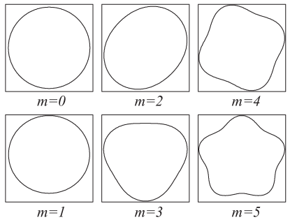
Figure 1: Phase space contour of longitudinal oscillation modes

Assuming that the phase space is scaled in such a way that a matched bunch in the linear region of the bucket is a circle, the $m$-th mode may be described by the formula

$$r=1+\epsilon_{B}\;sin(m\;\varphi).$$ (1)

Here, $(r,\varphi)$ are the polar coordinates of the bunch contour. It is obvious that an unperturbed bunch is obtained for $m=0$.

Fig. 1 shows the bunch contours for $\epsilon_{B}=0.1$.

II.2 Simplified Linear Differential Equations

We assume that the RF voltage is modulated according to

$$u(t)=\hat{u}_{0}(t)(1+\epsilon(t))\;sin(\varphi(t)-\Delta\varphi_{gap}(t))$$ (2)

where

$$\varphi(t)=\int\omega_{RF}(t)\;dt.$$

By definition, the reference particle arrives at the accelerating gap when $\varphi(t)=\varphi_{R}(t)+2\pi k$ is valid (the integer $k$ denotes the bunch repetition number); for a non-synchronous particle, the arrival time is defined by $\varphi(t)=\varphi_{R}(t)+2\pi k+\Delta\varphi(t)$. The magnetic field $B$ in the bending dipoles and the quantities $\hat{u}_{0}$, $\omega_{RF}$ and $\varphi_{R}$ are chosen in such a way that the reference particle follows the reference path. All these quantities vary slowly with time in comparison with the synchrotron oscillation. The modulation functions $\epsilon(t)$ and $\Delta\varphi_{gap}(t)$, however, may vary faster.

Thus, the nonlinear differential equations are

$$\Delta\dot{\varphi} = \frac{2\pi h\eta_{R}}{T_{R}\beta_{R}^{2}W_{R}}\Delta W$$ (3)

$$\Delta\dot{W} = \frac{Q\hat{u}_{0}}{T_{R}}[(1+\epsilon)\cdot sin(\varphi_{R}+\Delta\varphi-\Delta\varphi_{gap})-$$ (4)

$$- sin\;\varphi_{R}].$$

Here, $h$ denotes the harmonic number, $T_{R}$ the revolution time, $W_{R}=m_{0}c_{0}^{2}\gamma_{R}$ the total energy, and $\beta_{R}$, $\gamma_{R}$ are the relativistic Lorentz factors of the reference particle. With the transition gamma $\gamma_{T}$, $\eta_{R}=1/\gamma_{T}^{2}-1/\gamma_{R}^{2}$ is the phase slip factor. $Q$ is the charge of one single particle. $\Delta W$ and $\Delta\varphi$ are the energy and phase deviations of a non-synchronous particle with respect to the synchronous reference particle (cf. (Lee, 1999)).

For small values of $|\Delta\varphi-\Delta\varphi_{gap}|\ll 1$ we have

$$\Delta\dot{W}\approx\frac{Q\hat{u}_{0}cos\ \varphi_{R}}{T_{R}}(1+\epsilon)\left(\Delta\varphi-\Delta\varphi_{gap}+\frac{\epsilon\;tan\;\varphi_{R}}{1+\epsilon}\right).$$

Defining

$$\Delta\tilde{\varphi}_{gap}=\Delta\varphi_{gap}-\frac{\epsilon}{1+\epsilon}tan\;\varphi_{R}$$ (5)

leads to

$$\Delta\dot{W}\approx\frac{Q\hat{u}_{0}cos\;\varphi_{R}}{T_{R}}(1+\epsilon)(\Delta\varphi-\Delta\tilde{\varphi}_{gap}).$$ (6)

By a combination of equations (3) and (6), we get

$$\Delta{\ddot{\varphi}}=\frac{2\pi h\eta_{R}Q\hat{u}_{0}cos\;\varphi_{R}}{T_{R}^{2}\beta_{R}^{2}W_{R}}(1+\epsilon)(\Delta\varphi-\Delta\tilde{\varphi}_{gap}).$$

The synchrotron frequency is defined by

$$\omega_{S}=2\pi f_{S}=\sqrt{\frac{2\pi hQ\hat{u}_{0}(-\eta_{R}\;cos\;\varphi_{R})}{T_{R}^{2}\beta_{R}^{2}W_{R}}}$$

which yields

$$\Delta{\ddot{\varphi}}+\omega_{S}^{2}(1+\epsilon)\Delta\varphi=\omega_{S}^{2}(1+\epsilon)\Delta\tilde{\varphi}_{gap}.$$ (7)

By using the new variables

$$x=\Delta\varphi\mbox{\qquad}y=C\Delta{\dot{\varphi}}$$

we find:

$$\dot{x} = \frac{1}{C}y$$

$$\dot{y} = -C\omega_{S}^{2}(1+\epsilon)(x-\Delta\tilde{\varphi}_{gap})$$

For vanishing excitations with $\epsilon=0$ and $\Delta\tilde{\varphi}_{gap}=0$, we now require the trajectories to be circles:

$$x=cos(\omega_{S}t)\Rightarrow y=C\dot{x}=-C\omega_{S}sin(\omega_{S}t)\Rightarrow C=-\frac{1}{\omega_{S}}$$

Thus, we obtain (note that $C$ and $\omega_{S}$ vary slowly — therefore we neglect the time derivative):

$$\dot{x} = -\omega_{S}y$$ (8)

$$\dot{y} = \omega_{S}(1+\epsilon)(x-\Delta\tilde{\varphi}_{gap})$$ (9)

II.3 Behavior of Particle Bunches

Whereas equations (8) and (9) are valid for individual particles, we now consider bunches with $N$ particles.

II.3.1 Phase Oscillations

For the mean values, we find:

$$\bar{x}=\frac{1}{N}\sum_{k=1}^{N}x_{k}\mbox{\qquad}\bar{y}=\frac{1}{N}\sum_{k=1}^{N}y_{k}$$

$$\dot{\bar{x}}=\frac{1}{N}\sum_{k=1}^{N}\dot{x}_{k}=-\omega_{S}\frac{1}{N}\sum_{k=1}^{N}y_{k}=-\omega_{S}\bar{y}$$ (10)

$$\dot{\bar{y}}=\frac{1}{N}\sum_{k=1}^{N}\dot{y}_{k}=\omega_{S}(1+\epsilon)\frac{1}{N}\sum_{k=1}^{N}(x_{k}-\Delta\tilde{\varphi}_{gap})$$

$$\Rightarrow\dot{\bar{y}}=\omega_{S}(1+\epsilon)(\bar{x}-\Delta\tilde{\varphi}_{gap})$$ (11)

$$\ddot{\bar{x}}=-\omega_{S}\dot{\bar{y}}=-\omega_{S}^{2}(1+\epsilon)(\bar{x}-\Delta\tilde{\varphi}_{gap})$$ (12)

This equation for the bunch center has the same form as equation (7) for the individual particles.

II.3.2 Amplitude Oscillations

We define the following quantities:

$$a_{x}=\frac{1}{N}\sum_{k=1}^{N}x_{k}^{2}\mbox{\qquad}a_{y}=\frac{1}{N}\sum_{k=1}^{N}y_{k}^{2}\mbox{\qquad}\xi=\frac{1}{N}\sum_{k=1}^{N}x_{k}y_{k}$$

$$v_{x}=\frac{1}{N}\sum_{k=1}^{N}(x_{k}-\bar{x})^{2}=\frac{1}{N}\sum_{k=1}^{N}(x_{k}^{2}-2x_{k}\bar{x}+\bar{x}^{2})=a_{x}-\bar{x}^{2}$$

$$v_{y}=a_{y}-\bar{y}^{2}$$

Please note that $v_{x}$ corresponds to the variance of the quantities $x_{k}$ if a division by $N-1$ is used instead of the division by $N$. Since we are only interested in large numbers $N$, this difference is negligible.

The quantity $\sqrt{v_{x}}$ represents the bunch length whereas $\sqrt{v_{y}}$ represents the height of the bunch (this will later be analyzed in detail). We get:

$$\dot{a}_{x}=\frac{1}{N}\sum_{k=1}^{N}2x_{k}\dot{x}_{k}=-2\omega_{S}\xi$$

$$\dot{a}_{y}=\frac{1}{N}\sum_{k=1}^{N}2y_{k}\dot{y}_{k}=2\omega_{S}(1+\epsilon)\frac{1}{N}\sum_{k=1}^{N}y_{k}(x_{k}-\Delta\tilde{\varphi}_{gap})$$

$$\Rightarrow\dot{a}_{y}=2\omega_{S}(1+\epsilon)(\xi-\bar{y}\Delta\tilde{\varphi}_{gap})$$

$$\dot{\xi} = \frac{1}{N}\sum_{k=1}^{N}(\dot{x}_{k}y_{k}+x_{k}\dot{y}_{k})=$$

$$= -\omega_{S}a_{y}+\omega_{S}(1+\epsilon)(a_{x}-\bar{x}\Delta\tilde{\varphi}_{gap})$$

$$\dot{v}_{x}=\dot{a}_{x}-2\bar{x}\dot{\bar{x}}=-2\omega_{S}\xi+2\omega_{S}\bar{x}\bar{y}=-2\omega_{S}\alpha$$ (13)

Here we defined $\alpha=\xi-\bar{x}\bar{y}$ in order to have the same form in the expressions for $a_{x}$ and for $v_{x}$. We find:

$$\dot{v}_{y}=\dot{a}_{y}-2\bar{y}\dot{\bar{y}} = 2\omega_{S}(1+\epsilon)(\xi-\bar{y}\Delta\tilde{\varphi}_{gap})-$$

$$- 2\omega_{S}(1+\epsilon)\bar{y}(\bar{x}-\Delta\tilde{\varphi}_{gap})$$

$$\Rightarrow\dot{v}_{y}=2\omega_{S}(1+\epsilon)\alpha$$ (14)

$$\dot{\alpha} = \dot{\xi}-\dot{\bar{x}}\bar{y}-\bar{x}\dot{\bar{y}}=$$

$$= -\omega_{S}a_{y}+\omega_{S}(1+\epsilon)(a_{x}-\bar{x}\Delta\tilde{\varphi}_{gap})+$$

$$+ \omega_{S}\bar{y}^{2}-\omega_{S}(1+\epsilon)\bar{x}(\bar{x}-\Delta\tilde{\varphi}_{gap})$$

$$\Rightarrow\dot{\alpha}=-\omega_{S}v_{y}+\omega_{S}(1+\epsilon)v_{x}$$ (15)

Now we are able to derive a differential equation for $v_{x}$, i.e. for the bunch length oscillation.

Combining equations (13) and (14) yields:

$$\dot{v}_{y}=-(1+\epsilon)\dot{v}_{x}$$ (16)

We now combine equation (13) with equation (15):

$$\ddot{v}_{x}=2\omega_{S}^{2}v_{y}-2\omega_{S}^{2}(1+\epsilon)v_{x}$$ (17)

$$\Rightarrow\stackrel{{\scriptstyle...}}{{v}}_{x}=2\omega_{S}^{2}\dot{v}_{y}-2\omega_{S}^{2}(1+\epsilon)\dot{v}_{x}-2\omega_{S}^{2}\dot{\epsilon}v_{x}$$

Using equation (16), we finally get:

$$\stackrel{{\scriptstyle...}}{{v}}_{x}=-4\omega_{S}^{2}(1+\epsilon)\dot{v}_{x}-2\omega_{S}^{2}\dot{\epsilon}v_{x}$$ (18)

Please note that for $\epsilon=0$, the standard differential equation

$$\ddot{v}_{x}+(2\omega_{S})^{2}v_{x}=const.$$ (19)

is obtained which corresponds to an oscillation with the frequency $2\omega_{S}$. Due to the linearization, an initial quadrupole oscillation will continue forever.

Now we derive the differential equation for $v_{y}$, i.e. for the amplitude oscillation. Equation (14) yields:

$$\frac{\dot{v}_{y}}{1+\epsilon}=2\omega_{S}\alpha$$

The time derivative is

$$\frac{\ddot{v}_{y}(1+\epsilon)-\dot{\epsilon}\dot{v}_{y}}{(1+\epsilon)^{2}}=-2\omega_{S}^{2}v_{y}+2\omega_{S}^{2}(1+\epsilon)v_{x}$$

where we used eqn. (15) on the right side. We divide by $(1+\epsilon)$:

$$\frac{\ddot{v}_{y}}{(1+\epsilon)^{2}}-\frac{\dot{\epsilon}\dot{v}_{y}}{(1+\epsilon)^{3}}=-2\omega_{S}^{2}\frac{v_{y}}{1+\epsilon}+2\omega_{S}^{2}v_{x}$$

Now another time derivative leads to $\dot{v}_{x}$ on the right side such that we can use eqn. (16) to eliminate $v_{x}$ completely. After some steps, one obtains:

$$\stackrel{{\scriptstyle...}}{{v}}_{y}-\frac{3\ddot{v}_{y}\dot{\epsilon}}{1+\epsilon}+\dot{v}_{y}\left(4\omega_{S}^{2}(1+\epsilon)-\frac{\ddot{\epsilon}}{1+\epsilon}+\frac{3\dot{\epsilon}^{2}}{(1+\epsilon)^{2}}\right)=$$

$$=2\omega_{S}^{2}\dot{\epsilon}v_{y}$$ (20)

This differential equation for $v_{y}$ differs from eqn. (18) for $v_{x}$ only by terms that are of higher-order with respect to $\epsilon$. Furthermore, the sign of the excitation term $2\omega_{S}^{2}\dot{\epsilon}v_{y}$ is different for $v_{x}$ and $v_{y}$ which matches the expectations since the bunch is short when its amplitude is high whereas the bunch is long when its amplitude is small.

Please note that we have not introduced any approximations to derive the differential equations (18) and (20) from equations (8) and (9).

According to (Kamke, 1956), these differential equations have the following solution:

$$v_{x}=C_{x1}w_{x1}^{2}+C_{x2}w_{x1}w_{x2}+C_{x3}w_{x2}^{2}$$ (21)

$$v_{y}=C_{y1}w_{y1}^{2}+C_{y2}w_{y1}w_{y2}+C_{y3}w_{y2}^{2}$$ (22)

The functions $w_{x1}$ and $w_{x2}$ are the linearly independent solutions of

$$\ddot{w}_{x}+\omega_{S}^{2}(1+\epsilon)w_{x}=0,$$

whereas the functions $w_{y1}$ and $w_{y2}$ are the linearly independent solutions of

$$\ddot{w}_{y}-\frac{\dot{\epsilon}}{1+\epsilon}\dot{w}_{y}+\omega_{S}^{2}(1+\epsilon)w_{y}=0.$$

In the trivial case $\epsilon=0$, we may choose

$$w_{x1}=w_{y1}=cos(\omega_{S}t)\mbox{,\qquad}w_{x2}=w_{y2}=sin(\omega_{S}t)$$

as a solution. Due to equations (21) and (22), $v_{x}$ and $v_{y}$ will oscillate with twice the frequency which is in compliance with eqn. (19).

In appendix A, it is shown that the following differential equations are valid as an approximation for small deviations from the matched bunch shape:

$$\ddot{\bar{x}}+\omega_{S}^{2}\bar{x}=\omega_{S}^{2}\Delta\tilde{\varphi}_{gap}$$ (23)

$$\ddot{v}_{x}+4\omega_{S}^{2}(v_{x}-v_{0})=-2\omega_{S}^{2}v_{0}\epsilon.$$ (24)

II.4 Revolution Time in Phase Space

The revolution frequency of off-center particles in the nonlinear bucket in phase space is given by

$$f_{S,nonlinear}(\Delta\varphi)=f_{S}\frac{\pi}{2K\left(\sin\frac{\Delta\varphi}{2}\right)}$$ (25)

(cf. (Lee, 1999)). Here, $\Delta\varphi$ is the maximum phase deviation of the particle and $K$ is the complete elliptic integral of the first kind. Due to the longitudinal emittance of the bunch in the nonlinear bucket, the quantities $\bar{x}$ and $v_{x}$ will not oscillate with the frequency $f_{S}$ and $2f_{S}$, respectively, but with reduced frequencies $f_{S,eff}$ and $2f_{S,eff}$.

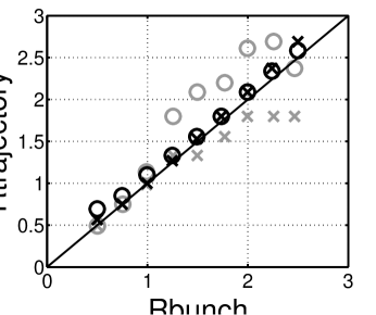
Figure 2: Effective phase deviation $\Delta\varphi_{eff}$ for different bunch sizes and different modes of oscillation ( $\times$: dipole mode, $\circ$: quadrupole mode, black: homogeneous distribution, grey: Gaussian distribution)

We now analyzed how $f_{S,eff}$ depends on the size of the bunch. For this purpose, the solutions of the linearized ODEs (23) and (24) were compared with a nonlinear tracking simulation for an initial bunch with an example shape given by

$$r=r_{0}\left[1+0.1\cos(\varphi)+0.2\cos(2\varphi)\right].$$

The longitudinal emittance is determined by the parameter $r_{0}$. Due to the mismatch of the bunch, $v_{x}$ and $v_{y}$ perform oscillations around the average values $v_{x0}$ and $v_{y0}$, respectively. Please note that one has $v_{x0}<v_{y0}$ since the nonlinear bucket has the shape of an eye instead of a circle. For each run of the simulation, the average value $v_{x0}$ was determined as a measure for the bunch length. Each run of the nonlinear tracking simulation also leads to a certain oscillation frequency, and we determined $\Delta\varphi$ such that this frequency matches $f_{S,nonlinear}(\Delta\varphi)$ for $\bar{x}$ or $2f_{S,nonlinear}(\Delta\varphi)$ for $v_{x}$, respectively. As a result, the effective phase deviation $\Delta\varphi=:\Delta\varphi_{eff}$ and $v_{x0}$ are determined for each simulation run.

Fig. 2 shows the relation between these two quantities. It is obvious that the effective synchrotron frequency $f_{S,eff}$ is approximately determined by

$$f_{S,eff}=f_{S,nonlinear}(\Delta\varphi_{eff})$$ (26)

if

$$\Delta\varphi_{eff}=2\sqrt{v_{x0}}$$ (27)

is used.

II.5 Interpretation of $\bar{x}$ and $v_{x}$

According to the equations

$$\bar{x}\approx-\varphi_{1},\mbox{\qquad}v_{x}\approx 2\;ln\frac{2\bar{i}}{A_{1}}=2\;ln\frac{A_{0}}{A_{1}}$$ (28)

the mean value $\bar{x}$ and the variance $v_{x}$ may approximately be converted into the phase $\varphi_{1}$ and the amplitude $A_{1}$ of the fundamental harmonic component. $A_{0}$ is the zeroth Fourier component, and $\bar{i}$ is the DC component of the beam signal. The approximation (28) was derived for an elliptical Gaussian bunch with a large number of particles. It also holds for a homogeneous distribution.

We will show now that equation (28) is also a good approximation for larger bunches and even if a significant amount of filamentation is present.

Table 1: Simulation parameters

Synchrotron circumference $l_{R}$	$216.72\;\rm m$
Transition gamma $\gamma_{T}$	$5.45$
Ion species	$\rm{}^{40}Ar^{18+}$
Kinetic energy	$11.4\;\rm MeV/u$
RF amplitude $\hat{u}_{0}$	$10\;\rm kV$
Harmonic number $h$	8
Synchrotron frequency $f_{S}$	$3312\;\rm Hz$
Revolution time $T_{R}$	$4.66\;\rm\mu s$
Parameters resulting from the initial conditions:
$v_{x0}$	$0.773$
$\Delta\varphi_{eff}=2\sqrt{v_{x0}}$	$1.7584$
$f_{S,eff}/f_{S}$	$0.8087$

For the parameters shown in Table 1, solutions for the following models were generated numerically:

1. A nonlinear particle tracking simulation. The parameters $\bar{x}$ and $v_{x}$ are calculated.

2. An FFT analysis of the previous result was made which leads to the phase $\varphi_{1}$, the amplitude $A_{1}$ and the DC component $A_{0}/2=\bar{i}$. Based on these parameters, an approximation for $\bar{x}$ and $v_{x}$ is calculated using eqn. (28).

3. Solution of the nonlinear ordinary differential equations (ODE) (12) and (18).

4. Solution of the linearized ODE (23) and (24).

For the last two models 3 and 4, the effective synchrotron frequency $f_{S,eff}$ was used instead of $f_{S}$.

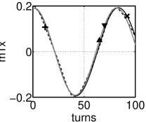
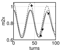
Figure 3: Mean value $\bar{x}$ and variance $v_{x}$ versus time for $\omega_{S,eff}=0.8\;\omega_{S}$. The initial bunch is a homogeneous distribution according to $r=1.6\left[1+0.1\cos(\varphi)+0.2\cos(2\varphi)\right]$. No excitation is applied ( $\times$: nonlinear tracking simulation, $+$: result of the FFT using eqn. (28), $\triangle$: nonlinear ODE, $\nabla$: linearized ODE).

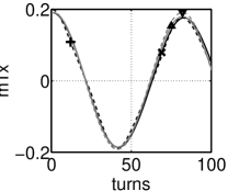
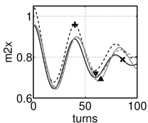
Figure 4: Mean value $\bar{x}$ and variance $v_{x}$ versus time for $\omega_{S,eff}=0.8\;\omega_{S}$. The initial bunch is a homogeneous distribution according to $r=1.6\left[1+0.1\cos(\varphi)+0.2\cos(2\varphi)\right]$. An excitation $\epsilon=0.04\;\sin(2\omega_{S,eff}t+\pi)$ is applied ( $\times$: nonlinear tracking simulation, $+$: result of the FFT using eqn. (28), $\triangle$: nonlinear ODE, $\nabla$: linearized ODE).

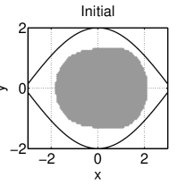
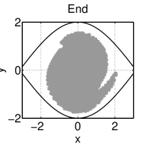
Figure 5: Phase space distribution at the beginning (left diagram) and at the end (right diagram) of the simulation. The initial bunch is a homogeneous distribution according to $r=1.6\left[1+0.1\cos(\varphi)+0.2\cos(2\varphi)\right]$ (mismatch of both, bunch center and bunch length). No excitation is applied (same case as in Fig. 3).

Fig. 3 shows the result for a mismatched bunch without additional excitation, and Fig. 5 shows the corresponding phase space plots. Fig. 4 shows the result for the same mismatched bunch with an additional excitation. These examples show the following:

• The formula (28) describes the oscillation very accurately, but there is a small DC offset which may be relevant for small oscillation amplitudes. As we will see later, the DC component is usually not of interest for the control loop design.

• The models 1 (marker $\times$ in the diagrams) and 2 (marker $+$ in the diagrams) match very well even for comparatively large bunches and for mismatches including filamentation. This clearly shows that the quantities $\bar{x}$ and $v_{x}$ may be used instead of $\varphi_{1}$ and $A_{1}$ if the approximation (28) is used.

• The models 1 and 2 include Landau damping since they are based on nonlinear tracking equations. The models 3 (marker $\triangle$) and 4 (marker $\nabla$) cannot show Landau damping since they are based on linear tracking equations.

• During the first oscillation period, all models match very well which indicates that all models may be used for designing feedback systems.

• Fig. 4 shows that the excitation with $2f_{S,eff}$ initially leads to a damping of the amplitude oscillation. The initial damping rates of all four models are similar. This is a further confirmation that the models may be used for control loop design.

II.6 Phase and Amplitude Oscillations of the Normal Modes

We now consider the normal modes introduced in section II.1. If one assumes a homogenous particle distribution inside the bunch contour defined by equation (1), one may calculate the phase and amplitude oscillations analytically. The integrals that have to be solved are the following ones:

$$M_{0}=\int_{0}^{2\pi}\int_{0}^{r_{max}}r\;dr\;d\varphi$$

$$\bar{x}=\frac{1}{M_{0}}\int_{0}^{2\pi}\int_{0}^{r_{max}}x\;r\;dr\;d\varphi$$

$$\bar{y}=\frac{1}{M_{0}}\int_{0}^{2\pi}\int_{0}^{r_{max}}y\;r\;dr\;d\varphi$$

$$a_{y}=\frac{1}{M_{0}}\int_{0}^{2\pi}\int_{0}^{r_{max}}y^{2}\;r\;dr\;d\varphi\mbox{,\qquad}v_{y}=a_{y}-\bar{y}^{2}$$

Here, the following equations were used:

$$r_{max}=1+\epsilon_{B}\;sin\left[m\;(\varphi-\varphi_{0})\right]$$

$$x=r\;cos\;\varphi\mbox{\qquad}y=r\;sin\;\varphi$$

The following results are obtained:

$$M_{0}=\left\{\begin{array}[]{ll}\pi&\mbox{for }m=0\\ \pi\left(1+\frac{1}{2}\epsilon_{B}^{2}\right)&\mbox{for }m>0\end{array}\right.$$

$$\bar{x}=\left\{\begin{array}[]{ll}-\frac{\left(\epsilon_{B}+\frac{1}{4}\epsilon_{B}^{3}\right)sin\;\varphi_{0}}{1+\frac{1}{2}\epsilon_{B}^{2}}&\mbox{for }m=1\\ 0&\mbox{for }m\neq 1\end{array}\right.$$

$$\bar{y}=\left\{\begin{array}[]{ll}\frac{\left(\epsilon_{B}+\frac{1}{4}\epsilon_{B}^{3}\right)cos\;\varphi_{0}}{1+\frac{1}{2}\epsilon_{B}^{2}}&\mbox{for }m=1\\ 0&\mbox{for }m\neq 1\end{array}\right.$$

$$v_{y}=\left\{\begin{array}[]{ll}\frac{1}{4}&\mbox{for }m=0\\ \frac{1}{4}\frac{1+\frac{3}{2}\epsilon_{B}^{2}+\frac{7}{8}\epsilon_{B}^{4}+\frac{1}{16}\epsilon_{B}^{6}-\frac{1}{2}\epsilon_{B}^{2}\;cos(2\varphi_{0})}{\left(1+\frac{1}{2}\epsilon_{B}^{2}\right)^{2}}&\mbox{for }m=1\\ \frac{1}{4}\frac{1+3\epsilon_{B}^{2}+\frac{3}{8}\epsilon_{B}^{4}+\left(2\epsilon_{B}+\frac{3}{2}\epsilon_{B}^{3}\right)sin(2\varphi_{0})}{1+\frac{1}{2}\epsilon_{B}^{2}}&\mbox{for }m=2\\ \frac{1}{4}\frac{1+3\epsilon_{B}^{2}+\frac{3}{8}\epsilon_{B}^{4}}{1+\frac{1}{2}\epsilon_{B}^{2}}&\mbox{for }m>2\\ \end{array}\right.$$

We see that only the mode $m=1$ shows a phase modulation with the frequency $f_{S}$ (since $\bar{x}$ is periodic with respect to $\varphi_{0}$). The mode $m=1$ also shows an amplitude modulation with the frequency $2f_{S}$ (since $v_{y}$ is periodic with respect to $2\varphi_{0}$), but this is a parasitic effect caused by the fact that the bunch shape is only approximately circular. The slight deformation causes the modulation of the order $\epsilon_{B}^{2}$. Apart from this exception, only the mode $m=2$ shows an amplitude modulation with the frequency $2f_{S}$ of the order $\epsilon_{B}$. The modes $m>2$ neither show a phase modulation nor an amplitude modulation.

II.7 Spectrum of Dipole Oscillation

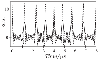
Figure 6: Visualization of the partial sums of the series in eqn. (29) for $T_{R}=1\;\mu s$, $T_{S}=8\;\mu s$, $\Delta t=0.3\;\mu s$ (solid line: summation up to $n=20$, dashed line: summation up to $n=50$)

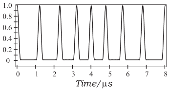
Figure 7: Dipole oscillation of $cos^{2}$-shaped bunches for $T_{R}=1\;\mu s$, $T_{S}=8\;\mu s$, $\Delta t=0.3\;\mu s$, $\Omega=18/T_{R}$ (summation up to $n=100$)

In appendix B, we prove the formula

$$\sum_{k=-\infty}^{+\infty}\delta\left(t-kT_{R}-\Delta t\;sin\left(2\pi k\frac{T_{R}}{T_{S}}\right)\right)=$$

$$=\frac{1}{T_{R}}+\sum_{n=1}^{\infty}A_{n}cos(n\omega_{S}t)$$ (29)

for $\Delta t<T_{R}/2$ where

$$A_{n}=\frac{2}{T_{S}}\left[1+\sum_{k=1}^{\frac{T_{S}}{T_{R}}-1}cos\left(n\omega_{S}\left[kT_{R}+\Delta t\,sin\frac{2\pi kT_{R}}{T_{S}}\right]\right)\right]$$

and $T_{S}/T_{R}$ is a positive integer.

Fig. 6 shows the graph of two different partial sums of the series on the right side of eqn. (29) for one period $T_{S}=2\pi/\omega_{S}$. It is obvious that the peaks become the higher the more terms are added. One also sees that the pulse density is high in the middle whereas it is low at the beginning and at the end of the period. This is the expected behavior for the dipole oscillation under consideration.

A real beam signal consists of pulses with finite height and length instead of the Dirac pulses. Let us assume that such a single finite pulse centered at $t=0$ is given by the function $x(t)$. If we write the above-mentioned train of Dirac pulses as

$$h(t)=\sum_{k=-\infty}^{+\infty}\delta(t-T_{k}),$$

we get the convolution

$$y(t)=h(t)*x(t)=\sum_{k=-\infty}^{+\infty}x(t-T_{k}),$$ (30)

which corresponds to the desired beam signal. This signal still shows dipole oscillations if $T_{k}$ is implicitly defined by eqn. (29). Since

$$h(t)=\sum_{n=-\infty}^{+\infty}c^{(h)}_{n}e^{jn\omega_{S}t}$$

is given by a Fourier series, the corresponding Fourier transform is

$$H(j\omega)=2\pi\sum_{n=-\infty}^{+\infty}c^{(h)}_{n}\delta(\omega-n\omega_{S})$$

where $c^{(h)}_{n}=\frac{A_{n}}{2}$. The Fourier transform of eqn. (30) is

$$Y(j\omega) = H(j\omega)X(j\omega)=$$

$$= 2\pi\sum_{n=-\infty}^{+\infty}c^{(h)}_{n}X(jn\omega_{S})\delta(\omega-n\omega_{S}).$$

This is again a Fourier series whose Fourier coefficients are given by

$$c^{(y)}_{n}=c^{(h)}_{n}X(jn\omega_{S}).$$

For beam pulses that have the form

$$x(t)=\left\{\begin{array}[]{ll}cos^{2}\left(\frac{\Omega}{2}t\right)&\mbox{\quad for }-\pi\leq\Omega t\leq\pi\\ 0&\mbox{\quad elsewhere}\end{array}\right.$$

one may — as a simple but still realistic example — derive the Fourier transform

$$X(j\omega)=\left\{\begin{array}[]{ll}\frac{\pi}{\Omega}\frac{si\left(\pi\frac{\omega}{\Omega}\right)}{1-\left(\frac{\omega}{\Omega}\right)^{2}}&\mbox{ for }|\omega|\neq\Omega\\ \frac{\pi}{2\Omega}&\mbox{ for }|\omega|=\Omega\end{array}\right.$$

An example for such a bunch train with dipole oscillations is shown in Fig. 7. In this example, we have chosen an unrealistic synchrotron period of $T_{S}=8\;\mu s$ in order to be able to show the result in a diagram. For a realistic synchrotron period of $T_{S}=1000\;\mu s$, the Fourier coefficients are shown in Table 2. Please note that the following condition has to be fulfilled since the bunch has to fit into the bucket even if the maximum bunch offset $\Delta t$ occurs:

$$\frac{\pi}{\Omega}+\Delta t<\frac{T_{R}}{2}$$

Table 2: Fourier coefficients $a^{(y)}_{n}=2c^{(y)}_{n}$ of a bunch train with dipole ocscillations ($T_{R}=1\;\mu s$, $T_{S}=1000\;\mu s$, $\Delta t=0.3\;\mu s$, $\Omega=18/T_{R}$)

	$f_{R}$	$2f_{R}$	$3f_{R}$	$4f_{R}$
$-5f_{S}$	0.0016819	0.0267036	0.0545552	0.0222028
$-4f_{S}$	0.0087296	0.0618662	0.0634047	0.0012028
$-3f_{S}$	0.0355937	0.1048087	0.0351619	-0.0208789
$-2f_{S}$	0.1050056	0.1050122	-0.0260749	-0.0177420
$-1f_{S}$	0.1875566	0.0065220	-0.0534534	0.0114866
$+0f_{S}$	0.0937025	-0.1014007	0.0073288	0.0207027
$+1f_{S}$	-0.187475	-0.0061292	0.0533306	-0.0115380
$+2f_{S}$	0.1055102	0.1045001	-0.0263491	-0.0175559
$+3f_{S}$	-0.0361045	-0.1048387	-0.0345397	0.0208711
$+4f_{S}$	0.0089756	0.0622868	0.0629741	0.0008722
$+5f_{S}$	-0.0017600	-0.0271106	-0.0545328	-0.0217486

The following points are observed:

• The dominant spectral lines do not occur at $pf_{R}\pm f_{S}$ in general. In our example, this is only valid for $p=1$.

• Although an ideal dipole mode was modeled, spectral lines also exist at $pf_{R}\pm 2f_{S}$, $pf_{R}\pm 3f_{S}$, etc. This is normally interpreted as a quadrupole, sextupole, etc. component in the oscillation.

• The sidebands are not symmetric with respect to the harmonics of the revolution frequency.

When $\Delta t$ is reduced significantly in this example (i.e. for smaller dipole oscillations), the dominant spectral lines are located at $pf_{R}\pm f_{S}$ as expected, and the symmetry is also improved. The pure existence of Fourier components at $pf_{R}\pm 2f_{S}$, $pf_{R}\pm 3f_{S}$, etc. remains, however (their magnitude is smaller than that at $pf_{R}\pm f_{S}$).

It has to be emphasized that the validity of these observations is very general. Even though the example was a special one, the formulas for the Fourier series are not based on any approximations.

III Sextupole Mode Generation

In this section, we try to excite a sextupole oscillation by a phase modulation with

$$\Delta\varphi_{gap}=\frac{\pi}{18}\;sin(3\omega_{S}t)$$

which corresponds to a phase deviation of $\pm 10^{\circ}$. The parameters defined in Table 1 are used, and a matched bunch ($r=1$) is assumed at the beginning.

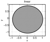
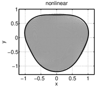
Figure 8: Phase space at $t=1.12T_{S}$ for an excitation with $3f_{S}$ (Left diagram: linear tracking equations, right diagram: nonlinear tracking equations)

After a time $t=1.12\;T_{S}$, the phase space distribution shown in Fig. 8 is obtained. The left diagram shows that no typical sextupole distribution is obtained if linearized tracking equations are used. In the right diagram one can see that the original nonlinear tracking equations lead to a sextupole distribution whose contour is compliant with equation (1) for $m=3$. Matching the contour to the particle cloud leads to

$$r=1+0.1\;sin(\varphi-\pi)+0.1\;sin(3\varphi).$$

This shows that both, a dipole and a sextupole mode is excited. It has to be emphasized that an excitation of the sextupole mode is only possible in the nonlinear bucket. This was also verified using the program package ESME (MacLachlan, 1997) and can furthermore be shown analytically (Gross, 2009).

IV Application of Models

Using the models described in section II, an example for a specific longitudinal damping system is presented in the following. The theoretical results are compared with measurement data.

IV.1 Beam Phase Control and Quadrupole Damping System

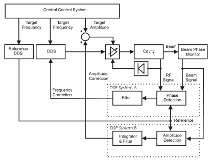
Figure 9: Block diagram of the beam phase control system and the quadrupole damping system

The models presented before were used to analyze an RF system that is displayed in Fig. 9. A DDS module provides an RF master signal with the frequency provided by the central control system. An amplitude control loop which is not considered in the paper at hand makes sure that the detected amplitude of the cavity RF signal matches the target amplitude provided by the central control system.

A phase detection algorithm in DSP system A compares the phase of the cavity voltage with the phase of the beam signal. This phase difference is then processed by a digital bandpass filter with $f_{S}$ belonging to the passband. After applying a proportional gain, the filter output is used to modify the DDS frequency. For analyzing the loop characteristics, the DDS may be regarded as an integrator with respect to the phase. The loop A ensures that coherent dipole oscillations with a frequency approximately equal to $f_{S}$ will be damped.

In DSP system B, an amplitude detection algorithm is applied to the beam signal. This signal is fed to a digital filter with a passband frequency of about $2f_{S}$. In contrast to the dipole oscillation damping loop A mentioned before, there is no intrinsic integrator in loop B. Therefore, an additional integrator is implemented in DSP system B. The resulting signal is used to modify the target amplitude in order to damp quadrupole oscillations.

Both DSP systems need a reference signal which allows them to detect RF signals at the relevant frequency. For this purpose a reference DDS is used.

IV.2 Analytic Model for the Damping System

The first natural step to analyze a control loop system like that shown in Fig. 9 is to linearize the building blocks in order to get transfer functions in the Laplace domain. For example, eqn. (23) directly leads to the well-known (Boussard, 1991) beam transfer function

$$G_{1}(s)=\frac{\Delta\varphi_{B}}{\Delta\tilde{\varphi}_{gap}}=\frac{\omega_{S}^{2}}{s^{2}+\omega_{S}^{2}}$$

where $\Delta\varphi_{B}=\bar{x}$ is the beam phase. Eqn. (24) is more difficult to interpret. In a well-designed quadrupole damping system, no significant emittance blow-up will occur. Therefore, the variance $v_{0}$ is a constant which is defined by the longitudinal emittance of the bunches. Hence, by defining

$$\Delta v_{x}=v_{x}-v_{0}$$

we may rewrite eqn. (24) in the form

$$\Delta\ddot{v}_{x}+4\omega_{S}^{2}\;\Delta v_{x}=-2\omega_{S}^{2}v_{0}\epsilon.$$

which corresponds to the transfer function

$$G_{2}(s)=\frac{\Delta v_{x}}{-2v_{0}\epsilon}=\frac{\omega_{S}^{2}}{s^{2}+4\omega_{S}^{2}}.$$

which is also known from literature (Boussard, 1991).

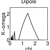
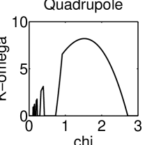
Figure 10: Stability diagram for damping dipole (left diagram) and quadrupole modes (right diagram), $T_{d}=10\;\rm\mu s$, $f_{S}=3312\;\rm Hz$

By using the transfer function $G_{1}(s)$, the beam-phase control loop was analyzed in (Klingbeil et al., 2007). In an analog way we took $G_{2}(s)$ to analyze the quadrupole damping loop. In both cases, the same type of filter specified in (Klingbeil et al., 2007) was used. Fig. 10 shows the region of stability for both, the dipole and the quadrupole damping system. Formulas for the first one can be found in (Klingbeil et al., 2007), the stability region for the latter one is given by

$$K_{crit}=\min_{p}K_{p,crit}$$

where

$$\frac{K_{p,crit}}{\omega_{S}}=16\frac{\xi|1-\xi^{2}|}{1-\cos\frac{\pi\xi}{\chi}},$$

$$\xi=\left\{\begin{array}[]{ll}\frac{p-\frac{1}{2}}{\frac{1}{\chi}+4T_{d}f_{S}}&\mbox{ for }\xi<1\mbox{ and }p\in\{1,3,5,\dots\}\\ \frac{p+\frac{1}{2}}{\frac{1}{\chi}+4T_{d}f_{S}}&\mbox{ for }\xi>1\mbox{ and }p\in\{1,3,5,\dots\}\end{array}\right.$$

and

$$\chi=\frac{f_{pass}}{2f_{S}}.$$

These results were derived in the same way as described in (Klingbeil et al., 2007). The stability diagram is in compliance with the measurement results.

IV.3 Measurement Results

Table 3: Beam experiment parameters

Synchrotron circumference $l_{R}$	$216.72\;\rm m$
Transition gamma $\gamma_{T}$	$5.45$
Ion species	$\rm{}^{40}Ar^{18+}$
Kinetic energy	$11.4\;\rm MeV/u$
DC beam current $\bar{i}$	$2\;\rm mA$
RF amplitude $\hat{u}_{0}$	step from $5$ to $10\;\rm kV$
Harmonic number $h$	8
Synchrotron frequency $f_{S}$ at $10\;\rm kV$	$3312\;\rm Hz$
Revolution time $T_{R}$	$4.66\;\rm\mu s$

Table 4: Control loop parameters for measurement and simulation

Delay time dipole damping system	$10\;\rm\mu s$
Delay time quadrupole damping system	$10\;\rm\mu s$
Filter frequency quadrupole damping system	$9000\;\rm Hz$
Filter frequency dipole damping system	$3500\;\rm Hz$
Sampling frequency of FIR filters	$375.44\;\rm kHz$

In order to verify the models presented here, a closed-loop analysis was performed, and the results were compared with the measurement results obtained in a beam experiment. Table 3 shows the beam experiment conditions. In this experiment, a matched beam in a stationary bucket generated by an RF voltage of $5\;\rm kV$ was present. By doubling the voltage instantaneously, quadrupole oscillations were excited intentionally. Excitations of this magnitude will never occur in practice — they were only used to show the functionality of the system and the validity of the theory.

The upper diagram in Fig. 11 shows the measured amplitude of the beam signal. The lowest trace is obtained if neither the beam phase control nor the quadrupole damping system are switched on. The oscillation frequency is lower than $2\;f_{S}$ (period of $200\;\mu s$ instead of $150\;\mu s$) since the nonlinearity of the bucket cannot be neglected for the momentum spread of the bunch. Due to Landau damping, the oscillation becomes weaker with time. The trace in the middle of Fig. 11 shows that the damping time is reduced significantly in comparison with Landau damping if the quadrupole damping system is switched on. For the last uppermost trace in Fig. 11 not only this quadrupole damping system was switched on, but also the beam phase control system which damps the coherent dipole mode. It is obvious that both control loops work together without negative influence.

The upper diagram in Fig. 12 shows the measured phase of the beam signal. A phase offset was introduced for each trace in order to have the same order as in Fig. 11. Therefore, the lowest trace again corresponds to both control loops being off which leads to Landau damping only. As expected, the oscillation period of $400\;\rm\mu s$ equals twice the period of the quadrupole oscillation. The uppermost trace shows that the coherent dipole oscillation is damped faster than the Landau damping time if both control loops are switched on. The trace in the middle indicates that switching on the quadrupole damping system while disabling the dipole damping system increases the excitation of the coherent dipole mode (in comparison with the case that both loops are disabled).

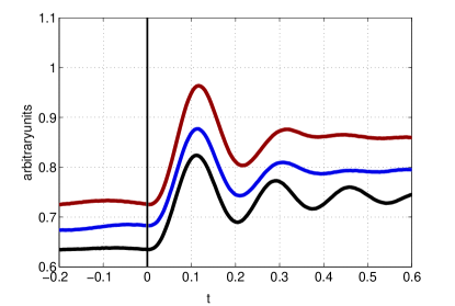
Figure 11: Measurement results (upper diagram) and simulation results (lower diagram) for beam signal amplitude (Uppermost trace: both control loops for quadrupole damping and for dipole damping on, trace in the middle: only control loop for quadrupole damping on, lowest trace: both control loops off)

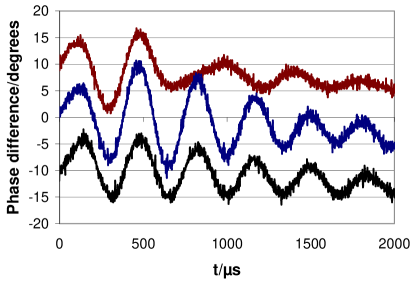
Figure 12: Measurement results (upper diagram) and simulation results (lower diagram) for beam signal phase (Uppermost trace: both control loops for quadrupole damping and for dipole damping on, trace in the middle: only control loop for quadrupole damping on, lowest trace: both control loops off)

Figure 13: Measured beam signal (Dotted line: before voltage jump, solid line: first maximum after voltage jump)

IV.4 Simulation

The experiments were compared with nonlinear tracking simulations. The simulation program used nonlinear discrete mapping equations in $\Delta\varphi$ and $\Delta W/\omega_{RF}$ for the longitudinal dynamics. The particle positions in phase space were then converted to the $(x,y)$ plane with the variables $x=\Delta\varphi$ and $y=-\Delta\dot{\varphi}/\omega_{S}$. The beam current signal was calculated as a histogram using bins on the $\Delta\varphi$-axis. The beam signal amplitude and phase were obtained by an FFT of the beam current signal.

Since coherent modes were excited in the experiment, only one bunch was simulated and compared with one bunch of the measured bunch signals at $h=8$. The macro-particles of the simulated bunch were initialized randomly with a Gaussian probability distribution. The matched bunch was injected at the gap voltage of $5~{}\rm kV$. The gap voltage was modeled according to eqn. (2) where $\Delta\varphi_{gap}$ is the output of the dipole feedback loop and $\epsilon$ of the quadrupole feedback loop, respectively. The dipole feedback loop comprised an FIR filter and the dynamics of the DDS module which was modeled as an integrator (see Fig. 9 for the control loop topology). The input of the dipole feedback was the beam signal phase. The quadrupole feedback loop consisted of an FIR filter and an additional integral controller. The input of the quadrupole feedback was the absolute beam signal amplitude $A_{1}(t)$. The control loop parameters are given in Table 4.

The cavity and its control loop dynamics were taken into account by a time constant of $T_{cav}=20~{}\rm\mu s$. In the experiment, the voltage step from $5~{}\rm kV$ to $10~{}\rm kV$ also causes a small phase shift due to the nonlinearity of the cavity system (detuning effect). Therefore, this phase shift was also added to the simulation.

IV.5 Simulation Results and Comparison with Measurement

In order to simulate the scenarios presented in section IV.3 using the procedure described in section IV.4, it was necessary to determine the beam parameters. For all three cases (only Landau damping without control loops, only quadrupole damping, quadrupole and dipole damping), the rms width of the beam signal before the voltage jump was determined by matching a Gaussian distribution to those measurement results which were valid before the voltage jump occurs. This fitting procedure leads to the parameters shown in Table 5. Since the bunch was matched before the voltage jump occurred, we have $v_{x}=v_{x0}$ and $v_{y}=v_{y0}$.

Table 5: Variances of measured beam before voltage step

	$v_{x}=v_{x0}$	$v_{y}=v_{y0}$	$v_{0}=\sqrt{v_{x}v_{y}}$
only Landau	1.135	0.691	0.886
damping
quadrupole	1.317	0.791	1.021
damping on
dipole and quadrupole	1.313	0.792	1.020
damping on

It is obvious that almost the same parameters are obtained for the three measurements which means that the beam quality was reproducible during the beam experiment.

The voltage step from $5~{}\rm kV$ to $10~{}\rm kV$ leads to an increase of the bucket area by a factor of $\sqrt{2}$. Therefore, the relative bunch area $v_{0}$ will be $1/\sqrt{2}$ times smaller than before the step. The $(x,y)$ phase space was defined in such a way that the trajectories are circles. Therefore, $v_{x0}$ and $v_{y0}$ will also be $1/\sqrt{2}$ times smaller than before the step. In the case that no control loops are present (only Landau damping), this leads to $v_{x0}=1.135/\sqrt{2}=0.803$. This value which is valid for the new larger bucket immediately after the voltage step was therefore approximately assumed in Table 1. Based on equations (26) and (27), it leads to $f_{S,eff}=0.8f_{S}=2650\;\rm Hz$ which is in agreement with the measurement.

Now that the initial conditions for the beam were fixed, further parameters shown in Table 4 had to be adopted from the beam experiment. The only two parameters that were now still open were the proportional gain factors for the two control loops. As Figures 11 and 12 show, the proper choice of these gain factors leads to a good agreement between measurement and simulation.

IV.6 Geometrical Interpretation for Matched Bunches

For the first case (only Landau damping) we found $v_{x0}=1.135$ before the voltage step occurs. According to equation (27) this leads to

$$x_{eff}=\Delta\varphi_{eff}=2.13.$$

The $(x,y)$ phase space leads to a bucket with the bucket length $2x_{max}$ where $x_{max}=\pi$ and with the bucket height $2y_{max}$ where $y_{max}=2$. The bucket area equals $16$. If $x$ is increased from $0$ to $\pi$, the ratio

$$\frac{y}{x}=\frac{\sqrt{2(1-\cos\;x)}}{x}$$

will decrease from $1$ (circular trajectory) to $2/\pi$ (separatrix). If we apply this formula for $x_{eff}$, we obtain $y_{eff}/x_{eff}=0.8214$. Due to equation (27) this leads to $v_{y0}/v_{x0}=0.67$. This is close to the ratio $v_{y0}/v_{x0}=0.61$ derived from the data in Table 5. This is an indication that $x_{eff}=2\sqrt{v_{x0}}$ and $y_{eff}=2\sqrt{v_{y0}}$ may actually be interpreted as the effective half axes of the bunch. In our case this leads to a bucket filling factor of

$$\frac{\pi x_{eff}y_{eff}}{16}=\frac{\pi}{16}x_{eff}^{2}\frac{y_{eff}}{x_{eff}}=73\;\%$$

This is close to the value $\pi v_{0}/4=70\;\%$ based on the values in Table 5.

Instead of the fitting procedure applied above, the value $x_{eff}=\Delta\varphi_{eff}$ may also be found by determining the two-sigma length of the bunch (in our case, the one-sigma length derived from the measured bunch profile is about $0.1\;\mu s$ which corresponds to $\Delta\varphi_{\sigma}=1.08$). Based on this value, one may determine $v_{x0}=\Delta\varphi_{\sigma}^{2}$, and $v_{y0}/v_{x0}=(y_{eff}/x_{eff})^{2}$. The ratio $f_{S,eff}/f_{S}$ results from eqn. (25). Hence, all relevant parameters required for the simulation can easily be determined based on the bunch length.

The accuracy of the formulas presented in the paper at hand could still be improved by modifying the theoretical factors, but it is sufficient for the basic understanding and for the control system design.

V Conclusion

Several specific models for longitudinal beam oscillations have been analyzed by different methods leading to the following observations:

• The definitions of the longitudinal modes in phase space by the bunch shape or in the frequency domain by the spectral lines are not strictly equivalent in general.

• In a strict sense, the term ’mode’ usually implies linearity of the system. The examples in this paper show that both the dipole mode and the quadrupole may occur in a linear bucket whereas the sextupole mode requires a nonlinear bucket.

• It was shown that the mode $m=1$ shows primarily a phase modulation with the frequency $f_{S}$ whereas the mode $m=2$ shows primarily an amplitude modulation with the frequency $2f_{S}$. According to the ODE solutions, it is also possible to damp these oscillations using the same type of modulation. Due to equation (5), a gap voltage modulation additionally acts in the same way as a phase modulation of the gap voltage whereas the reverse is not true. For higher orders $m>2$, we do not find phase or amplitude modulations in the linear model, and it is also impossible to excite a sextupole oscillation. Therefore, the case $m>2$ differs significantly from the case $m\leq 2$ and must be analyzed using nonlinear models.

• For control loop analysis, it is possible to use the quantities $\bar{x}$ and $v_{x}$ instead of phase and amplitude information. These quantities are easier to determine since no projection of phase space onto the time axis is required.

• The equations for $\bar{x}$ and $v_{x}$ allow an estimation of the area of stability for the dipole and quadrupole damping systems. This is not restricted to the FIR filters used here and could also be applied to other control algorithms.

• The connection between the longitudinal coherent modes, the bunch mean and rms values, and the beam signal phase and amplitude signals has been demonstrated.

• There is reason to assume that the moment approach can be extended to the sextupole and higher order modes thus enabling the controller design for the higher order modes.

• The commonly used transfer functions for the dipole and quadrupole oscillation are only approximations in the scope of our model.

As a conclusion, the models described in the paper at hand allow a better understanding of longitudinal modes of oscillation and their damping by active feedback systems.

Appendix A Linearization

The derived equations (10), (11), (17), and (16)

$$\dot{\bar{x}} = -\omega_{S}\bar{y}$$

$$\dot{\bar{y}} = \omega_{S}(1+\epsilon)(\bar{x}-\Delta\tilde{\varphi}_{gap})$$

$$\ddot{v}_{x} = 2\omega_{S}^{2}v_{y}-2\omega_{S}^{2}(1+\epsilon)v_{x}$$

$$\dot{v}_{y} = -(1+\epsilon)\dot{v}_{x},$$

can be written as a state-space model

$$\dot{\bf x}={\bf f}({\bf x},\epsilon,\tilde{\varphi}_{gap})$$

with the state vector

$$\bf{x}=\begin{pmatrix}x_{1}&x_{2}&x_{3}&x_{4}&x_{5}\end{pmatrix}^{\mathrm{T}}=\begin{pmatrix}\bar{x}&\bar{y}&v_{x}&\dot{v}_{x}&v_{y}\end{pmatrix}^{\mathrm{T}}$$

and the nonlinear function

$${\bf f}({\bf x},\epsilon,\Delta\tilde{\varphi}_{gap})=\begin{pmatrix}-\omega_{S}x_{2}\\ \omega_{S}(1+\epsilon)(x_{1}-\Delta\tilde{\varphi}_{gap})\\ x_{4}\\ 2\omega_{S}^{2}x_{5}-2\omega_{S}^{2}(1+\epsilon)x_{3}\\ -(1+\epsilon)x_{4}\end{pmatrix}.$$

In the following, a linearization with $\Delta{\bf x}={\bf x}-{\bf x}_{op}$ around the operation point

$${\bf x}_{op}=\begin{pmatrix}0&0&v_{0}&0&v_{0}\end{pmatrix}^{\mathrm{T}},\quad\epsilon_{op}=0,\quad\Delta\tilde{\varphi}_{gap}=0$$

is performed, which corresponds to the matched circle-shaped bunch. This linearization (cf. (Slotine and Li, 1991)) leads to the linear system

$$\Delta\dot{\bf x}(t)={\bf A}\Delta{\bf x}(t)+{\bf b}_{1}\epsilon(t)+{\bf b}_{2}\Delta\tilde{\varphi}_{gap}(t)$$ (31)

with the system matrix

$${\bf A}=\left.\frac{\partial{\bf f}}{\partial\bf{x}}\right|_{op}=\begin{pmatrix}0&-\omega_{S}&0&0&0\\ \omega_{S}&0&0&0&0\\ 0&0&0&1&0\\ 0&0&-2\omega_{S}^{2}&0&2\omega_{S}^{2}\\ 0&0&0&-1&0\end{pmatrix}$$

and the input matrices

$${\bf b}_{1}=\left.\frac{\partial{\bf f}}{\partial\epsilon}\right|_{op}=\begin{pmatrix}0&0&0&-2\omega_{S}^{2}v_{0}&0\end{pmatrix}^{\mathrm{T}}$$

and

$${\bf b}_{2}=\left.\frac{\partial{\bf f}}{\partial\Delta\tilde{\varphi}_{gap}}\right|_{op}=\begin{pmatrix}0&-\omega_{S}&0&0&0&0\end{pmatrix}^{\mathrm{T}}.$$

Please note that $\bf{A}$ has a block diagonal structure with one block corresponding to the dynamics of the bunch center $\bar{x}$ and one to the dynamics of the bunch variance $v_{x}$. In addition, the bunch center is only influenced by $\Delta\tilde{\varphi}_{gap}$ and the bunch variance only by $\epsilon$.

Comparing the equations for $\Delta x_{3}$ and $\Delta x_{5}$ in (31) yields $\Delta\dot{x}_{3}(t)=-\Delta\dot{x}_{5}(t)$ and thus

$$\Delta x_{3}(t)+\Delta x_{5}(t)=v_{x}(t)+v_{y}(t)-2v_{0}=const.$$ (32)

which implies that the bunch variances are connected by an algebraic equation and cannot be controlled independently. It must in principle be possible that the solution $\bf x$ of the differential equation reaches the operation point ${\bf x}_{op}$ (e.g. as an initial condition). For the operation point,

$$\Delta x_{3}+\Delta x_{5}=0$$ (33)

is valid which therefore holds in general for any $t$ due to equation (32).

With (31) and (33), linear differential equations of second order can be derived for the bunch center using $\Delta x_{1}=\bar{x}$ and for the bunch variance using $\Delta x_{3}=v_{x}-v_{0}$:

$$\ddot{\bar{x}}+\omega_{S}^{2}\bar{x}=\omega_{S}^{2}\Delta\tilde{\varphi}_{gap}$$

$$\ddot{v}_{x}+4\omega_{S}^{2}(v_{x}-v_{0})=-2\omega_{S}^{2}v_{0}\epsilon.$$

Appendix B Fourier Series of the Dipole Oscillation Signal

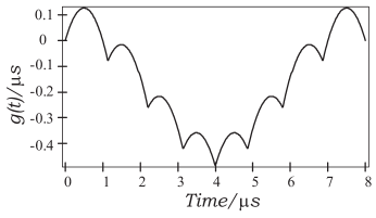
Figure 14: Visualization of the function $g(t)$ for $T_{R}=1\;\mu s$, $T_{S}=8\;\mu s$, $\Delta t=0.3\;\mu s$

As an abbreviation, we set

$$T_{k}=kT_{R}+\Delta t\;sin\left(2\pi k\frac{T_{R}}{T_{S}}\right)\mbox{\qquad}\Delta t<T_{R}/2$$

and

$$a_{k}(t)=t-T_{k}.$$

We define one period of a special periodic function by

$$g(t)=\frac{tT_{S}-t^{2}}{2T_{R}}+\sum_{k=1}^{\frac{T_{S}}{T_{R}}-1}\left[a_{k}(t)\sigma(a_{k}(t))-\frac{t}{T_{S}}a_{k}(T_{S})\right]$$

in the range $0\leq t\leq T_{S}$ ($g(t)=0$ elsewhere) such that the periodic function becomes

$$f^{(0)}(t)=\sum_{m=-\infty}^{+\infty}g(t-mT_{S}).$$

$\sigma(t)$ denotes the unit step function. An example for $g(t)$ is shown in Fig. 14. This function $f^{(0)}(t)$ is a continuous even function (note that $g(0)=g(T_{S})=0$). According to

$$a^{(p)}_{n}=\frac{2}{T_{S}}\int_{0}^{T_{S}}f^{(p)}(t)\;cos(n\omega_{S}t)\;dt$$

$$b^{(p)}_{n}=\frac{2}{T_{S}}\int_{0}^{T_{S}}f^{(p)}(t)\;sin(n\omega_{S}t)\;dt$$

we may derive the Fourier coefficients in order to get the series representation

$$f^{(p)}(t)=\frac{a^{(p)}_{0}}{2}+\sum_{n=1}^{\infty}a^{(p)}_{n}cos(n\omega_{S}t)+b^{(p)}_{n}sin(n\omega_{S}t).$$ (34)

A lengthy but straightforward calculation leads to

$$a^{(0)}_{n}=-\frac{2}{T_{S}(n\omega_{S})^{2}}\left[1+\sum_{k=1}^{\frac{T_{S}}{T_{R}}-1}cos\left(n\omega_{S}T_{k}\right)\right]\mbox{\quad for }n\neq 0,$$

$$a^{(0)}_{n}=\frac{T_{S}^{2}}{6T_{R}}+\sum_{k=1}^{\frac{T_{S}}{T_{R}}-1}\left(\frac{T_{k}^{2}}{T_{S}}-T_{k}\right)\mbox{\quad for }n=0,$$

$$b^{(0)}_{n}=0\mbox{\quad for all }n.$$

It is obvious that for $n\neq 0$,

$$|a^{(0)}_{n}|\leq\frac{2}{T_{R}(n\omega_{S})^{2}}$$

holds. Hence, we have $|a^{(0)}_{n}|<Mn^{\kappa}$ with real constants $M,\kappa$. According to (Zemanian, 1987), Corollary 2.4-3b, the series $f^{(p)}(t)$ in equation (34) converges in the space $\cal D^{\prime}$ of distributions. In $\cal D^{\prime}$ it is allowed to differentiate this series without further requirements ((Zemanian, 1987), Corollary 2.4-3a). For the function $g(t)$, we obtain

$$g^{\prime}(t)=\frac{T_{S}-2t}{2T_{R}}+\sum_{k=1}^{\frac{T_{S}}{T_{R}}-1}\left[\sigma(a_{k}(t))-\frac{1}{T_{S}}a_{k}(T_{S})\right]$$

(for $0<t<T_{S}$, $g^{\prime}(t)=0$ elsewhere). We find

$$g^{\prime}(0+) = 1-\frac{T_{S}}{2T_{R}}+\sum_{k=1}^{\frac{T_{S}}{T_{R}}-1}\frac{T_{k}}{T_{S}}$$

$$g^{\prime}(T_{S}-) = -\frac{T_{S}}{2T_{R}}+\sum_{k=1}^{\frac{T_{S}}{T_{R}}-1}\frac{T_{k}}{T_{S}}$$

such that

$$f^{(1)}(t)=\sum_{m=-\infty}^{+\infty}g^{\prime}(t-mT_{S})$$

(regarded as a locally integrable function) has unit steps at $t=mT_{S}$. Both $g^{\prime}$ and $f^{(1)}$ are locally integrable functions and may therefore be regarded as regular distributions.

As mentioned above, we may now differentiate this distribution. Thus we obtain in $\cal D^{\prime}$:

$$f^{(2)}(t)=-\frac{1}{T_{R}}+\sum_{k=-\infty}^{+\infty}\delta(a_{k}(t))$$

On the other hand, the derivative of eqn. (34) yields

$$f^{(2)}(t) = \sum_{n=1}^{\infty}a^{(2)}_{n}cos(n\omega_{S}t)=$$

$$= -\sum_{n=1}^{\infty}a^{(0)}_{n}(n\omega_{S})^{2}cos(n\omega_{S}t)$$

with

$$a^{(2)}_{n}=\frac{2}{T_{S}}\left[1+\sum_{k=1}^{\frac{T_{S}}{T_{R}}-1}cos\left(n\omega_{S}T_{k}\right)\right]\mbox{\quad for }n\neq 0.$$

This completes the proof of eqn. (29).