Abstract

Lowest-order cumulants provide important information on the shape of the emission source in femtoscopy. For the simple case of noninteracting identical particles, we show how the fourth-order source cumulant can be determined from measured cumulants in momentum space. The textbook Gram-Charlier series is found to be highly inaccurate, while the related Edgeworth series provides increasingly accurate estimates. Ordering of terms compatible with the Central Limit Theorem appears to play a crucial role even for nongaussian distributions.

Keywords: femtoscopy, Edgeworth series, correlations, interferometry

PACS Nos.: 13.85.Hd, 13.87.Fh, 13.85.-t, 25.75.Gz

1 Introduction

The large experimental statistics which are now available permit femtoscopic correlations of identical particles (see e.g. Ref.[1]) as a function of the full three-dimensional momentum difference ${\mathbf{q}}={\mathbf{p}}_{1}-{\mathbf{p}}_{2}$ and often also of the average pair momentum ${\mathbf{K}}=({\mathbf{p}}_{1}+{\mathbf{p}}_{2})/2$. Increasing attention has therefore been paid to the detailed description in these higher-dimensional spaces of the second-order correlation function

$$1+R({\mathbf{q}},{\mathbf{K}}) = C({\mathbf{q}},{\mathbf{K}})\ =\ \frac{\rho({\mathbf{q}},{\mathbf{K}})}{\rho^{\rm ref}({\mathbf{q}},{\mathbf{K}})},$$ (1)

with $\rho$ the density of like-sign pairs in sibling events and $\rho^{\rm ref}$ the reference pair density usually determined by a combination of event mixing and Monte Carlo simulation. After removing irrelevant correlations,[2] the correlation function can yield information on the spacetime statistical properties of particle emission as embodied in the source function $S({\mathbf{x}},{\mathbf{K}})$. The source function is obtained from the two-particle emission function, the density of particle emission points with near-equal momenta, by projection from the two four-coordinates onto the relative three-coordinate ${\mathbf{x}}$ (as measured in the pair rest frame of emission point densities)[3, 4, 5, 6]. The momentum- and coordinate-space correlations of noninteracting identical particles in their centre-of-mass system are related by a Fourier transform

$$R({\mathbf{q}},{\mathbf{K}})=\lambda\int d^{3}x\,S({\mathbf{x}},{\mathbf{K}})\,e^{i{\mathbf{q}}\cdot{\mathbf{x}}}\,,$$ (2)

where $\lambda$ is the correlation strength parameter. Suppressing the ${\mathbf{K}}$-dependence in a given global system, the two-particle correlation in both spaces can in this case be written as a normalised probability density function (pdf) $f({\mathbf{q}})$ in $q$-space and a pdf $g({\mathbf{x}})$ in $x$-space, related by

$$f({\mathbf{q}}) = \frac{R({\mathbf{q}})}{\int d^{3}q\,R({\mathbf{q}})}\ =\ f(\mathbf{0})\int d^{3}x\,e^{i{\mathbf{q}}\cdot{\mathbf{x}}}g({\mathbf{x}}),$$ (3)

$$g({\mathbf{x}}) = \frac{S({\mathbf{x}})}{\int d^{3}x\,S({\mathbf{x}})}\ =\ \int\frac{d^{3}q\,e^{-i{\mathbf{q}}\cdot{\mathbf{x}}}\,f({\mathbf{q}})}{(2\pi)^{3}f(\mathbf{0})}\ =\ \frac{S({\mathbf{x}})}{(2\pi)^{3}\,S(\mathbf{0})\,f(\mathbf{0})}\,.$$ (4)

A gaussian $f({\mathbf{q}})$ immediately yields a gaussian $g({\mathbf{x}})$ in any dimension. Experimental data, however, is often nongaussian, sometimes strongly so. This raises two problems: first, to systematically describe the nongaussian shape of $R$ (or $f$) in momentum space, and second, to determine parameters of $S$ (or $g$) in coordinate space, given only the kernel transform and measurements in $q$-space.

Approaches towards systematic description of nongaussian shapes in $q$-space can be found in e.g. Refs. [7, 8, 9], while the source function $S$ is reconstructed by means of higher-order coefficients in $x$-space using imaging techniques [10, 11, 12] and cartesian harmonics [2, 13].

In this paper, we wish to address the second problem of a systematic description of $g({\mathbf{x}})$ in terms of given measurements in $q$-space, based on the fundamental statistical properties of cumulants; the corresponding approach treating the first problem of measurements in $q$-space has been treated in part in the literature [14] [15] and will be more fully elaborated elsewhere.

2 Cumulants in dual spaces

While fully three-dimensional formulations have been in part set out in e.g. Ref. [15], we shall here work in one dimension using so that the above expressions become $g(x)=\int dq\,e^{-iqx}f(q)/2\pi f(0)$ and so on, our purpose being first to test and improve the convergence properties of series expansions in a simpler environment.

Given a measured normalised correlation function $f(q)$, its $q$-moments $\mu_{r}^{\scriptscriptstyle(q)}=\int dq\,f(q)\,q^{r}$ and $q$-cumulants $\kappa_{r}^{\scriptscriptstyle(q)}$ of lowest orders $r=1,2,3,\ldots$ provide fundamental information on its properties: the ordinary mean $\mu_{1}^{\scriptscriptstyle(q)}=\kappa_{1}^{\scriptscriptstyle(q)}=\int dq\,f(q)\,q$ is a measure of the location of the peak of $f(q)$, while the variance $\kappa_{2}^{\scriptscriptstyle(q)}=\mu_{2}^{\scriptscriptstyle(q)}-(\mu_{1}^{\scriptscriptstyle(q)})^{2}$ measures the dispersion and $\sigma=(\kappa_{2}^{\scriptscriptstyle(q)})^{1/2}$ the width or scale of the pdf, the skewness $\gamma_{3}^{\scriptscriptstyle(q)}=\kappa_{3}^{\scriptscriptstyle(q)}/\sigma^{3}$ measures its asymmetry and the kurtosis $\gamma_{4}^{\scriptscriptstyle(q)}=\kappa_{4}^{\scriptscriptstyle(q)}/\sigma^{4}$ is a first description of the pdf tail’s decay rate. Higher-order “generalised kurtoses” $\gamma_{r}^{\scriptscriptstyle(q)}=\kappa_{r}^{\scriptscriptstyle(q)}/\sigma^{r}$ would provide successively more detail. Kurtoses $\gamma_{r}^{\scriptscriptstyle(q)}$ can also be generally viewed as cumulants of the pdf $f(q^{\prime})$ of the standardised variable $q^{\prime}=(q-\mu_{1}^{\scriptscriptstyle(q)})/\sigma$.

Equivalent relations hold in coordinate space between $x$-moments, $x$-cumulants and $g(x)$, e.g. $\mu_{r}^{\scriptscriptstyle(x)}=\int dx\,g(x)\,x^{r}$, $\kappa_{2}^{\scriptscriptstyle(x)}=\mu_{2}^{\scriptscriptstyle(x)}-(\mu_{1}^{\scriptscriptstyle(x)})^{2}$ and so on.

$q$-moments are derivatives of the generating function $\Phi(x)=2\pi f(0)g(-x)=\int dq\,e^{iqx}f(q)$,

$$\mu_{r}^{\scriptscriptstyle(q)}=(-i)^{r}D_{x}^{r}\Phi(x)\bigr{|}_{x=0}\,,$$ (5)

writing $D_{x}^{r}=(d/dx)^{r}$ for short, while the related derivation of $q$-cumulants from

$$\kappa_{r}^{\scriptscriptstyle(q)}=(-i)^{r}D_{x}^{r}\ln\Phi(x)\bigr{|}_{x=0}$$ (6)

fixes relations between moments and cumulants to all orders. For identical particles, both $C({\mathbf{q}})=C(-{\mathbf{q}})$ and $g({\mathbf{x}})$ are symmetric, so that moments and cumulants of odd order vanish and the even-order relations in both $q$-space and $x$-space become

$$\kappa_{2} = \mu_{2},$$ (7)

$$\kappa_{4} = \mu_{4}-3\mu_{2}^{2},$$ (8)

$$\kappa_{6} = \mu_{6}-15\mu_{4}\mu_{2}+30\mu_{2}^{3}\qquad\text{etc.}$$ (9)

Cumulants form a natural basis for near-gaussian expansions since a gaussian pdf is fully determined once $\kappa_{1}$ and $\kappa_{2}$ are known: all its $\kappa_{r\geq 3}$ are identically zero. They also have important properties such as invariance under translation and a null result for uncorrelated variables.

While for purely gaussian sources, the second-order cumulants are related by $\kappa_{2}^{\scriptscriptstyle(x)}=1/\kappa_{2}^{\scriptscriptstyle(q)}$ and all higher-order cumulants are identically zero, neither of these statements is true in general. We will therefore consider both the modification of $\kappa_{2}^{\scriptscriptstyle(x)}$ resulting from nonzero $\gamma_{r}^{\scriptscriptstyle(q)}$ as well as the $x$-kurtosis $\gamma_{4}^{\scriptscriptstyle(x)}=\kappa_{4}^{\scriptscriptstyle(x)}/(\kappa_{2}^{\scriptscriptstyle(x)})^{2}$. Since $x$-moments are found from the generating function

$$\Phi(q)=f(q)\,/\,f(0)$$ (10)

through

$$\mu_{r}^{\scriptscriptstyle(x)}=(-i)^{r}D_{q}^{r}\Phi(q)\bigr{|}_{q=0}\,,$$ (11)

we can through Eqs. (7)–(9) obtain $x$-cumulants as combinations of measured $q$-moments.

3 Gram-Charlier expansions

3.1 Expressing $\gamma_{r}^{\scriptscriptstyle(x)}$ in terms of $\gamma_{r}^{\scriptscriptstyle(q)}$

While experimental measurement of derivatives of $\Phi(q)$ is of course impossible, the above expressions can nevertheless be evaluated since Gram-Charlier and Edgeworth series expansions also probe regions of nonzero $q$. Both expansions start with choosing a reference pdf $f_{0}(q)$ which, given the close relation between cumulants and gaussians, is almost invariably chosen by textbooks [16, 17] to be a gaussian

$$f_{0}(q)=\frac{e^{-q^{2}/2\sigma^{2}}}{\sigma\sqrt{2\pi}}\qquad\text{i.e.}\qquad f_{0}(q^{\prime})=\frac{e^{-q^{\prime 2}/2}}{\sqrt{2\pi}}$$ (12)

with the free parameter $\sigma^{2}$ fixed to the experimentally measured $\kappa_{2}^{\scriptscriptstyle(q)}$. The resulting “Gauss Gram-Charlier” (GGC) series, also known as the “Gram-Charlier Type A” series, and the corresponding Gauss Edgeworth (GEW) series are closely related, being mere re-orderings of one another, and are therefore commonly considered to be one and the same. As we will show, however, the GEW far outperforms the GGC series at any order of the partial sums.

As shown elsewhere,[18] the GGC series results from expanding the generating function for the nongaussian $f(q^{\prime})$ in powers of $x^{\prime}$

$$\Phi(x^{\prime})=e^{-x^{\prime 2}/2}\,\exp\biggl{[}\sum_{j=3}^{\infty}\zeta_{j}\,(ix^{\prime})^{j}\biggr{]}=e^{-x^{\prime 2}/2}\sum_{m=0}^{\infty}\frac{c_{m}(\bm{\zeta})}{m!}\,(ix^{\prime})^{m}$$ (13)

where each $c_{m}(\bm{\zeta})$ is a polynomial in the set of $q$-kurtoses $\bm{\zeta}=\{\zeta_{r}=\gamma_{r}^{\scriptscriptstyle(q)}/r!\}_{r=4}^{m}$. Taking the inverse Fourier transform of $\Phi(x^{\prime})$ term by term, one obtains an expansion in terms of Chebychev-Hermite polynomials $H_{r}(q^{\prime})$,

$$f(q^{\prime}) = f_{0}(q^{\prime})\biggl{[}1+\sum_{j=2}^{\infty}\frac{c_{2j}(\bm{\zeta})}{(2j)!}H_{2j}(q^{\prime})\biggr{]},$$ (14)

$$H_{r}(q^{\prime}) = f_{0}^{-1}(q^{\prime})\;(-D_{q^{\prime}})^{r}f_{0}(q^{\prime})\,,$$ (15)

with lowest-order terms (writing $H_{r}(q^{\prime})=H_{r}$ for short)

$$f(q^{\prime}) = f_{0}(q^{\prime})\biggl{[}1+\zeta_{4}H_{4}+\zeta_{6}H_{6}+\bigl{(}\zeta_{8}+\tfrac{1}{2}\zeta_{4}^{2}\bigr{)}H_{8}+\bigl{(}\zeta_{10}+\zeta_{6}\,\zeta_{4}\bigr{)}H_{10}$$ (16)

$$\qquad\qquad+\ \bigl{(}\zeta_{12}+\zeta_{8}\,\zeta_{4}+\tfrac{1}{2}\zeta_{6}^{2}+\tfrac{1}{6}\zeta_{4}^{3}\bigr{)}H_{12}\ +\ \ldots\biggr{]}.$$

Using $(-D_{q^{\prime}})^{r}f_{0}(q^{\prime})H_{2j}(q^{\prime})=f_{0}(q^{\prime})H_{2j+r}(q^{\prime})$, the $r$-th derivative of the $x$-moment generating function is, for even $r$,

$$\Phi^{(r)}(q^{\prime})=e^{-q^{\prime 2}/2}\left[H_{r}(q^{\prime})+\zeta_{4}H_{4+r}(q^{\prime})+\zeta_{6}H_{6+r}(q^{\prime})+\ldots\right],$$

from which the $x$-cumulants follow as ratios of generating functions at $q^{\prime}=0$ in terms of generalised $q$-kurtoses $\gamma_{r}=\kappa_{r}^{\scriptscriptstyle(q)}/\sigma^{r}$ and using $H_{2r}(0)=(-1)^{r}(2r-1)!!$

$$\kappa_{2}^{\scriptscriptstyle(x)} = \frac{(-i)^{2}}{\kappa_{2}^{\scriptscriptstyle(q)}}\frac{\Phi^{(2)}(q^{\prime})}{\Phi^{(0)}(q^{\prime})}\biggr{|}_{q^{\prime}=0}=\frac{1}{\kappa_{2}^{\scriptscriptstyle(q)}}\left[\frac{1+\tfrac{5}{8}\gamma_{4}-\tfrac{7}{48}\gamma_{6}+\tfrac{3}{128}(\gamma_{8}+35\gamma_{4}^{2})+\ldots}{1+\tfrac{1}{8}\gamma_{4}-\tfrac{1}{48}\gamma_{6}+\tfrac{1}{384}(\gamma_{8}+35\gamma_{4}^{2})+\ldots}\right]$$ (17)

while the $x$-kurtosis in fourth order is

$$\gamma_{4}^{\scriptscriptstyle(x)} = \frac{\Phi^{(4)}\,\Phi^{(0)}-3\Phi^{(2)}\,\Phi^{(2)}}{\Phi^{(2)}\,\Phi^{(2)}}\biggr{|}_{q^{\prime}=0}=\left[\frac{\gamma_{4}-\tfrac{1}{2}\gamma_{6}+\tfrac{1}{8}\gamma_{8}+\tfrac{15}{4}\gamma_{4}^{2}+\ldots}{1+\tfrac{5}{4}\gamma_{4}-\tfrac{7}{24}\gamma_{6}+\tfrac{3}{64}\gamma_{8}+\tfrac{65}{32}\gamma_{4}^{2}+\ldots}\right]$$ (18)

with a similar expression for $\kappa_{4}^{\scriptscriptstyle(x)}$.

Note firstly that $\gamma_{4}^{\scriptscriptstyle(x)}$ depends only on $\gamma_{r}^{\scriptscriptstyle(q)}$ but not directly on $\sigma^{2}=\kappa_{2}^{\scriptscriptstyle(q)}$; this is true also for higher-order $\gamma_{r}^{\scriptscriptstyle(x)}$. Secondly, the above relations reduce to the gaussian relation $\kappa_{2}^{\scriptscriptstyle(x)}=1/\kappa_{2}^{\scriptscriptstyle(q)}$ and $\gamma_{4}^{\scriptscriptstyle(x)}=0$ if and when the measured correlation function is gaussian since as mentioned all $\gamma_{r\geq 3}^{\scriptscriptstyle(q)}$ are then identically zero. In general, however, the “radius” $[2\kappa_{2}^{\scriptscriptstyle(x)}]^{1/2}$ of the source distribution is a function also of higher-order $q$-cumulants, with both increasing orders $\gamma_{r}^{\scriptscriptstyle(q)}$ and increasing powers of lower-order $\gamma_{r}^{\scriptscriptstyle(q)}$ entering the expansions.

Given the symmetry between $x$ and $q$, the corresponding expansions for $\kappa_{2}^{\scriptscriptstyle(q)}$ and $\gamma_{r}^{\scriptscriptstyle(q)}$ in terms of $\kappa_{2}^{\scriptscriptstyle(x)}$ and $\gamma_{r}^{\scriptscriptstyle(x)}$ would have the same form as the above, apart from some changes in sign. Any measured $\kappa_{2}^{\scriptscriptstyle(q)}$ is therefore itself the result of contributions from higher-order cumulants of $g(x)$ or, in physics terms, the nongaussian shape of the emission region.

3.2 Truncation and the GGC disaster

Statistical errors on $q$-cumulants rise with increasing order so that only those lower-order ones accessible to available experimental statistics can be included. Series expansions such as (14) are known to be asymptotic, so that the question arises: how accurately can a series truncated at some maximum order $\gamma_{r{\rm max}}$ and/or a maximum power $\gamma_{r}^{k{\rm max}}$ estimate the $\gamma_{r}^{\scriptscriptstyle(x)}$?

To quantify this issue, we make use of the Normal Inverse Gaussian (NIG) probability density [19] as a solvable toy model for $f(q^{\prime})$ which yields exact expressions for both coordinate- and momentum-space cumulants. While the NIG has four parameters $\alpha$, $\beta$, $\mu$ and $\delta$, in the present symmetric case $\beta=\mu=0$, so that we need only the two-parameter Symmetric Normal Inverse Gaussian (SNIG),

$$f(q\,|\,\alpha,\delta)=\frac{\alpha\delta\,e^{\alpha\delta}\,K_{1}(\alpha\sqrt{\delta^{2}+q^{2}})}{\pi\sqrt{\delta^{2}+q^{2}}}\,,$$ (19)

where $K_{1}$ is the modified Bessel function. The SNIG reverts to a gaussian in the limit $\alpha\to\infty$ and has $q$-moment generating function $\Phi(x\,|\,\alpha,\delta)=\exp[\delta\alpha-\delta\sqrt{\alpha^{2}+x^{2}}]$. Experimentally measured $\kappa_{2}^{\scriptscriptstyle(q)}$ and $\gamma_{4}^{\scriptscriptstyle(q)}$ would fix the parameters: writing $\sigma=[\kappa_{2}^{\scriptscriptstyle(q)}]^{1/2}$ and $g=\gamma_{4}^{\scriptscriptstyle(q)}$ for short, $\alpha=[3/g\sigma^{2}]^{1/2}$ and $\delta=[3\sigma^{2}/g]^{1/2}$, so that higher-order cumulants and kurtoses can be expressed in terms of measured quantities $\sigma$ and $g$ as

$$\kappa_{r,\scriptscriptstyle{\rm SNIG}}^{\scriptscriptstyle(q)} = (r-1)!!\,(r-3)!!\;\sigma^{r}\,[\tfrac{1}{3}\,g]^{\tfrac{r}{2}-1}\,,$$ (20)

$$\gamma_{r,\scriptscriptstyle{\rm SNIG}}^{\scriptscriptstyle(q)} = (r-1)!!\,(r-3)!!\;[\tfrac{1}{3}\,g]^{\tfrac{r}{2}-1}.$$ (21)

Using the SNIG pdf as $x$-moment generating function in the form (10)

$$\Phi(q\,|\,\alpha,\delta)=\frac{K_{1}(\alpha\sqrt{q^{2}+\delta^{2}})}{K_{1}(\alpha\delta)}\cdot\frac{\delta}{\sqrt{q^{2}+\delta^{2}}}$$

we obtain exact expressions for $x$-cumulants via (11) and the moment-cumulant relations. Omitting the argument of the Bessel functions, which is $\alpha\delta=3/g$ in every case, these “exact” $x$-cumulants are

$$\kappa_{2,\scriptscriptstyle{\rm SNIG}}^{\scriptscriptstyle(x)} = \frac{1}{\kappa_{2}^{\scriptscriptstyle(q)}}\cdot\frac{K_{2}}{K_{1}}\,,$$ (22)

$$\kappa_{4,\scriptscriptstyle{\rm SNIG}}^{\scriptscriptstyle(x)} = \frac{1}{\kappa_{2}^{{\scriptscriptstyle(q)}\,2}}\cdot\frac{3K_{3}K_{1}-3K_{2}^{2}}{K_{1}^{2}}\,,$$ (23)

$$\gamma_{4,\scriptscriptstyle{\rm SNIG}}^{\scriptscriptstyle(x)} = \frac{3K_{3}K_{1}-3K_{2}^{2}}{K_{2}^{2}}\,.$$ (24)

With these exact $x$-cumulants as reference, we test the accuracy of various truncations of Eqs. (17)–(18) as a function of the Gram-Charlier order $m=2j$ of Eq. (14).

The results are disastrous. In Fig. 1, we show respectively the percentage deviation of GGC expansions (17) and (18), truncated at $m$th order, from the exact answers (22) and (24), in the form $100(\kappa_{2,m}^{\scriptscriptstyle(x)}/\kappa_{2,\scriptscriptstyle{\rm SNIG}}^{\scriptscriptstyle(x)}-1)$ and $100(\gamma_{4,m}^{\scriptscriptstyle(x)}/\gamma_{4,\scriptscriptstyle{\rm SNIG}}^{\scriptscriptstyle(x)}-1)$. At $\gamma_{4}^{\scriptscriptstyle(q)}=0$, of course, all series reduce to a gaussian and all approximations become exact. Even small values of $\gamma_{4}^{\scriptscriptstyle(q)}$ lead to large deviations, however, and the size of the deviations increases with order $m$. GGC series fail completely to approximate the exact $x$-cumulants.

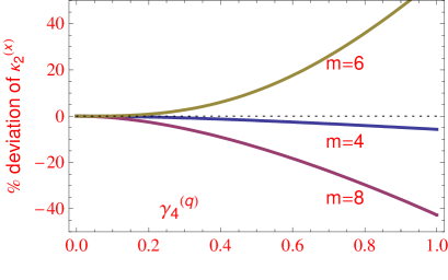
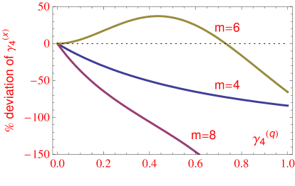
Figure 1: Gauss Gram-Charlier series fail badly: Percentage deviations of Gram-Charlier approximations of $\kappa_{2}^{\scriptscriptstyle(x)}$ found by Eq. (17) vs. (22) and of $\gamma_{4}^{\scriptscriptstyle(x)}$ found by (18) vs. (24), as a function of the measured $q$-kurtosis $\gamma_{4}^{\scriptscriptstyle(q)}$ for various Gram-Charlier orders $m$.

4 Edgeworth series

4.1 Derivation and properties

In his 1946 treatise on statistics, Cramér[20] derived the Gauss-Edgeworth (GEW) series by considering the random variable ($q^{\prime}$ in our case) to be a convolution of $n$ identically-distributed independent (iid) random variables $q_{i}$ each with pdf $f_{1}(q_{i})$, a corresponding generating function $\Phi_{1}(x_{i})$ and second-order cumulant $\kappa_{2}^{\scriptscriptstyle(q)}(n{=}1)=\sigma_{1}^{2}$, in terms of which the generating function for $x^{\prime}$, the dual to $q^{\prime}=\sum_{i}q_{i}/(\sigma_{1}\sqrt{n})$, is

$$\Phi(x^{\prime})=\prod_{i=1}^{n}\int dq_{i}\,f_{1}(q_{i})\,\exp\!\left[\frac{iq_{i}x^{\prime}}{\sigma_{1}\sqrt{n}}\right]=\left[\Phi_{1}\left(\frac{x^{\prime}}{\sigma_{1}\sqrt{n}}\right)\right]^{n}\,.$$ (25)

For such convolutions, cumulants of $f(q^{\prime})$ are related to cumulants of $f(q_{i})$ by $\kappa_{j}^{\scriptscriptstyle(q)}(n)=n\,\kappa_{j}^{\scriptscriptstyle(q)}(1)$, so that

$$\zeta_{j}(n)=\frac{\zeta_{j}(1)}{n^{\tfrac{j}{2}-1}}\,.$$ (26)

and hence $\Phi(x^{\prime})$ depends on $\ell=n^{-1/2}$ through

$$\Phi(x^{\prime})=e^{-x^{\prime 2}/2}\exp\biggl{[}\,\sum_{j=3}^{\infty}(ix^{\prime})^{j}\,\zeta_{j}(n)\biggr{]}\ =\ e^{-x^{\prime 2}/2}\exp\biggl{[}\,\sum_{j=3}^{\infty}(ix^{\prime})^{j}\,\zeta_{j}(1)\,\ell^{j-2}\biggr{]}.$$ (27)

Expanding the exponential in powers of $\ell$ rather than of $x^{\prime}$ and again inverting term by term, we obtain the Gauss-Edgeworth series

$$f(q^{\prime}) = f_{0}(q^{\prime})\biggl{[}1+\ell^{2}\zeta_{4}H_{4}+\ell^{4}\left(\tfrac{1}{2}\zeta_{4}^{2}H_{8}+\zeta_{6}H_{6}\right)+\ell^{6}\left(\tfrac{1}{6}\zeta_{4}^{3}H_{12}+\zeta_{4}\zeta_{6}H_{10}+\zeta_{8}H_{8}\right)$$ (28)

$$\quad+\ell^{8}\left(\tfrac{1}{24}\zeta_{4}^{4}H_{16}+\tfrac{1}{2}\zeta_{4}^{2}\zeta_{6}H_{14}+\tfrac{1}{2}\zeta_{6}^{2}H_{12}+\zeta_{4}\zeta_{8}H_{12}+\zeta_{10}H_{10}\right)\ +\ \ldots\biggr{]},$$

again writing $H_{r}=H_{r}(q^{\prime})$ for short and with $\zeta_{j}$ here understood as $\zeta_{j}(1)$. Unlike the equivalent GGC expansion of Eq. (16), in which the order of the expansion was determined by the order of $H_{m}$, a given term of order $\ell^{w}$ in the GEW series is a linear combination of Hermite polynomials of different order.

The relation between Gram-Charlier and Edgeworth ordering is summarised in Table 1, with terms listed in ascending order for $w$. A given term $\zeta_{r_{1}}\zeta_{r_{2}}\!\cdots$ is characterised by the set of partition coefficients $r_{k}=4,6,8,\ldots$ which are constrained to the Gram-Charlier and Edgeworth orders by

$$\sum_{k}r_{k} = m\,,$$ (29)

$$\sum_{k}(r_{k}-2) = w\,.$$ (30)

The re-ordering becomes important already for the second-lowest order $w=4$.

series		Edgeworth	Gram-Charlier
term	$\{r_{k}\}\quad$	order $w$	order $m$
$\zeta_{4}$	$\{4\}$	2	4
$\zeta_{6}$	$\{6\}$	4	6
$\zeta_{4}^{2}$	$\{4,4\}$	4	8
$\zeta_{8}$	$\{8\}$	6	8
$\zeta_{6}\zeta_{4}$	$\{6,4\}$	6	10
$\zeta_{4}^{3}$	$\{4,4,4\}$	6	12
$\zeta_{10}$	$\{10\}$	8	10
$\zeta_{6}^{2}$	$\{6,6\}$	8	12
$\zeta_{8}\zeta_{4}$	$\{8,4\}$	8	12
$\zeta_{6}\zeta_{4}^{2}$	$\{6,4,4\}$	8	14
$\zeta_{4}^{4}$	$\{4,4,4,4\}$	8	16

Table 1: Re-ordering of terms between Gram-Charlier (GC) and Edgeworth (EW) series

4.2 Test using SNIG

Edgeworth re-ordering of terms in the derivatives $\Phi^{(r)}(q^{\prime})$ leads to expressions for the $x$-cumulants as ratios of power series in $\ell$. For the SNIG test case, these series simplify to

$$\kappa_{2}^{\scriptscriptstyle(x)} = \frac{1}{\kappa_{2}^{\scriptscriptstyle(q)}}\left[\frac{1+\frac{5}{8}\gamma_{4}\ell^{2}+\frac{35}{384}\gamma_{4}^{2}\ell^{4}-\frac{35}{3072}\gamma_{4}^{3}\ell^{6}+\frac{385}{98304}\gamma_{4}^{4}\ell^{8}+\ldots}{1+\frac{1}{8}\gamma_{4}\ell^{2}-\frac{5}{384}\gamma_{4}^{2}\ell^{4}+\frac{35}{9216}\gamma_{4}^{3}\ell^{6}-\frac{175}{98304}\gamma_{4}^{4}\ell^{8}+\ldots}\right],$$ (31)

$$\gamma_{4}^{\scriptscriptstyle(x)} = \qquad\left[\frac{\gamma_{4}\ell^{2}+\frac{5}{4}\gamma_{4}^{2}\ell^{4}+\frac{35}{96}\gamma_{4}^{3}\ell^{6}-\frac{35}{1152}\gamma_{4}^{4}\ell^{8}+\ldots}{1+\frac{5}{4}\gamma_{4}\ell^{2}+\frac{55}{96}\gamma_{4}^{2}\ell^{4}+\frac{35}{384}\gamma_{4}^{3}\ell^{6}+\frac{35}{18432}\gamma_{4}^{4}\ell^{8}+\ldots}\right]\,,$$ (32)

with $\gamma_{4}\equiv\gamma_{4}^{\scriptscriptstyle(q)}(1)$. The algebraic simplicity of the above compared to the equivalent GGC relations (17)–(18) and the GEW relation (28) is due to the fact that SNIG kurtoses obey

$$\gamma_{j}^{\scriptscriptstyle(q)}=F_{j}\,[\gamma_{4}^{\scriptscriptstyle(q)}]^{\tfrac{j}{2}-1}$$ (33)

with constants $\{F_{4},F_{6},F_{8},\ldots\}=\{1,5,\tfrac{175}{3},\ldots\}$ fully determined by the SNIG pdf. While relation (33) is of course fulfilled by all convolutions through (26), it is true for the SNIG case even without convolution.

In Fig. 2, we show the percentage deviations of the Edgeworth-truncated approximations (31)–(32) from their respective exact SNIG values as a function of the $q$-kurtosis $\gamma_{4}^{\scriptscriptstyle(q)}$. The improvement in accuracy over the GGC ordering is dramatic. Unlike the GGC, the GEW series also continues to improve as higher orders of $w$ are included.

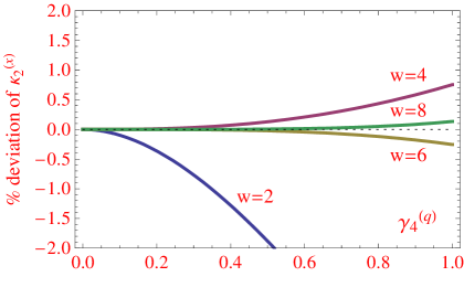
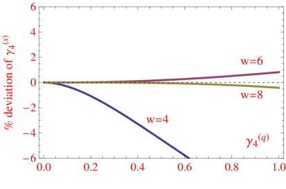
Figure 2: Gauss Edgeworth series: Percentage deviations of GEW approximations of $\kappa_{2}^{\scriptscriptstyle(x)}$ found by Eq. (31) vs. (22) and of $\gamma_{4}^{\scriptscriptstyle(x)}$ found by (32) vs. (24), as a function of the $q$-kurtosis $\gamma_{4}^{\scriptscriptstyle(q)}$ for various Edgeworth orders $w$. The dashed line at zero marks perfect agreement between the truncated expansion and the exact SNIG answer.

4.3 $n$-divisibility and the Central Limit Theorem

What structure or principle underlies the strong superiority of GEW over GGC ordering? Clearly, the expansion parameter $n=\ell^{-2}$ must be playing a crucial role. Eq. (25) characterises the generating function $\Phi(x^{\prime})$ and therefore the pdf $f(q^{\prime})$ as “$n$-divisible” or more prosaically as precisely that convolution $f(q^{\prime})=\delta[q^{\prime}-\sum_{i}q_{i}/\sigma_{1}\sqrt{n}\,]\,\prod_{i}f(q_{i})$ which led to Eq. (25). The GEW method might therefore be expected to work well if $n$-divisibility could be established for a given experimental data set. However, it is usually not possible to directly establish whether the $f(q^{\prime})$ of an experimental data set is $n$-divisible, and there is no obvious physics reason to believe that a momentum difference $q^{\prime}$ between two particles is the result of an underlying summation.

The reason for the success of GEW relies not on physics assumptions, but on a better description of nongaussian systems. In statistics terms, any deviation from the gaussian is captured by the GEW series in the rate of approach of higher-order cumulants to zero with increasing $n$. Indeed, many proofs of the Central Limit Theorem rely on the fact that $\kappa_{j}(n)=n\,\kappa_{j}(1)$ immediately yields the fixed rate of convergence for any generalised kurtosis as shown in Eq. (26).

The success of GEW ordering is therefore based on the fact that all contributing terms in a given order of $\ell=n^{-1/2}$ have the same rate of convergence to the gaussian limit. Furthermore, due to the alternating sign of $H_{2r}(0)=(-1)^{r}(2r-1)!!$, the sum of contributions within a given $O(\ell^{w})$ term tends to be substantially smaller than the individual contributions; for example the $w=4$ term for the SNIG test case is made up of $\tfrac{1}{2}\zeta_{4}^{2}H_{8}(0)=0.091\gamma_{4}^{2}$ and $\zeta_{6}F_{6}H_{6}(0)=-0.104\gamma_{4}^{2}$, adding up to $-0.013\gamma_{4}^{2}$.

It is not necessary to know the value of $n$ to make use of GEW ordering: Using (26), we can merely re-absorb the $\ell^{w}$ in (28) to write the GEW expansion in $n$-independent notation (now with $\zeta_{j}\equiv\zeta_{j}(n)$, the measured kurtosis)

$$f(q^{\prime}) = f_{0}(q^{\prime})\biggl{[}1+\bigl{(}\zeta_{4}H_{4}\bigr{)}+\left(\tfrac{1}{2}\zeta_{4}^{2}H_{8}+\zeta_{6}H_{6}\right)+\left(\tfrac{1}{6}\zeta_{4}^{3}H_{12}+\zeta_{4}\zeta_{6}H_{10}+\zeta_{8}H_{8}\right)$$ (34)

$$\quad+\left(\tfrac{1}{24}\zeta_{4}^{4}H_{16}+\tfrac{1}{2}\zeta_{4}^{2}\zeta_{6}H_{14}+\tfrac{1}{2}\zeta_{6}^{2}H_{12}+\zeta_{4}\zeta_{8}H_{12}+\zeta_{10}H_{10}\right)\ +\ \ldots\biggr{]},$$

but keeping in mind that each expression within a round bracket represents a certain rate of convergence and must be included or excluded as a whole.

It is not even necessary to require $n$-divisibility as such: For the GEW ordering to be effective we require only that $f(q)$ is reasonably close to a gaussian, where “reasonable” is typically quantified by the errors shown in Fig. 2. The derivation also does not rely on a particular form of $f_{1}(q_{i})$ other than requiring existence of its cumulants.

5 Conclusions

We have calculated expressions for $x$-cumulants of second and fourth order for the emission region in terms of measured $q$-cumulants. On using a nongaussian test function to quantify accuracy of expansions, we have shown that the textbook Gram-Charlier series is unsuitable at any level of approximation. By contrast, the Gauss-Edgeworth expansion, which orders terms based on the rate of approach to a gaussian, does give results which become increasingly accurate as more terms are added. The GEW series is robust in all respects; for example it does not require $n$-divisibility as such but only that $f(q)$ be close enough to a gaussian in the sense that the measured $q$-cumulants entering truncated GEW expansion should have reasonable error bars.

The present one-dimensional calculation clearly cannot be applied immediately to experimental data, but is meant to show that, even on the fundamental level of expansions, there are major questions which must be addressed first. In sorting out the fundamental issue of re-ordering, the present results represent an important step towards a consistent framework for shape description.

Application to experimental data will require generalisation to three dimensions using the existing 3D machinery of Refs [15, 18]. Furthermore, sampling fluctuations of experimental cumulants will have to be taken into account. In this connection, we also note that the GEW ordering has the additional advantage of placing terms with higher powers of $\gamma_{4}^{\scriptscriptstyle(q)}$ into lower orders of $w$, making it unnecessary to measure higher-order kurtoses. Based on slightly different arguments, Cramér [20] also concluded that GEW was superior to GGC ordering; this has also been verified GGC vs GEW comparisons of the nongaussian pdf itself [21, 22]. The Gram-Charlier series can therefore be considered to be inferior to the Edgeworth equivalent in all respects.

Note that it is not necessary to measure the correlation function $f(q)$ at $q=0$, despite the fact that $x$-cumulants rely formally on the generating function (11) at zero. The $q$-cumulants themselves are functions of $f(q)$ over the whole range of $q$, while the correlation strength parameter $\lambda$ cancels in the normalisation (3).

Our final comment pertains to the usual practice of obtaining information on the correlation function through fits of nongaussian parametrisations. Fits rely on an a priori choice of parametrisation, guided only by the minimisation of $\chi^{2}$, and suffer from increasing ambiguity in higher dimensions. By relying on direct measurement of coefficients, the present method and those of Refs [11, 12] etc leave less room for arbitrary choices and put the uncertainty where it belongs: in the sampling fluctuations of measured experimental quantities.

Acknowledgements: This work was supported in part by the National Research Foundation of South Africa.

References

• [1] M.A. Lisa, S. Pratt, R. Soltz and U.A. Wiedemann, Ann. Rev. Nucl. Part. Sci. 55, 357 (2005).
• [2] STAR Collaboration, M.M. Aggarwal et al., arXiv:1004.0925 (2010).
• [3] S. Pratt, Phys. Rev. Lett. 53, 1219 (1984).
• [4] S.V. Akkelin et al., Phys. Rev. C 65, 064904 (2002); nucl-th/0107015.
• [5] R. Lednicky, Braz. J. Phys. 37, 939 (2007); nucl-th/0702063.
• [6] P. Danielewicz and S. Pratt, Phys. Rev. C 75, 034907 (2007).
• [7] S. Hegyi and T. Csörgő, Proc. Budapest Workshop on Relativistic Heavy Ion Collisions, preprint KFKI-1993-11/A, (1994).
• [8] T. Csörgő and S. Hegyi, Phys. Lett. B 489, (2000).
• [9] Z. Chajecki, T.D. Gutierrez, M.A. Lisa and M. Lopez-Noriega, in: Proc. 21st Winter Workshop on Nuclear Dynamics, Eds. R. B. W. Bauer and S. Panitkin, EP Systems, Budapest (2005), pp. 3205–3223.
• [10] D.A. Brown and P. Danielewicz, Phys. Lett. B 398, 252 (1997).
• [11] D.A. Brown and P. Danielewicz, Phys. Rev. C 57, 2474 (1998).
• [12] D.A. Brown, A. Enokizono, M. Heffner, R. Soltz, P. Danielewicz and S. Pratt, Phys. Rev. C 72, 054902 (2005).
• [13] P. Danielewicz and S. Pratt, Phys. Lett. B 618, 60 (2005).
• [14] U.A. Wiedemann and U. Heinz, Phys. Rev. C 56, R610 (1997).
• [15] H.C. Eggers and P. Lipa, Int. J. Mod. Phys. E 16, 3205 2007.
• [16] A. Stuart and J.K. Ord, Kendall’s Advanced Theory of Statistics, Volume1, 5th edition, Oxford University Press, New York (1987).
• [17] P. McCullagh, Tensor Methods in Statistics, Cambridge University Press (1987)
• [18] H.C. Eggers and P. Lipa, Braz. J. Phys., 37(3a), 877 (2007).
• [19] O.E. Barndorff-Nielsen, Scand. J. Statist., 24, 1 (1997).
• [20] H. Cramér, Mathematical Methods of Statistics, Princeton Mathematical Series Vol 9, Princeton University Press, 1946.
• [21] S. Blinnikov and R. Moessner, Astr. Astroph. Suppl. 130, 193 (1998).
• [22] M.B. de Kock, MSc Thesis, University of Stellenbosch (2009).