Interaction anisotropy and random impurities effects on the critical behaviour of ferromagnets

Abstract

The theory of phase transitions is based on the consideration of "idealized" models, such as the Ising model: a system of magnetic moments living on a cubic lattice and having only two accessible states. For simplicity the interaction is supposed to be restricted to nearest–neighbour sites only. For these models, statistical physics gives a detailed description of the behaviour of various thermodynamic quantities in the vicinity of the transition temperature. These findings are confirmed by the most precise experiments. On the other hand, there exist other cases, where one must account for additional features, such as anisotropy, defects, dilution or any effect that may affect the nature and/or the range of the interaction. These features may have impact on the order of the phase transition in the ideal model or smear it out. Here we address two classes of models where the nature of the transition is altered by the presence of anisotropy or dilution.

To appear in Journal of Physics: Conference Series

1 Introduction

Materials in Nature can be found in qualitatively different phases having distinct properties. The change from one phase to another is the consequence of a variation of an intensive thermodynamic quantity, e.g., the temperature $T$, the pressure $P$, external electric or magnetic fields $E$ or $H$. Phase transitions are accompanied by abrupt changes in a number of macroscopic thermodynamic quantities. Some familiar examples of phase transitions include the gas–liquid transition (condensation), the liquid–solid transition (freezing), the normal–superconducting transition in conductors, the paramagnet–ferromagnet transition in magnetic materials, and the superfluid transition in liquid helium. Further examples are transitions involving amorphous or glassy structures, spin glasses, liquid crystals, charge–density waves, and spin–density waves.

In many cases, the two phases above and below the transition point, say $T_{c}$ for a temperature driven phase transition, may be discerned from each other in terms of some ordering that occurs in the phase below $T_{c}$. For example in the liquid–solid transition the molecules of the liquid get “ordered” in space when they form the solid phase. In a paramagnet, the magnetic moments of each atom can point in any random direction (in the absence of an external magnetic field), but in the ferromagnetic phase the moments are lined up in a particular direction of ordering. Thus in the high temperature phase (above $T_{c}$), the degree of ordering is smaller than in the low temperature phase (below $T_{c}$). To quantify the amount of ordering in a system one uses the so called order parameter, which is usually a vanishing quantity in the high temperature (disordered) phase.

The phase diagram shows regions within which homogeneous equilibrium states exist as a function of temperature and other thermodynamic variables like $P$, $E$, $H$. For some physical systems the chemical potential $\mu$ or composition variables are also involved. The different regions of the phase diagram are delimited by phase boundaries that mark conditions under which multiple phases can coexist at equilibrium. Phase transitions take place along phase boundaries marked by lines of equilibrium.

The theoretical framework that aims at describing phase transitions and related phenomena as a result from cooperative effects over macroscopic scales is a part of the realm of equilibrium statistical physics [1, 2, 3]. Statistical physics is based on probabilistic models of the interactions of microscopic entities forming large assemblages (macroscopic bodies). The probability a macroscopic system of volume $V$, having $N$ particles, in a state $\mathfrak{S}$ with energy $E$ at a temperature $T$, is given by

$$\mathscr{P}(\mathfrak{S})=\frac{e^{-E(\mathfrak{S})/(k_{B}T)}}{\mathscr{Z}(T)},$$ (1)

where $k_{B}$ is the Boltzmann constant, and $\mathscr{Z}(T)$ is the partition function

$$\mathscr{Z}(T)=\sum_{\mathfrak{S}}e^{-E(\mathfrak{S})/(k_{B}T)},$$ (2)

relating microscopic degrees of freedom to macroscopic thermodynamic quantities. The function $\mathscr{Z}(T)$ depends upon any parameters that might affect the value of $E(\mathfrak{S})$. The expectation value of any statistical operator $\mathfrak{O}$ is defined via

$$\langle\mathfrak{O}(\mathfrak{S})\rangle=\sum_{\mathfrak{S}}\mathfrak{O}(\mathfrak{S})\mathscr{P}(\mathfrak{S}).$$ (3)

For example the internal energy $U$ is obtained by averaging $E(\mathfrak{S})$ over all the accessible states of the system. This is given by

$$U=\langle E(\mathfrak{S})\rangle.$$

A fundamental thermodynamic quantity related to the partition function is the free energy

$$f(T)=-k_{B}T\ln\mathscr{Z}(T),$$ (4)

which contains all the information on the thermodynamics of the considered system.

According to the Ehrenfest classification scheme there are different kinds of phase transitions depending on the nature of the singularities of the thermodynamic quantities at the transition. Such transitions are categorized as first–, second–, or higher order transitions if the lowest derivative of the free energy that exhibit nonanalytic behaviour with a finite jump is the first, second or higher one. Within this classification the Berezinskiǐ–Kosterlitz–Thouless (BKT) [4, 5] may be considered as being of infinite order.

To describe universal features of phase transitions one uses relatively “simple” microscopic models such as the magnetic model involving interaction between magnetic degrees of freedom. In a classical model for a magnet, the spins (magnetic moments) may be represented by $n$–component unit vectors $\bm{s}_{i}$ located at sites $i$, with coordinates $\bm{x}_{i}$, belonging to a finite subset of a generic $d$–dimensional lattice $\Lambda_{d}$, i.e. $\mathfrak{L}\subset\Lambda_{d}$, with $|\mathfrak{L}|=N$. We are considering here saturated lattice models, where each lattice site hosts one spin. The simplest and probably most extensively studied cases considered in the literature assume a hypercubic lattice $\Lambda_{d}=\mathbb{Z}^{d}$ and isotropically interacting spins, thus the (nearest–neighbour) Hamiltonian

$$\mathscr{H}_{\mathfrak{L}}=-\frac{J}{2}\sum_{\langle i,j\rangle}\bm{s}_{i}\cdot\bm{s}_{j}-\bm{H}\sum_{i}\bm{s}_{i},$$ (5)

where the coupling $J$ is restricted to nearest–neighbouring sites $i$ and $j$, with each distinct pair being counted once. $\bm{H}$ stands for an uniform magnetic field.

In the absence of the magnetic field, i.e. $\bm{H}=\bm{0}$, a ferromagnetic coupling, $J>0$, favours a parallel orientation of the spins in the ground state, whereas thermal fluctuations tend to create an orientational disorder. On the other hand an interaction, $J<0$, would be the precursor of an antiferromagnetic order at low temperatures. Actually, in the specific case considered here, i.e. nearest–neighbour coupling and bipartite lattice, and with $\bm{H}=\bm{0}$, the sign of the coupling constant is immaterial, i.e. models defined by $+J$ and $-J$ yield the same partition function, whereas the two correlation functions are connected by suitable sign factors.

For $n=1,2,3$, the model corresponds to the Ising, planar rotator (PR) and Heisenberg (He), respectively. The Ising model is known to have a $Z_{2}$ discrete symmetry, while systems with $n\geq 2$, like PR and He, are said to possess a continuous $O(n)$ symmetry. It has become customary to refer to the number of component $n$ of the order parameter as symmetry index. The interaction with an external field breaks this symmetry and establishes a preferred direction for spin alignment. By reducing the external field to zero in the thermodynamic limit, the system may exhibit spontaneous magnetization pointing in the initial direction of the field. It has been shown [6] that the limit $n\to\infty$ leads to the spherical model [7] obtained by requiring the spins to be continuous variables subject to a global relaxed constraint ($\sum_{i=1}^{N}\bm{s}_{i}^{2}=N$) rather than forcing them to take unit lengths i.e. $|\bm{s}_{i}|^{2}=1$. The formal limit $n\to 0$ is relevant to the study of self–avoiding walk problem, which can be applied to polymers.

By now a number of rigorous results, assuming translational invariance, have been worked out, entailing existence or absence of a phase transition in the thermodynamic limit, depending on lattice dimensionality $d$ and number of spins components $n$ [8, 9].

Model (5) with different values of $n$ and $d$ is extensively studied in the literature via different methods and its behaviour as a function of the temperature is very well known. For a review with a rich list of references see [10]. At $H=0$, it exhibits a second order phase transition, for any $d>1$ and with discrete spin variables, i.e. $n=1$. Such a transition is characterized by a significant growth of the nearest–neighbour correlations for orientational fluctuations, and also the onset for long–range orientational correlations. On the other hand, according to the Mermin–Wegner theorem [11] in $O(n)$ symmetric models ($n\geq 2$) there can be no spontaneous symmetry breaking at finite temperatures for $d\leq 2$ meaning that the system remains orientationally disordered at any finite temperature. For $d>2$ and $n\geq 2$ a second order phase transition takes place in the system. In the two–dimensional case $d=2$ and $n=2$ the system exhibits a BKT transition from a high temperature disordered phase to a low temperature phase with slow decay of the correlation function and an infinite magnetic susceptibility [12].

In the vicinity of a continuous phase transition, such as second order or BKT transition, there is only one dominating length scale related to the growth of fluctuations: The correlation length. Because of the diverging nature of the correlation length as the critical point is approached the microscopic details of the system becomes irrelevant. Thus the description of the singular behaviour of many thermodynamic observables requires a small number of universal variables: critical exponents, amplitudes and functions. This allows the arrangement of a great variety of different microscopic systems in universality classes of equivalent critical behaviour. A universality class depends upon the number of components of the order parameter and the dimensionality of the system. For more details the reader is invited to consult references [13, 14].

The model (5) can describe the properties of a wide variety of physical situations in the vicinity of their transition point, however, it may happen that the very experimental situation at hand requests the interaction model to be complicated (made physically richer and theoretically more challenging) in various ways. On the one hand, there exist different possible lattice types $\Lambda_{d}$, in addition to $\mathbb{Z}^{d}$. On the other hand, as for the orientational dependence, more elaborate potential models involve (in some combination or other) isotropic or anisotropic linear couplings between spin components, sometimes higher powers of scalar products among the interacting spins, multipolar (usually dipolar) interactions, Dzyaloshinski–Moriya terms, single–site anisotropy fields. Notice also that more distant neighbours are sometimes involved, or even, in principle, all neighbours may be coupled by long–range interactions. In some specific favourable cases one has even been able to match the model and its potential parameters to a specific experimental system [15]. The ferromagnetic ordering transition observed experimentally in the absence of an external field is more frequently second order, but first–order transitions are also known. They might, for example, result from doping by nonmagnetic impurities, anisotropy of interactions in spin space, or coupling to the lattice [16]. Other interaction models for different physical systems can be found in [17].

This review is devoted to the description and analysis of effects related to the nature of the interaction. This aims at gaining insights in the thermodynamics of some specific systems. The models considered here are some of the most popular models in the theory of phase transitions. They involve different kind of interactions that hopefully might be adapted to the characteristics of a given material. They describe ferromagnetism with anisotropic coupling, systems with random dilution and may to some extent be used to investigate fluids. Special attention is paid to the construction of the phase diagrams of these models that are determined from the investigation of different thermodynamic quantities such as: the free energy, the susceptibility, specific heat etc.

The review is organised as follows: In Section 2 we discuss the transitional behaviour of generalised XY models introduced in reference [18]. These are generalization of the XY model with a nontrivial coupling along the $z$ components of the spins. We construct the phase diagrams of the models in two and three dimensions and determine the effect of the nontrivial coupling on the nature and location of transition temperature. In Section 3 we review the effect of dilution of ferromagnets by the introduction of random impurities and present the phase diagram of the diluted Heisenberg in three dimensions and the diluted plane rotator in two dimensions. We conclude with Section 4, where we discuss the results and comment on other models sharing similar transitional behaviour.

2 Generalised XY models

Let us first consider interactions being anisotropic in spin space with nonvanishing and equal ferromagnetic couplings involving $m<n$ components of the partner spins only, while still keeping the interaction restricted to nearest neighbours. In this case the model reads

$$\mathscr{H}_{\mathrm{anis.}}=-\frac{J}{2}\sum_{\langle i,j\rangle}\sum_{\alpha,\beta\leq m}\delta_{\alpha,\beta}s_{i}^{\alpha}s_{j}^{\beta}.$$ (6)

Among these models we may mention the continuous Ising ($m=1$ and $n$ arbitrary) and the various versions of XY models ($m=2$ and $n$ arbitrary), where the interaction is restricted to only one component and two components of the magnetic moments, respectively

In general the transitional behaviour of such models is analogous to that of their $O(m)$ isotropic counterparts: On the one hand, the universal critical behaviour of these models in the vicinity of their corresponding transition temperature is equivalent to their isotropic $O(m)$ counterparts i.e. the models share the same universal features (critical exponents and amplitudes). on the other hand, the transition temperature is a typical non–universal quantity, and is recognizably affected by the anisotropy.

A more general class of anisotropic spin models may be constructed by introducing some kind of extreme anisotropy coupling only a part of the spin components in some nontrivial manner in addition to the anisotropic interaction in the spin space. A model that will be discussed in this study is the so called “generalised” XY model introduced in reference [18]. This model involves $3-$component unit vectors, and is defined by

$$\mathscr{H}_{XY}^{p}=-\frac{J}{2}\sum_{\langle i,j\rangle}(\sin\theta_{i}\sin\theta_{j})^{p}\cos(\phi_{i}-\phi_{j}),$$ (7)

where $p\in\mathbb{N}$ is a parameter controlling the strength of anisotropy along the $z$–spin direction, and the spins are expressed in terms of the usual spherical coordinates $\theta_{i}$ and $\phi_{i}$ i.e. $\bm{s}_{i}=(\sin\theta_{i}\cos\phi_{i},\sin\theta_{i}\sin\phi_{i},\cos\theta_{i})$. Notice that by setting $p=1$ ($p=0$) we recover the familiar XY model (planar rotator). In this case of the planar rotator model, the $\theta$–dependence only survives in the free–spin measure. The Hamiltonian (7) can also be written in terms of spin components, in the more complicated form

$$\mathscr{H}_{XY}^{p}=-\frac{J}{2}\sum_{\langle i,j\rangle}\left[1-(s_{i}^{z})^{2}-(s_{j}^{z})^{2}+(s_{i}^{z}s_{j}^{z})^{2}\right]^{(p-1)/2}\left(s_{i}^{x}s_{j}^{x}+s_{i}^{y}s_{j}^{y}\right).$$ (8)

As for the role of $p$ in Eq. (7), notice that it could be taken to be a real positive number, say ranging between $0$ and $1$ (and hence continuously interpolating between planar rotator and XY models). On the other hand, larger values of $p$ reinforce the out–of–plane fluctuations. This makes it possible to widely vary the anchoring of spins with respect to the horizontal plane which might have direct experimental relevance. As for the present model, this change of anchoring is ultimately reflected by the significant changes in transition behaviour.

The transitional behaviour of the model in two and three dimensions has been investigated by different approaches. First, it was proven rigorously [18], on the basis of the known behaviour of PR, that when $d=2$ and for all values of $p$, the named potential models produce orientational disorder at all finite temperatures, and support a BKT–like transition. On the other hand, when $d=3$, these models support ordering transitions taking place at finite temperatures. In both cases, the transition temperatures are bounded from above by the corresponding values for the PR counterpart. It was later proven [19], again rigorously, that the transition turns first–order for sufficiently large $p$. Notice that the threshold values had to be estimated by other means.

2.1 Two dimensions

Using Monte Carlo simulations, the thermodynamics of model (7) has been investigated in details in reference [20] for $d=2$ and values of $p$ ranging from 2 to 5. Analysis of Monte Carlo data, showed that the model produces a BKT–(like) transition, possibly changing to a first–order transition for larger $p$, due to the large number of vortices and strong out–of–plane fluctuations. It has been found that the transition temperature is indeed decreasing with increasing $p$.

To gain insight into the transitional behaviour of the model for large values of $p$ we performed further Monte Carlo simulations at $p=6$. Our analysis shows that the transition is most likely to have a weak first order nature. Unfortunately more simulations are required and different approaches are needed to be more conclusive.

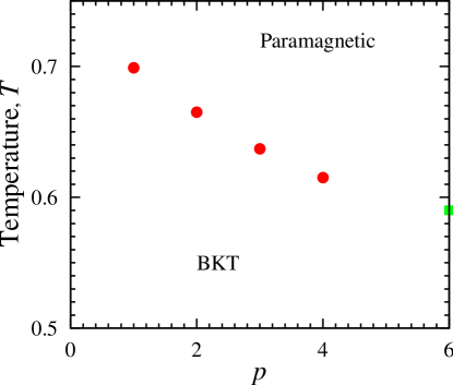
Figure 1: ($p,T$) phase diagram of the two–dimensional generalised XY model. Full circles indicate a Berezinskiǐ–Kosterlitz–Thouless like phase transition, while the square is believed to corresponds to a weak first order phase transition.

In figure 1 we show the phase diagram of the two dimensional generalised XY model in the $(p,T)$ plane. It is seen that the model exhibits a phase transition from a paramagnetic phase to a BKT–like phase as the temperature decreases. The transition temperature is evaluated using Monte Carlo simulations according to reference [20]. The value of the transition temperature corresponding to $p=1$ is taken from reference [21].

2.2 Three dimensions

For $d=3$, different analytical approximations, such as a Mean Field (MF) approach, as well as its Two–Site Cluster (TSC) refinement have been used in reference [18] to estimate transition temperatures for $p=2,3,4$, and then for higher values of $p$ in subsequent papers (see below). Notice also that $(\sin\theta)^{p}$, and hence the absolute value of the interaction potential, decreases with increasing $p$, and this aspect is reflected by the $p$–dependence of the estimated transition temperature. Transition temperatures have been estimated in reference [22] by self–consistent harmonic approximation, both for $d=2$ and $d=3$, and it was found that the transition temperature is decreasing against $p$. A study of the model in its continuum limit, carried out in reference [22] also showed that out–of–plane fluctuations, and consequently the magnon density, decrease with increasing $p$.

We have also addressed the three dimensional generalised XY models for various values of $p$, by means of Monte Carlo (MC) simulation. We have investigated the transitional behaviour of various thermodynamic functions, such as the susceptibility and the specific heat, and made comparisons with MF and TSC predictions. MF yielded a tricritical behaviour with tricritical points having real (non–integer) values of the parameter $p$. As for simulation results, transitional behaviour characetristic of the XY model was found for $p=2,3,4,8$, the case $p=12$ suggested tricritical behaviour, whereas evidence of first–order transitions was obtained for $p=16,20$.

In Figure 2 we present the $(p,T)$ phase diagram, where we can read off the behaviour of the transition temperature as a function of $p$ for $1\leq p\leq 20$. MF and TSC data can be found in references [18, 23, 24, 19], while Monte carlo data are taken from references [25, 23, 24]. Notice that, for $p\leq 4$, TSC gives better estimates of $T_{c}$ than MF, then the two roles are exchanged for $p=8,12$, and finally the three methods give very similar answers when $p\geq 16$, i.e. where the transition has a pronounced first–order character.

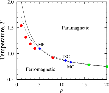
Figure 2: Phase diagram of the three dimensional generalised XY model. The solid and dashed lines stand for transition temperatures estimated via mean–field and two–site–cluster treatments, respectively. Full circles and squares indicate second and first order phase transitions temperatures evaluated via Monte Carlo simulations, respectively. Full diamonds shows the locations of tricritical points.

3 Annealed dilution in ferromagnets

Another class of systems that has been extensively studied in the literature spans those with random impurities (disorder). For a review on diluted magnetism see reference [26]. The interest in these systems stems from the fact that in nature no system is really pure. Indeed, the presence of cavities, grain boundaries, lattice defects, chemical impurities (i.e. of other chemical individuals) or some other kind of disorder may affect the properties of the pure system, and result in different effects. To consider a simple but rather important example, in a system of magnetically coupled spins, some lattice sites may be occupied by nonmagnetic constituents (site–dilution). Both in experimental and theoretical terms, one can distinguish between annealed and quenched disorder.

In quenched systems, impurities are held frozen in randomly distributed fixed positions, without the possibility of overcoming potential barriers for diffusing into the host material: in this case the relaxation time is very long and thermal equilibrium between impurities and the constituents of the host is never reached. In annealed materials, impurities are allowed to diffuse randomly and to reach thermal equilibrium with the other constituents of the host material. One can also think of a two–component solution being very dilute with respect to one of the components. When the system is in the liquid phase, molecules of the two types can exchange their positions, and diffuse throughout the sample. Let then the system crystallize, at sufficiently low temperature. In the resulting solid, particles of the minority component are fixed in certain lattice sites only.

The simplest extension of equation (5) taking these situations into account reads

$$\mathscr{H}_{\mathrm{dis.}}=-\frac{J}{2}\sum_{\langle i,j\rangle}\nu_{i}\nu_{j}\ \bm{s}_{i}\cdot\bm{s}_{j}.$$ (9)

where the occupation numbers $\nu_{i}$ equal “zero” for a site $i$ hosting a nonmagnetic impurity and “one” for a magnetic particle. The density of magnetic particles in the system is defined via

$$\rho=\frac{1}{N}\sum_{i}^{N}\langle\nu_{i}\rangle.$$

Within this notation the pure system, i.e. without impurities, corresponds to $\rho=1$.

In the annealed case, Hamiltonian (9) can be interpreted as describing a two–component system consisting of interconverting “real” ($\nu_{i}=1$) and “ghost”, “virtual” or ideal–gas particles ($\nu_{i}=0$). Both kinds of particles have the same kinetic energy, and the total number of particles equals the number of available lattice sites. In this case one works in the Grand–Canonical Ensemble where the probability (1) for a configuration, now involving the occupation numbers $\{\nu_{i}\}$, as well as the spins $\{\bm{s}_{i}\}$, is defined by

$$\mathscr{P}\propto\exp\left[-\beta\left(\mathscr{H}_{\mathrm{dis.}}-\mu\sum_{i}\nu_{i}\right)\right],$$ (10)

where $\mu$ denotes the excess chemical potential of “real” particles over “ideal” ones. Of course, the interaction may be anisotropic in spin space, as in the cases outlined above, or involve more distant neighbours. The system remains translationally invariant on average. This model bears some similarity with the Blume–Emery–Griffiths model [27] for ³He impurities in superfluid ⁴He. More precisely, notice also that, starting from an assigned model, its lattice gas extensions can be written in general as

$$\mathscr{H}_{LG}=-\frac{J}{2}\sum_{\langle i,j\rangle}\nu_{i}\nu_{j}\ \bm{s}_{i}\cdot\bm{s}_{j}+\frac{\lambda}{2}\sum_{\langle i,j\rangle}\nu_{i}\nu_{j}\ ,$$ (11)

where the purely positional $\lambda$ term only becomes immaterial in the pure limit $\mu\rightarrow+\infty$. In equation (9) we have chosen the simplest case $\lambda=0$. Lattice gas models can be used to model adsorption, and, in general, the variable occupation numbers produce some fluidity of the system. One can also set the coupling $J$ term to zero, so that the resulting model becomes isomorph with an Ising model in external field. In general, the interplay between $J$ and $\lambda$ can produce a richer phase diagram: for example, when $\lambda>0$ and $\mu$ is sufficiently large, the ground state may exhibit checkerboard positional order but no orientational one.

It is very well known that a small amount of annealed disorder does not affect the way the singularities take place in pure systems i.e. the phase transition remains a second order one. The $\rho$–dependent critical temperature is shifted towards $T_{c}(\rho)<T_{c}(1)$. If the chemical potential $\mu$ is held fixed, the properties of the phase transition are the same as those known for the pure system, corresponding to $\mu\to\infty$ and $\rho=1$. If, however, the concentration $\rho$ is kept fixed during the transition, care must taken in characterising the transition. For details see reference [28].

A significant amount of impurities may alter the order of the phase transition or make it disappear. Investigations of the XY model, as a protype for He³ – He⁴ mixtures, in three dimensions, via high temperature series expansion of the partition function, show that by increasing the density of randomness the transition temperature decreases. At a certain value of $\rho$ the transition changes its nature and turns into a first order one [29]. The second order phase transition line ends at a tricritical point, which marks the begining of a line of fisrt–oder phase transition temperature that keeps decreasing as the concentration of impurities increases.

In the three–dimensional case, the topology of the phase diagram of model (9) had been investigated by MF and TSC approximations for the Ising [30], as well as PR cases [31] in the presence of a magnetic field, and for He at zero magnetic field [32]. These investigations were later extended [33] to the extremely anisotropic (Ising–like) two–dimensional model, and in the absence of a magnetic field, as well. The studied models were found to exhibit a tricritical behaviour i.e. the ordering transition turned out to be of first order for $\mu$ below an appropriate threshold, and of second order above it. When the transition is of first order, the orientationally ordered phase is also denser than the disordered one.

To check the predictions of the molecular–field–like treatments used to construct the phase diagrams, extensive Monte Carlo simulations has been performed [31, 32, 33] for particular values of the chemical potential. A number of thermodynamic and structural properties had been investigated. It had been found that there is a second order ferromagnetic phase transition manifested by a significant growth of magnetic and density fluctuations. The transition temperatures were found to be smaller than those of the corresponding values for the pure systems and the critical behaviour of the investigated models to be consistent with that of their pure counterparts. Furthermore it had been found that MF yields a qualitatively correct picture, and the quantitative agreement with simulation could be improved by TSC, which has the advantage of predicting two–site correlations. In general we found that simulations results are consistent with the molecular–field like treatments.

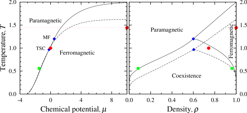
Figure 3: Phase diagrams of the three–dimensional Heisenberg model in the chemical potential – temperature and density – temperature planes. Solid and dashed lines correspond to mean–field and two–site–cluster results, respectively. Circles and squares stand, respectively, for estimates of the second and first order transition temperatures using Monte Carlo simulations. Diamonds mark the locations of tricritical points. The dotted line marks the transition temperature of the model in the absence of impurities.

In figure 3 we report the phase diagrams in the chemical potential – temperature and density – temperature planes. We show the behaviour of the transition temperature $T_{c}$ versus chemical potential $\mu$. The plot also shows a fast, approximately linear, increase of $T_{c}$ with $\mu$ up to $\mu\approx 0$, and a slower one above this value. Moreover, MF and TSC results essentially coincide up to $\mu\approx 0$. In the phase diagram in the ($\rho,T$) plane the existence of a first–order transition is reflected by a biphasic region. We found that the system exhibits a first–order phase transition from a dense BKT phase to a paramagnetic one. In the temperature–density phase diagram, both phases are expected to coexist over some range of densities and temperatures.

Two–dimensional annealed lattice models were investigated [34, 35] as well, and the obtained results for $\mu=0$ or a moderately negative $\mu$ were found to support a BKT phase transition with a transition temperature lower than that of the pure parent due to the presence of impurities. For negative and sufficiently large in magnitude $\mu$ we found evidence of a first order phase transition in agreement with renormalization group treatments [36, 37].

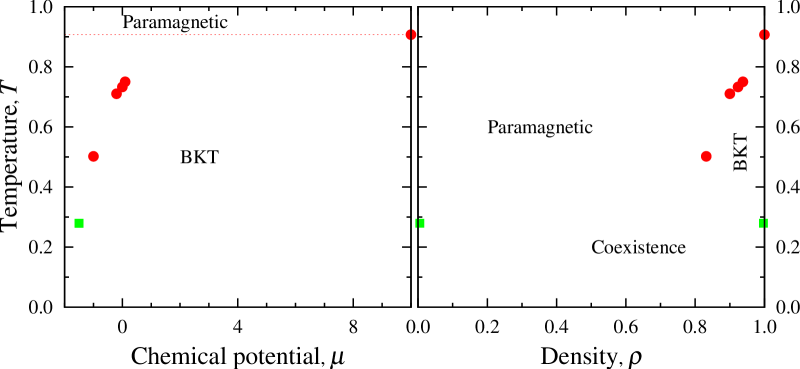
Figure 4: Phase diagrams of the two–dimensional planar rotator. Circles and squares stand, respectively, for estimates of the second and first order transition temperatures using Monte Carlo simulations. Diamonds mark the locations of tricritical points. The dotted line marks the transition temperature of the model in the absence of impurities.

In figure 4 we show the phase diagram in the $(\rho,T)$ plane. The existence of a first–order transition is reflected here by a biphasic (binodal) region. The phase diagram obtained here is similar to the one resulting from the study of the diluted planar rotator model [31].

So far, we have discussed isotropic models. As we have mentioned, in addition to dilution one can consider anisotropic interactions as well. In reference [33] we have investigated two–dimensional continuous Ising spin models with two and tree component spins. The phase diagrams of these models were found to be topologically similar to those found for the Heisenberg model shown in figure 3. The main differences come from the locations of the phase boundaries.

4 Conclusion

The Statistical Mechanics of lattice systems is essentially based on the study of a number of relatively “simple” models which are gradually made more complicated. We have shown here some examples, involving generalized XY models and annealed magnetic systems, where rigorous results have been produced to prove existence and type of transition, supplemented by a variety of techniques (MF or TSC approximation and Monte Carlo simulation) for elucidating the resulting physical behaviour and estimating numerical values.

We obtained the phase diagram in two and three dimensions of a generalized version of the lattice XY model, where the out–of–plane fluctuations of the spins are controlled by a parameter $p$. Our investigation shows that the nature of the transition is highly affected by the strength of the out–of–plane fluctuations. For $p\geq 12$ at three dimensions and $p\gtrsim 6$ at two dimensions, it is first order, whereas for small values its transitional behaviour coincides with that of the original XY model. The transition temperature is found to decrease as $p$ increases at any dimension.

We constructed the phase diagrams of the annealed lattice plane rotator in two dimensions and the Heisenberg model in three dimensions. It is found that the transition changes from a second order at three dimensions and Berezinskiǐ–Kosterlitz–Thouless at two dimensions into a first order transition as the concentration of impurities is increased. In turn the transition temperature is found to decrease with increasing impurity density.

This work was supported by the Ministry of Education and Science of Bulgaria under Grant No $\Phi$–1517.

References

- [1] Yeomans J M 1992 Statistical Mechanics of Phase Transitions (New York: Oxford University Press)
- [2] Pathria R K 1996 Statistical mechanics 2nd ed (Oxford, England: Butterworth–Heinemmann)
- [3] Mazenko G F 2003 Fluctuations, Order and Defects (Hoboken: Wiley)
- [4] Berezinskiǐ V L 1971 Sov. Phys. JETP 32 493–500 [Zh. Eksp. Teor. Fiz. 59, 907–920]
- [5] Kosterlitz J M and Thouless D J 1973 J. Phys. C: Solid State Phys. 6 1181–1203
- [6] Stanley H E 1968 Phys. Rev. 176 718–722
- [7] Berlin T H and Kac M 1952 Phys. Rev. 86 821–835
- [8] Georgii H O 1988 Gibbs Measures and Phase Transitions (de Gruyter Studies in Mathematics vol 9) (Berlin: Walter de Gruyter)
- [9] Sinai Y G 1982 Theory of Phase Transitions: Rigorous Results (Oxford: Pergamon)
- [10] Pelissetto A and Vicari E 2002 Phys. Rep. 368 549–727
- [11] Mermin N D and Wagner H 1966 Phys. Rev. Lett. 17 1133–1136
- [12] Gulácsi Z and Gulácsi M 1998 Adv. Phys. 47 1–89
- [13] Fisher M E 1998 Rev. Mod. Phys. 70 653–681
- [14] Stanley H E 1999 Rev. Mod. Phys. 71 S358–S366
- [15] de Jongh L J and Miedema A R 2001 Adv. Phys. 50 947–1170
- [16] Binder K 1987 Rep. Prog. Phys. 50 783–859
- [17] Cardy J 1996 Scaling and Renormalization in Statistical Physics (Cambridge Lecture Notes in Physics vol 5) (Cambridge, England: Cambridge University Press)
- [18] Romano S and Zagrebnov V 2002 Phys. Lett. A 301 402–407
- [19] van Enter A C D, Romano S and Zagrebnov V A 2006 J. Phys. A: Math. Gen. 39 L439–L445
- [20] Mól L, Pereira A R, Chamati H and Romano S 2006 Eur. Phys. J. B 50 541–548
- [21] Evertz H G and Landau D P 1996 Phys. Rev. B 54 12302–12317
- [22] Mól L A S, Pereira A R and Moura-Melo W A 2003 Phys. Lett. A 319 114–121
- [23] Chamati H, Romano S, Mól L and Pereira A R 2005 Eur. Phys. Lett. 72 62–68
- [24] Chamati H and Romano S 2006 Eur. Phys. J B 54 249–254
- [25] Costa B V, Pereira A R and Pires A S T 1996 Phys. Rev. B 54 3019–3021
- [26] Stinchcombe R B 1983 Dilute Magnetism Phase Transitions and Critical Phenomena vol 7 ed Domb C and Lebowitz J L (London: Academic Press) chap 3, pp 151–280
- [27] Blume M, Emery V J and Griffiths R B 1971 Phys. Rev. A 4 1071–1077
- [28] Fisher M E 1968 Phys. Rev. 176 257–272
- [29] Reeve J S 1976 J. Phys. C: Solid State Phys. 9 2575–2587
- [30] Sokolovskii R O 2000 Phys. Rev. B 61 36–39
- [31] Romano S and Sokolovskii R O 2000 Phys. Rev. B 61 11379–11390
- [32] Chamati H and Romano S 2005 Phys. Rev. B 72 064424
- [33] Chamati H and Romano S 2005 Phys. Rev. B 72 064444
- [34] Chamati H and Romano S 2006 Phys. Rev. B 73 184424
- [35] Chamati H and Romano S 2007 Phys. Rev. B 75 184413
- [36] Cardy J L and Scalapino D J 1979 Phys. Rev. B 19 1428–1436
- [37] Berker A N and Nelson D R 1979 Phys. Rev. B 19 2488–2503