Supersymmetry non-renormalization theorem from a computer and the AdS/CFT correspondence

Abstract:

We perform Monte Carlo calculation of correlation functions in 4d $\mathcal{N}=4$ super Yang-Mills theory on $R\times S^{3}$ in the planar limit. In order to circumvent the well-known problem of lattice SUSY, we adopt the idea of a novel large-$N$ reduction, which reduces the calculation to that of corresponding correlation functions in the plane-wave matrix model or the BMN matrix model. This model is a 1d gauge theory with 16 supersymmetries, which can be simulated in a manner similar to the recent studies of the D0-brane system. We study two-point and three-point functions of chiral primary operators at various coupling constant, and find that they agree with the free theory results up to overall constant factors. The ratio of the overall factors for two-point and three-point functions agrees with the prediction of the AdS/CFT correspondence.

1 Introduction

The gauge-gravity duality [1] has been one of the most important subjects in string theory over the past decade. The most typical example is the so-called AdS/CFT correspondence between type IIB superstring theory on $AdS_{5}\times S^{5}$ and 4d ${\cal N}=4$ U($N$) super Yang-Mills theory (SYM). Even in this case, however, a complete proof of the duality is still missing. In particular, the region described by the classical supergravity on the string theory side corresponds to the strongly coupled region in the planar large-$N$ limit on the SYM side. In order to study the strongly coupled 4d ${\cal N}=4$ SYM from first principles, one needs to have a non-perturbative formulation such as the lattice QCD. The problem here is that the lattice regularization necessarily breaks translational symmetry, which is included in the supersymmetry (SUSY). In order to restore SUSY in the continuum limit, one generally has to fine-tune parameters in the lattice action. In fact any lattice formulations of 4d ${\cal N}=4$ SYM proposed so far seem to require fine-tuning of at least three parameters [2].

Since 4d ${\cal N}=4$ SYM has conformal symmetry, the theory on $R^{4}$ is equivalent to the theory on $R\times S^{3}$ through conformal mapping. The novel large-$N$ reduction [3] connects the planar large-$N$ limit of this theory to a reduced model, which can be obtained by shrinking the $S^{3}$ to a point. The resulting one-dimensional gauge theory with 16 supercharges can be studied by using the Fourier-mode simulation [4] as in recent studies of the D0-brane system [5]. Thus we can perform Monte Carlo calculations in 4d ${\cal N}=4$ SYM respecting SUSY maximally and without fine-tuning.

In this article we present explicit results for correlation functions of chiral primary operators (CPOs) in 4d $\mathcal{N}=4$ SYM. In particular, we find that the two-point and three-point functions agree with the free theory results up to overall constant factors even at fairly strong coupling. Moreover the ratio of the overall factors agrees with the prediction of the AdS/CFT correspondence.

2 Large-$N$ reduction for ${\cal N}=4$ SYM on $R\times S^{3}$

Let us first discuss the novel large-$N$ reduction for ${\cal N}=4$ SYM on $R\times S^{3}$. By collapsing the $S^{3}$ to a point, we obtain the plane wave matrix model (PWMM) or the BMN matrix model [9], whose action is given by

$$S_{\rm PW} = \frac{1}{g_{\rm PW}^{2}}\int dt\,{\rm tr\,}\left[\frac{1}{2}(D_{t}X_{M})^{2}-\frac{1}{4}[X_{M},X_{N}]^{2}+\frac{1}{2}\Psi^{\dagger}D_{t}\Psi-\frac{1}{2}\Psi^{\dagger}\gamma_{M}[X_{M},\Psi]\right.$$ (1)

$$\quad\quad\left.+\frac{\mu^{2}}{2}(X_{i})^{2}+\frac{\mu^{2}}{8}(X_{a})^{2}+i\mu\epsilon_{ijk}X_{i}X_{j}X_{k}+i\frac{3\mu}{8}\Psi^{\dagger}\gamma_{123}\Psi\right]\ .$$

Here the parameter $\mu$ is related to the radius of $S^{3}$ as $R_{S^{3}}=\frac{2}{\mu}$, and the covariant derivative is defined by $D_{t}=\partial_{t}-i[A,\ \cdot\ ]$, where $A(t)$, as well as $X_{M}(t)$ and $\Psi(t)$, is an $N\times N$ hermitian matrix. The range of indices is given by $1\leq M,N\leq 9$, $1\leq i,j,k\leq 3$ and $4\leq a\leq 9$. The model has the SU$(2|4)$ symmetry with 16 supercharges.

In fact the model possesses many discrete vacua representing multi fuzzy spheres, which are given explicitly by

$$X_{i}=\mu\bigoplus_{I=1}^{\nu}\Bigl{(}L_{i}^{(n_{I})}\otimes{\bf 1}_{k_{I}}\Bigr{)}\ \quad\mbox{with}\ \ \sum_{I=1}^{\nu}n_{I}k_{I}=N\ ,$$ (2)

where $L_{i}^{(r)}$ are the $r$-dimensional irreducible representation of the SU$(2)$ algebra $[L_{i}^{(r)},L_{j}^{(r)}]=i\,\epsilon_{ijk}\,L_{k}^{(r)}$. These vacua preserve the SU$(2|4)$ symmetry, and are all degenerate.

In order to retrieve the planar ${\cal N}=4$ SYM on $R\times S^{3}$, one has to pick up a particular background from (2), and consider the theory (1) around it. Let us consider the case

$$k_{I}=k\ ,\quad n_{I}=n+I-\frac{\nu+1}{2}\quad\quad\mbox{for\ \ $I=1,\cdots,\nu$}\ ,$$ (3)

and take the large-$N$ limit in such a way that

$$k\rightarrow\infty\ ,\ \frac{n}{\nu}\rightarrow\infty\ ,\ \nu\rightarrow\infty\ ,\quad\mbox{with}\;\;\lambda_{\rm PW}\equiv\frac{g_{\rm PW}^{2}k}{n}\;\;\mbox{fixed}\ .$$ (4)

Then the resulting theory is claimed [3] to be equivalent to the planar limit of ${\cal N}=4$ SYM on $R\times S^{3}$ with the ’t Hooft coupling constant given by

$$\lambda_{\rm SYM}=2\pi^{2}\lambda_{\rm PW}(R_{S^{3}})^{3}=\frac{16\pi^{2}k}{n}\frac{g_{\rm PW}^{2}}{\mu^{3}}\ .$$ (5)

The above equivalence may be viewed as an extension of the large-$N$ reduction [15], which asserts that the large-$N$ gauge theories can be studied by dimensionally reduced models. The original idea for theories compactified on a torus can fail due to the instability of the U(1)^D symmetric vacuum of the reduced model [16]. This problem is avoided in the novel proposal since the PWMM is a massive theory and the vacuum preserves the maximal SUSY. Since the planar limit is taken in the reduced model, the instanton transition to other vacua and the “fuzziness” of the spheres are suppressed. Viewed as a regularization of the ${\cal N}=4$ SYM on $R\times S^{3}$, the present formulation respects the maximal ${\rm SU}(2|4)$ symmetry (with 16 supercharges) of the PWMM, and in the limit (4) the symmetry is expected to enhance to the full superconformal ${\rm SU}(2,2|4)$ symmetry (with 32 supercharges). Since any kind of UV regularization breaks the conformal symmetry, this regularization is optimal from the viewpoint of preserving SUSY.

3 Correlation functions in 4d $\mathcal{N}=4$ SYM

As simple examples of $1/2$ BPS operators, let us consider the CPOs given by

$$\mathcal{O}^{R^{4}}_{\Delta}(x)=T_{a_{1}\cdots a_{\Delta}}\ {\rm tr\,}\left(X^{R^{4}}_{a_{1}}X^{R^{4}}_{a_{2}}\cdots X^{R^{4}}_{a_{\Delta}}(x)\right)\ ,$$ (6)

where $T_{a_{1}\cdots a_{\Delta}}$ is a symmetric traceless tensor and $X_{a}^{R^{4}}$ represents the six scalars in 4d $\mathcal{N}=4$ SYM on $R^{4}$. Thanks to the conformal symmetry, the forms of two-point and three-point functions of the CPOs are determined as

$$\left\langle\mathcal{O}^{R^{4}}_{\Delta}(x_{1})\mathcal{O}^{R^{4}}_{\Delta}(x_{2})\right\rangle = c_{\Delta}\left\langle\mathcal{O}^{R^{4}}_{\Delta}(x_{1})\mathcal{O}^{R^{4}}_{\Delta}(x_{2})\right\rangle_{\rm free}\ ,$$

$$\left\langle\mathcal{O}^{R^{4}}_{\Delta_{1}}(x_{1})\mathcal{O}^{R^{4}}_{\Delta_{2}}(x_{2})\mathcal{O}^{R^{4}}_{\Delta_{3}}(x_{3})\right\rangle = c_{\Delta_{1}\Delta_{2}\Delta_{3}}\left\langle\mathcal{O}^{R^{4}}_{\Delta_{1}}(x_{1})\mathcal{O}^{R^{4}}_{\Delta_{2}}(x_{2})\mathcal{O}^{R^{4}}_{\Delta_{3}}(x_{3})\right\rangle_{\rm free}\ ,$$ (7)

where $c_{\Delta}$ and $c_{\Delta_{1}\Delta_{2}\Delta_{3}}$ are over-all constants depending on $\lambda_{\rm SYM}$ in general, and $\langle\cdots\rangle_{\rm free}$ denotes the results of free theory. The analysis on the gravity side suggests [17]

$$\left.\frac{c_{\Delta_{1}\Delta_{2}\Delta_{3}}}{\sqrt{c_{\Delta_{1}}c_{\Delta_{2}}c_{\Delta_{3}}}}\right|_{N\rightarrow\infty,\lambda_{\rm SYM}\rightarrow\infty}=\left.\frac{c_{\Delta_{1}\Delta_{2}\Delta_{3}}}{\sqrt{c_{\Delta_{1}}c_{\Delta_{2}}c_{\Delta_{3}}}}\right|_{N\rightarrow\infty,\lambda_{\rm SYM}\rightarrow 0}=1\quad\mbox{for}\ \ ^{\forall}\Delta_{i}\ .$$ (8)

In order to relate the above operators to those in the PWMM, we first perform the conformal mapping from $R^{4}$ to $R\times S^{3}$. Then the $M$-point functions of the CPO $\mathcal{O}^{R\times S^{3}}_{\Delta_{i}}$ on $R\times S^{3}$ are related to those in PWMM as

$$\int\frac{d\Omega_{3}^{(1)}}{2\pi^{2}}\cdots\int\frac{d\Omega_{3}^{(M)}}{2\pi^{2}}\left\langle\mathcal{O}_{\Delta_{1}}^{R\times S^{3}}(t_{1},\Omega_{3}^{(1)})\cdots\mathcal{O}_{\Delta_{M}}^{R\times S^{3}}(t_{M},\Omega_{3}^{(M)})\right\rangle=\frac{1}{n^{M}\nu}\left\langle\mathcal{O}_{\Delta_{1}}^{\rm PW}(t_{1})\cdots\mathcal{O}_{\Delta_{M}}^{\rm PW}(t_{M})\right\rangle\ ,$$ (9)

where we have defined $\mathcal{O}^{\rm PW}_{\Delta}(t)=T_{a_{1}\cdots a_{\Delta}}\ {\rm tr\,}\Big{(}X_{a_{1}}X_{a_{2}}\cdots X_{a_{\Delta}}(t)\Big{)}$ [3].

We calculate the two-point functions $\Big{\langle}{\rm tr\,}Z^{2}(t_{1})\,{\rm tr\,}Z^{{\dagger}2}(t_{2})\Big{\rangle}$, where $Z=\frac{1}{\sqrt{2}}(X_{4}+iX_{5})$, and the three-point functions $\Big{\langle}{\rm tr\,}\Big{(}X_{4}X_{5}(t_{1})\Big{)}\,{\rm tr\,}\Big{(}X_{5}X_{6}(t_{2})\Big{)}\,{\rm tr\,}\Big{(}X_{6}X_{4}(t_{3})\Big{)}\Big{\rangle}$. The CPOs we consider here have $\Delta=2$, and the AdS/CFT predicts $c_{222}=c_{2}^{3/2}$, which we test by Monte Carlo calculations.

4 Monte Carlo method

In order to simulate the PWMM (1), we compactify the $t$-direction to a circle of circumference $\beta$. Since we are interested in the properties at zero temperature, we impose periodic boundary conditions on both scalars $X_{i}(t)$ and fermions $\Psi_{\alpha}(t)$, which keep SUSY intact. In Fourier-mode simulation [4], we first fix the gauge symmetry completely by choosing $A(t)=\frac{1}{\beta}{\rm diag}(\alpha_{1},\cdots,\alpha_{N})$ with $-\pi<\alpha_{a}\leq\pi$, and then make a Fourier expansion  $X_{i}(t)=\sum_{n=-\Lambda}^{\Lambda}\tilde{X}_{i,n}e^{i\omega nt}\ (\omega\equiv\frac{2\pi}{\beta})$ and similarly for the fermions. The upper bound $\Lambda$ on the Fourier modes plays the role of the UV cutoff. The original PWMM can be retrieved by just taking the limits $\beta\rightarrow\infty$ and $\frac{\Lambda}{\beta}\rightarrow\infty$ since there are neither UV nor IR divergences. The model regularized by finite $\beta$ and $\Lambda$ can be simulated by the RHMC algorithm. This method has been applied extensively to the D0-brane system corresponding to $\mu=0$, and the results confirmed the gauge/gravity duality for various observables [5].

Since the parameter $g_{\rm PW}^{2}$ in the action (1) can be scaled away by appropriate redefinition of fields and parameters, we take $g_{\rm PW}^{2}N=1$ without loss of generality as in refs. [5]. In this convention one finds from eq. (5) that the small (large) $\mu$ region in the PWMM corresponds to the strong (weak) coupling region in the 4d $\mathcal{N}=4$ SYM.

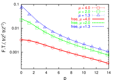
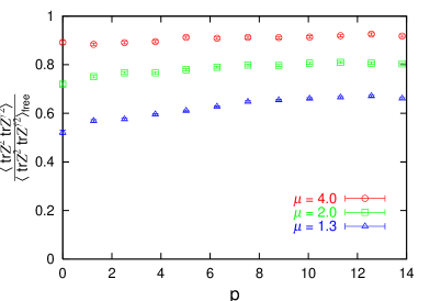
Figure 1: (Left) The two-point function $\Big{\langle}{\rm tr\,}\widetilde{Z^{2}}(p)\ {\rm tr\,}\widetilde{Z^{{\dagger}2}}(-p)\Big{\rangle}$ is plotted in the log scale. The curves represent the corresponding free theory results multiplied by 0.919, 0.799, 0.647 for $\mu=4.0,2.0,1.3$, respectively. (Right) The ratio of the two-point function to the corresponding free theory result is plotted in the linear scale for $\mu=4.0,2.0,1.3$.

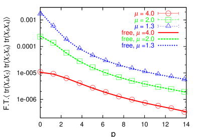
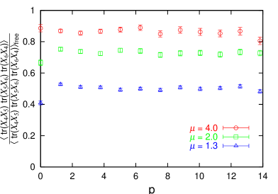
Figure 2: (Left) The three-point function $\Big{\langle}{\rm tr\,}\left(\widetilde{{X}_{4}X_{5}}(p)\right)\,{\rm tr\,}\left(\widetilde{X_{5}X_{6}}(0)\right)\,{\rm tr\,}\left(\widetilde{X_{6}X_{4}}(-p)\right)\Big{\rangle}$ is plotted in the log scale. The curves represent the corresponding free theory results multiplied by 0.850, 0.716, 0.491 for $\mu=4.0,2.0,1.3$, respectively. (Right) The ratio of the three-point function to the corresponding free theory result is plotted in the linear scale for $\mu=4.0,2.0,1.3$.

5 Numerical results

The parameters describing the background (3) are chosen as $n=\frac{3}{2},\nu=2,k=2$, which corresponds to the matrix size $N=6$. We use (2) with (3) as the initial configuration and check that no transition to other vacua occurs during the simulation. The values of $\mu$ we use are $\mu=4.0,2.0,1.3$, which correspond to $\lambda_{\rm SYM}\simeq 0.55,4.39,16.0$, respectively, in the chosen background. Thus we cover a wide range of the coupling constant. The regularization parameters in the $t$-direction are taken as $\beta=5.0,\Lambda=12$ for all cases.

In fig. 1 (Left) we plot the two-point function $\Big{\langle}{\rm tr\,}\widetilde{Z^{2}}(p)\,{\rm tr\,}\widetilde{Z^{{\dagger}2}}(-p)\Big{\rangle}$. We find that the results agree well — up to overall constants depending on $\mu$ — with the corresponding free theory results, which are obtained by just switching off the interaction terms in the reduced model with the same regularization parameters. In fig. 1 (Right) we plot the ratio to the free theory results. Figure 2 shows similar results for the three-point function $\Big{\langle}{\rm tr\,}\left(\widetilde{{X}_{4}X_{5}}(p)\right)\,{\rm tr\,}\left(\widetilde{X_{5}X_{6}}(0)\right)\,{\rm tr\,}\left(\widetilde{X_{6}X_{4}}(-p)\right)\Big{\rangle}$.

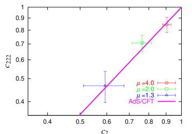
Figure 3: The overall constants corresponding to $c_{2}$ and $c_{222}$ in eq. (7) are plotted in the log-log scale. The straight line presents the relation $c_{222}=c_{2}^{3/2}$ predicted by the AdS/CFT.

We can extract the the overall constants corresponding to $c_{2}$ and $c_{222}$ in eq. (7) from figs. 1 and 2, respectively. Since the data on the right panels are not completely constant in $p$, we take the maximum and minimum values as the upper and lower bounds of the estimates. In fig. 3 we plot the overall constants obtained in this way for three values of $\mu$. The data points represent the mean value of the upper and lower bounds. We find that our results for various coupling constants lie on the straight line which represents the prediction $c_{222}=c_{2}^{3/2}$ from the AdS/CFT. Our results therefore suggest that the relation (8) holds also at intermediate coupling constants.

6 Summary and discussions

We have made the first attempt to investigate nonperturbative properties of the 4d $\mathcal{N}=4$ SYM from first-principle calculations. Our formulation is considered optimal in preserving SUSY, which seems to give us the virtue of making the coupling constant dependence of the CPO correlation functions restricted mostly to the overall factors. This feature of our formulation enables us to test the prediction (8) of the AdS/CFT correspondence already for quite a small matrix size. Our results suggest that the relation extends to intermediate coupling constants as well.

In fact there is strong evidence from field theoretical analysis in the 4d $\mathcal{N}=4$ SYM that the non-renormalization theorem holds for two-point and three-point correlation functions of CPOs [19, 20], which implies $c_{\Delta}=c_{\Delta_{1}\Delta_{2}\Delta_{3}}=1$. It is therefore expected that the data points in fig. 3 will approach $c_{2}=c_{222}=1$ as we take the limit (4) for fixed $\lambda_{\rm SYM}$, which needs to be checked.

The analysis of four-point functions would be more interesting [22] since there is evidence for the non-renormalization theorem only in the extremal and next-to-extremal cases [23], and in fact the AdS/CFT predicts its violation for the other general cases in the strong coupling limit [24]. We consider it very interesting that such nonperturbative issues in 4d $\mathcal{N}=4$ SYM have become accessible by computer simulations.

- [1] J. M. Maldacena, Adv. Theor. Math. Phys. 2 (1998) 231.
- [2] See, for instance, J. Giedt, Int. J. Mod. Phys. A 24 (2009) 4045.
- [3] T. Ishii, G. Ishiki, S. Shimasaki and A. Tsuchiya, Phys. Rev. D 78 (2008) 106001.
- [4] M. Hanada, J. Nishimura and S. Takeuchi, Phys. Rev. Lett. 99 (2007) 161602.
- [5] K. N. Anagnostopoulos, M. Hanada, J. Nishimura and S. Takeuchi, Phys. Rev. Lett. 100 (2008) 021601; M. Hanada, A. Miwa, J. Nishimura and S. Takeuchi, Phys. Rev. Lett. 102 (2009) 181602; M. Hanada, Y. Hyakutake, J. Nishimura and S. Takeuchi, Phys. Rev. Lett. 102 (2009) 191602; M. Hanada, J. Nishimura, Y. Sekino and T. Yoneya, Phys. Rev. Lett. 104 (2010) 151601.
- [6] M. Hanada, S. Matsuura and F. Sugino, arXiv:1004.5513 [hep-lat]; M. Hanada, arXiv:1009.0901 [hep-lat].
- [7] J. Nishimura, PoS LAT2009 (2009) 016.
- [8] D. Berenstein and R. Cotta, JHEP 0704 (2007) 071; D. Berenstein, R. Cotta and R. Leonardi, Phys. Rev. D 78 (2008) 025008.
- [9] D. E. Berenstein, J. M. Maldacena and H. S. Nastase, JHEP 0204 (2002) 013.
- [10] N. Kawahara, J. Nishimura and K. Yoshida, JHEP 0606 (2006) 052.
- [11] G. Ishiki, S. W. Kim, J. Nishimura and A. Tsuchiya, Phys. Rev. Lett. 102 (2009) 111601; JHEP 0909 (2009) 029; Y. Kitazawa and K. Matsumoto, Phys. Rev. D 79 (2009) 065003.
- [12] S. Catterall and G. van Anders, JHEP 1009 (2010) 088.
- [13] G. Ishiki, S. Shimasaki, Y. Takayama and A. Tsuchiya, JHEP 0611 (2006) 089; T. Ishii, G. Ishiki, S. Shimasaki and A. Tsuchiya, JHEP 0705 (2007) 014; Phys. Rev. D 77 (2008) 126015.
- [14] H. Kawai, S. Shimasaki and A. Tsuchiya, Int. J. Mod. Phys. A 25 (2010) 3389; Phys. Rev. D 81 (2010) 085019.
- [15] T. Eguchi and H. Kawai, Phys. Rev. Lett. 48 (1982) 1063.
- [16] G. Bhanot, U. M. Heller and H. Neuberger, Phys. Lett. B 113 (1982) 47.
- [17] S. Lee, S. Minwalla, M. Rangamani and N. Seiberg, Adv. Theor. Math. Phys. 2 (1998) 697.
- [18] S. Catterall and T. Wiseman, JHEP 0712 (2007) 104; Phys. Rev. D 78 (2008) 041502; JHEP 1004 (2010) 077.
- [19] E. D’Hoker, D. Z. Freedman and W. Skiba, Phys. Rev. D 59 (1999) 045008.
- [20] B. Eden, P. S. Howe and P. C. West, Phys. Lett. B 463 (1999) 19.
- [21] S. S. Gubser and I. R. Klebanov, Phys. Lett. B 413 (1997) 41; D. Anselmi, D. Z. Freedman, M. T. Grisaru and A. A. Johansen, Nucl. Phys. B 526 (1998) 543; D. Z. Freedman, S. D. Mathur, A. Matusis and L. Rastelli, Nucl. Phys. B 546 (1999) 96.
- [22] M. Honda, G. Ishiki, S. W. Kim, J. Nishimura, A. Tsuchiya, in preparation.
- [23] B. U. Eden, P. S. Howe, E. Sokatchev and P. C. West, Phys. Lett. B 494 (2000) 141.
- [24] G. Arutyunov and S. Frolov, Phys. Rev. D 62 (2000) 064016.