Post-Newtonian effects on Lagrange’s equilateral triangular solution for the three-body problem

Abstract

Continuing work initiated in earlier publications [Yamada, Asada, Phys. Rev. D 82, 104019 (2010), 83, 024040 (2011)], we investigate the post-Newtonian effects on Lagrange’s equilateral triangular solution for the three-body problem. For three finite masses, it is found that the equilateral triangular configuration satisfies the post-Newtonian equation of motion in general relativity, if and only if all three masses are equal. When a test mass is included, the equilateral configuration is possible for two cases: (1) one mass is finite and the other two are zero, or (2) two of the masses are finite and equal, and the third one is zero, namely a symmetric binary with a test mass. The angular velocity of the post-Newtonian equilateral triangular configuration is always smaller than the Newtonian one, provided that the masses and the side length are the same.

I Introduction

The three-body problem in the Newton gravity represents classical problems in astronomy and physics (e.g, Danby ; Goldstein ; Marchal ). In 1765, Euler found a collinear solution for the restricted three-body problem that assumes one of three bodies is a test mass. Soon after, his solution was extended for a general three-body problem by Lagrange, who also found an equilateral triangle solution in 1772. Now, the solutions for the restricted three-body problem are called Lagrange points $L_{1},L_{2},L_{3},L_{4}$ and $L_{5}$, which are well known and described in textbooks of classical mechanics Goldstein .

Lagrange points have recently attracted renewed interests for relativistic astrophysics, where they have discussed the gravitational radiation reaction on $L_{4}$ and $L_{5}$ analytically Asada and by numerical methods SM ; Schnittman .

As a pioneering work, Nordtvedt pointed out that the location of the triangular points is very sensitive to the ratio of the gravitational mass to the inertial one Nordtvedt . Along this course, it is interesting as a gravity experiment to discuss the three-body coupling terms at the post-Newtonian order, because some of the terms are proportional to a product of three masses as $M_{1}\times M_{2}\times M_{3}$. Such a triple product can appear only for relativistic three (or more) body systems but cannot for a relativistic compact binary nor a Newtonian three-body system.

The relativistic perihelion advance of the Mercury is detected only after much larger shifts due to Newtonian perturbations by other planets such as the Venus and Jupiter are taken into account in the astrometric data analysis. In this sense, effects by the three-body coupling are worthy to investigate. Nevertheless, most of post-Newtonian works have focused on either compact binaries because of our interest in gravitational waves astronomy or N-body equation of motion (and coordinate systems) in the weak field such as the solar system (e.g. Brumberg ). Actually, future space astrometric missions such as Gaia GAIA ; JASMINE require a general relativistic modeling of the solar system within the accuracy of a micro arc-second Klioner . Furthermore, a binary plus a third body have been discussed also for perturbations of gravitational waves induced by the third body ICTN ; Wardell ; CDHL ; GMH .

The theory of general relativity is currently the most successful gravitational theory describing the nature of space and time. Hence it is important to take account of general relativistic effects on three-body configurations. The figure-eight configuration that was found decades ago Moore ; CM has been numerically studied at the first post-Newtonian ICA and also the second post-Newtonian orders LN . According to their numerical investigations, the solution remains true with a slight change in the figure-eight shape because of relativistic effects.

On the other hand, the post-Newtonian collinear configuration has been recently obtained as a relativistic extension of Euler’s collinear one, where three bodies move around the common center of mass with the same orbital period and always line up YA2010 . It may offer a useful toy model for relativistic three-body interactions, because it is tractable by hand without numerical simulations. The uniqueness of the collinear configuration has been also proven YA2011 .

Lagrange’s equilateral triangular solution has also a practical importance, since it is stable for some cases. Lagrange’s points $L_{4}$ and $L_{5}$ for the Sun-Jupiter system are stable and indeed the Trojan asteroids are located there. Clearly it is of greater importance to investigate Lagrange’s equilateral triangular solution in the framework of general relativity. Do the post-Newtonian effects admit such a triangular solution? No one doubts whether the particular configuration is still possible at the post-Newtonian order. We shall study this issue in this paper. The main purpose of this paper is to show that the equilateral triangular configuration can satisfy the post-Newtonian equation of motion, if and only if all three finite masses are equal. Throughout this paper, we take the units of $G=c=1$.

II Newtonian Lagrange’s equilateral triangular solution

First, we consider the Newton gravity among three masses denoted as $M_{I}$ $(I=1,2,3)$. The location of each mass is written as $\mbox{\boldmath$x$}_{I}$. We choose the origin of the coordinates, so that

$$M_{1}\mbox{\boldmath$x$}_{1}+M_{2}\mbox{\boldmath$x$}_{2}+M_{3}\mbox{\boldmath$x$}_{3}=0.$$ (1)

We start by seeing whether the Newtonian equation of motion for each body can be satisfied if the configuration is an equilateral triangle. Let us put $R_{12}=R_{23}=R_{31}\equiv a$, where we define the relative position between masses as

$$\mbox{\boldmath$R$}_{IJ}\equiv\mbox{\boldmath$x$}_{I}-\mbox{\boldmath$x$}_{J},$$ (2)

and $R_{IJ}\equiv|\mbox{\boldmath$R$}_{IJ}|$ for $I,J=1,2,3$. Then, the equation of motion for each mass becomes

$$\frac{d^{2}\mbox{\boldmath$x$}_{I}}{dt^{2}}=-M\frac{\mbox{\boldmath$x$}_{I}}{a^{3}},$$ (3)

where $M$ denotes the total mass $\sum_{I}M_{I}$. Therefore, it is possible that each body moves around the common center of mass with the same orbital period. Eq. (3) gives

$$\omega_{N}^{2}=\frac{M}{a^{3}},$$ (4)

where $\omega_{N}$ denotes the Newtonian angular velocity.

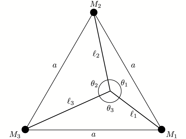
Figure 1: Equilateral triangular configuration. Each mass is located at one of the apices. We define $\theta_{I}$ ($I=1,2,3$) with respect to the common center of mass.

Figure 1 shows an equilateral triangular configuration. Let $\mbox{\boldmath$\ell$}_{I}$ denote the relative position vector of each mass with respect to the common center of mass (but not the geometrical center of the triangle) in the corotating frame with the angular velocity $\omega_{N}$. The angles between $(\mbox{\boldmath$\ell$}_{2},\mbox{\boldmath$\ell$}_{1})$, $(\mbox{\boldmath$\ell$}_{3},\mbox{\boldmath$\ell$}_{2})$ and $(\mbox{\boldmath$\ell$}_{1},\mbox{\boldmath$\ell$}_{3})$ are defined cyclically as $\theta_{1}$, $\theta_{2}$ and $\theta_{3}$ respectively. They are constant with time. There is an identity as $\theta_{1}+\theta_{2}+\theta_{3}=2\pi$, which can be used to delete one of the angles. The orbital radius $\ell_{I}\equiv|\mbox{\boldmath$\ell$}_{I}|$ of each body with respect to the common center of mass is obtained as Danby

$$\ell_{1} = \frac{a}{M}\sqrt{M_{2}^{2}+M_{2}M_{3}+M_{3}^{2}},$$ (5)

$$\ell_{2} = \frac{a}{M}\sqrt{M_{1}^{2}+M_{1}M_{3}+M_{3}^{2}},$$ (6)

$$\ell_{3} = \frac{a}{M}\sqrt{M_{1}^{2}+M_{1}M_{2}+M_{2}^{2}}.$$ (7)

III Post-Newtonian equilateral triangular solution

Next, we consider the post-Newtonian effects on the triangular configuration by employing the Einstein-Infeld-Hoffman (EIH) equation of motion as MTW ; LL ; AFH

$$\frac{d\mbox{\boldmath$v$}_{K}}{dt} = \sum_{A\neq K}\mbox{\boldmath$R$}_{AK}\frac{M_{A}}{R_{AK}^{3}}\left[1-4\sum_{B\neq K}\frac{M_{B}}{R_{BK}}-\sum_{C\neq A}\frac{M_{C}}{R_{CA}}\left(1-\frac{\mbox{\boldmath$R$}_{AK}\cdot\mbox{\boldmath$R$}_{CA}}{2R_{CA}^{2}}\right)\right.$$ (8)

$$\left.~{}~{}~{}~{}~{}~{}~{}~{}~{}~{}~{}~{}~{}~{}~{}~{}~{}~{}~{}~{}~{}+v_{K}^{2}+2v_{A}^{2}-4\mbox{\boldmath$v$}_{A}\cdot\mbox{\boldmath$v$}_{K}-\frac{3}{2}\left(\mbox{\boldmath$v$}_{A}\cdot\mbox{\boldmath$n$}_{AK}\right)^{2}\right]$$

$$-\sum_{A\neq K}(\mbox{\boldmath$v$}_{A}-\mbox{\boldmath$v$}_{K})\frac{M_{A}\mbox{\boldmath$n$}_{AK}\cdot(3\mbox{\boldmath$v$}_{A}-4\mbox{\boldmath$v$}_{K})}{R_{AK}^{2}}$$

$$+\frac{7}{2}\sum_{A\neq K}\sum_{C\neq A}\mbox{\boldmath$R$}_{CA}\frac{M_{A}M_{C}}{R_{AK}R_{CA}^{3}},$$

where $\mbox{\boldmath$v$}_{I}$ denotes the velocity of each mass in an inertial frame and we define

$$\mbox{\boldmath$n$}_{IJ} \equiv \frac{\mbox{\boldmath$R$}_{IJ}}{R_{IJ}}.$$ (9)

Let us see whether the three masses at the apices of an equilateral triangle can satisfy the EIH equation of motion. For such an equilateral triangle case, the second-order-mass terms are easy to handle, because every $R_{IJ}$ is the same as $a$. What we have to take care of is the velocity-dependent terms.

We consider three masses in circular motion with the angular velocity $\omega$, so that each $\ell_{I}$ can be a constant. The position and velocity of each body are expressed as

$$\boldsymbol{x}_{1} = \ell_{1}\begin{pmatrix}\cos{\omega t}\\ \sin{\omega t}\end{pmatrix},$$ (10)

$$\boldsymbol{v}_{1} = \ell_{1}\omega\begin{pmatrix}-\sin{\omega t}\\ \cos{\omega t}\end{pmatrix},$$ (11)

$$\boldsymbol{x}_{2} = \ell_{2}\begin{pmatrix}\cos{(\omega t+\theta_{1})}\\ \sin{(\omega t+\theta_{1})}\end{pmatrix},$$ (12)

$$\boldsymbol{v}_{2} = \ell_{2}\omega\begin{pmatrix}-\sin{(\omega t+\theta_{1})}\\ \cos{(\omega t+\theta_{1})}\end{pmatrix},$$ (13)

$$\boldsymbol{x}_{3} = \ell_{3}\begin{pmatrix}\cos{(\omega t-\theta_{3})}\\ \sin{(\omega t-\theta_{3})}\end{pmatrix},$$ (14)

$$\boldsymbol{v}_{3} = \ell_{3}\omega\begin{pmatrix}-\sin{(\omega t-\theta_{3})}\\ \cos{(\omega t-\theta_{3})}\end{pmatrix},$$ (15)

where we used $\theta_{1}+\theta_{2}=2\pi-\theta_{3}$, $|\boldsymbol{x}_{I}|=\ell_{I}$ and $|\boldsymbol{v}_{I}|=\ell_{I}\omega$.

For the later convenience, we compute the inner products between the velocity and relative position vectors as

$$\boldsymbol{R}_{12}\cdot\boldsymbol{v}_{1} = -\ell_{1}\ell_{2}\omega\sin{\theta_{1}},$$ (16)

$$\boldsymbol{R}_{12}\cdot\boldsymbol{v}_{2} = -\ell_{1}\ell_{2}\omega\sin{\theta_{1}},$$ (17)

$$\boldsymbol{R}_{12}\cdot\boldsymbol{v}_{3} = \ell_{3}\ell_{1}\omega\sin{\theta_{3}}-\ell_{2}\ell_{3}\omega\sin{(\theta_{3}+\theta_{1})},$$ (18)

$$\boldsymbol{R}_{23}\cdot\boldsymbol{v}_{1} = \ell_{1}\ell_{2}\omega\sin{\theta_{1}}-\ell_{3}\ell_{1}\omega\sin{(\theta_{1}+\theta_{2})},$$ (19)

$$\boldsymbol{R}_{23}\cdot\boldsymbol{v}_{2} = -\ell_{2}\ell_{3}\omega\sin{\theta_{2}},$$ (20)

$$\boldsymbol{R}_{23}\cdot\boldsymbol{v}_{3} = -\ell_{2}\ell_{3}\omega\sin{\theta_{2}},$$ (21)

$$\boldsymbol{R}_{31}\cdot\boldsymbol{v}_{1} = -\ell_{3}\ell_{1}\omega\sin{\theta_{3}},$$ (22)

$$\boldsymbol{R}_{31}\cdot\boldsymbol{v}_{2} = \ell_{2}\ell_{3}\omega\sin{\theta_{2}}-\ell_{1}\ell_{2}\omega\sin{(\theta_{2}+\theta_{3})},$$ (23)

$$\boldsymbol{R}_{31}\cdot\boldsymbol{v}_{3} = -\ell_{3}\ell_{1}\omega\sin{\theta_{3}},$$ (24)

$$\boldsymbol{v}_{1}\cdot\boldsymbol{v}_{2} = \ell_{1}\ell_{2}\omega^{2}\cos{\theta_{1}},$$ (25)

$$\boldsymbol{v}_{2}\cdot\boldsymbol{v}_{3} = \ell_{2}\ell_{3}\omega^{2}\cos{\theta_{2}},$$ (26)

$$\boldsymbol{v}_{3}\cdot\boldsymbol{v}_{1} = \ell_{3}\ell_{1}\omega^{2}\cos{\theta_{3}}.$$ (27)

Note that the inner product is defined in the 3-dimensional Euclid space as $\boldsymbol{\alpha}\cdot\boldsymbol{\beta}=\delta_{ij}\alpha^{i}\beta^{j}$ for $i,j=1,2,3$. This is because the terms expressed by Eqs. (16)-(27) appear at the post-Newtonian order but not at the Newtonian one. Therefore, it is sufficient to use the flat-space metric for computing these post-Newtonian terms. Corrections to the inner product in a curved spacetime make 2PN (or higher order) contributions and they are thus ignored in this paper.

Let us explain how to describe an equilateral triangular configuration in the Newtonian frame and the relativistic one. The same side length is given for the Newtonian triangle and the post-Newtonian one, so that each mass position can be denoted as the same vector $\boldsymbol{x}_{I}$ for both cases, whereas the position of mass center (not a geometric center) may be different. This treatment makes computations easier than another way that assumes the mass center position to be fixed as the same location for both frames by introducing three post-Newtonian position vectors $\boldsymbol{x}^{PN}_{I}$ (for the three masses) possibly different from the three Newtonian position vectors $\boldsymbol{x}^{N}_{I}$. Three position vectors are needed to calculate in the latter approach, whereas in this paper one position vector denoting the mass center is sufficient to specify the system.

In order to compute the orbital radius of each mass, the location of the mass center at the post-Newtonian order must be determined. It is expressed as MTW ; LL

$$\boldsymbol{G}_{PN}=E^{-1}\sum\limits_{A}M_{A}\boldsymbol{x}_{A}\left[1+\frac{1}{2}\left(v_{A}^{2}-\sum\limits_{B\neq A}\frac{M_{B}}{R_{AB}}\right)\right],$$ (28)

where $E$ is defined as

$$E=\sum\limits_{A}M_{A}\left[1+\frac{1}{2}\left(v_{A}^{2}-\sum\limits_{B\neq A}\frac{M_{B}}{R_{AB}}\right)\right].$$ (29)

By using Eq. (28), the post-Newtonian orbital radius $\ell_{PN1}\equiv|\boldsymbol{x}_{1}-\boldsymbol{G}_{PN}|\equiv\sqrt{\delta_{ij}(x_{1}^{i}-G_{PN}^{i})(x_{1}^{j}-G_{PN}^{j})}$ is obtained as

$$\ell_{PN1}^{2} = \ell_{1}^{2}$$ (30)

$$+\frac{a}{2M^{3}}(-2M_{1}^{2}M_{2}^{2}-2M_{3}^{2}M_{1}^{2}+2M_{1}M_{2}^{3}+2M_{3}^{3}M_{1}+M_{2}^{3}M_{3}-2M_{2}^{2}M_{3}^{2}$$

$$~{}~{}~{}~{}~{}~{}~{}~{}~{}~{}~{}~{}~{}~{}+M_{2}M_{3}^{3}-2M_{1}^{2}M_{2}M_{3}+M_{1}M_{2}^{2}M_{3}+M_{1}M_{2}M_{3}^{2})\left(1-\frac{a^{3}\omega_{N}^{2}}{M}\right).$$

By noting Eq. (4), we find that the second term in the R.H.S. of Eq. (30) vanishes and hence $\ell_{PN1}=\ell_{1}$. By the cyclic permutations, we find also $\ell_{PN2}=\ell_{2}$ and $\ell_{PN3}=\ell_{3}$.

As a consequence, the common center of mass for the equilateral solution remains unchanged. Without this unexpected thing, our calculations would become much more lengthy. The above expressions for the inner products are substituted into the R.H.S. of Eq. (8). After straightforward calculations, the equation of motion for $M_{1}$ can be written as

$$-\omega^{2}\boldsymbol{x}_{1} = -\frac{M}{a^{3}}\boldsymbol{x}_{1}+g_{PN1}\boldsymbol{x}_{1}$$ (31)

$$+\frac{\sqrt{3}M}{16a^{3}}\boldsymbol{n}_{\perp 1}\frac{M_{2}M_{3}(M_{2}-M_{3})}{M_{2}^{2}+M_{2}M_{3}+M_{3}^{2}}$$

$$~{}~{}~{}~{}~{}~{}~{}~{}~{}~{}~{}\times\bigg{[}10+\frac{a^{3}}{M^{2}}\big{(}-4M_{1}+5M_{2}+5M_{3}\big{)}\omega^{2}\bigg{]},$$

where we used Eq. (4) for velocity-dependent terms, $\boldsymbol{n}_{\perp 1}=\boldsymbol{v}_{1}/\ell_{1}\omega$ is defined as the unit normal vector to $\boldsymbol{x}_{1}$, and $g_{PN1}$ denotes the post-Newtonian terms defined as

$$g_{PN1} = \frac{1}{16a^{4}(M_{2}^{2}+M_{2}M_{3}+M_{3}^{2})}$$ (32)

$$\times\Bigl{[}80(M_{2}^{2}+M_{2}M_{3}+M_{3}^{2})M^{2}-2(8M_{2}^{3}+M_{2}^{2}M_{3}+M_{2}M_{3}^{2}+8M_{3}^{3})M$$

$$\mspace{30.0mu}-\Bigl{\{}32(M_{2}^{2}+M_{2}M_{3}+M_{3}^{2})M^{2}+12M_{2}M_{3}(M_{2}+M_{3})M$$

$$\mspace{50.0mu}-(16M_{2}^{4}+41M_{2}^{3}M_{3}+84M_{2}^{2}M_{3}^{2}+41M_{2}M_{3}^{3}+16M_{3}^{4})\Bigr{\}}\frac{a^{3}}{M}\omega_{N}^{2}\Bigr{]}.$$

Here, terms with $\omega_{N}^{2}$ come from the velocity-dependent terms and may be reexpressed by using Eq. (4).

We should note that the third term in the R.H.S. of Eq. (31) is parallel to the velocity of $M_{1}$ and thus perpendicular to $\mbox{\boldmath$x$}_{1}$ for a circular motion case. Therefore, the mass $M_{1}$ can be in circular motion, if and only if the coefficient of the third term vanishes, that is $M_{2}=M_{3}$. Likewise, the masses $M_{2}$ and $M_{3}$ can be in circular motion, if and only if $M_{3}=M_{1}$ and $M_{1}=M_{2}$, respectively. Hence, all the three masses can have a circular motion, if and only if $M_{1}=M_{2}=M_{3}$.

The previous paragraph postulates that three masses are finite. Here, a test mass is included. First, we consider a case that two of the masses are finite and one is zero, for instance $M_{1}\to 0$. The third term in the R.H.S. of Eq. (31) vanishes, if and only if $M_{2}=M_{3}$. Clearly, the corresponding terms of the equation of motion for $M_{2}$ and $M_{3}$ vanish in the limit as $M_{1}\to 0$. Hence, the equilateral configuration is possible for an equal-mass binary with a test mass. Next, we consider a case that one mass is finite and the other two are zero, for instance $M_{2}\to 0$ and $M_{3}\to 0$. When we put $O(\varepsilon)\equiv O(M_{2})=O(M_{3})$, the third term in the R.H.S. of Eq. (31) becomes $O(\varepsilon)$ and thus vanishes as $\varepsilon\to 0$. The corresponding terms for $M_{2}$ and $M_{3}$ also become $O(\varepsilon)$ and thus vanish as $\varepsilon\to 0$. Therefore, the equilateral configuration is possible also for one finite mass and two test masses. This case is reasonable, since it is nothing but two test masses orbiting around the Schwarzschild black hole (in the weak-field approximation).

The remaining thing to do is to see whether orbital periods of the three masses are all the same in order to preserve the triangular shape if $M_{1}=M_{2}=M_{3}$. It is easy to see this, because one can obtain the post-Newtonian forces $g_{PN2}$ and $g_{PN3}$ from $g_{PN1}$ by cyclic manipulations as $1\to 2\to 3\to 1$, and finally by taking the equality of $M_{1}=M_{2}=M_{3}$, one can find $g_{PN1}=g_{PN2}=g_{PN3}$. Therefore, it is concluded that the equilateral triangular configuration remains true for the post-Newtonian equation of motion in general relativity, if and only if all three masses are equal.

Eq. (31) gives uniquely the post-Newtonian angular velocity as $\omega^{2}=Ma^{-3}-g_{PN}$, where $g_{PN}\equiv g_{PN1}=g_{PN2}=g_{PN3}$ for $M_{1}=M_{2}=M_{3}=M/3$. Here, $g_{PN}$ simply becomes

$$g_{PN}=\frac{M}{a^{3}}\left(\frac{57}{12}\frac{M}{a}-\frac{41}{24}a^{2}\omega_{N}^{2}\right).$$ (33)

One can show $g_{PN}>0$ and hence $\omega<\omega_{N}$. This means that the angular velocity of the post-Newtonian equilateral triangular configuration is always smaller than the Newtonian one, provided that the masses and the side length are the same. This behavior occurs also in the post-Newtonian collinear configuration YA2011 .

IV Summary

We investigated the post-Newtonian effects on Lagrange’s equilateral triangular solution for the three-body problem. For three finite masses, we found that the equilateral triangular configuration satisfies the post-Newtonian equation of motion in general relativity, if and only if all three masses are equal. When a test mass is included, the equilateral configuration is possible for two cases: (1) one mass is finite and the other two are zero, or (2) two of the masses are finite and equal, and the third one is zero, namely a symmetric binary with a test mass.

It is left as a future work to examine post-Newtonian perturbations to triangular configurations for general masses. The configuration may be non-equilateral or non-periodic.

This work was supported in part (H.A.) by a Japanese Grant-in-Aid for Scientific Research from the Ministry of Education, No. 21540252.

References

- (1) H. Goldstein, Classical Mechanics (Addison-Wesley, MA, 1980).
- (2) J. M. A. Danby, Fundamentals of Celestial Mechanics (William-Bell, VA, 1988).
- (3) C. Marchal, The Three-Body Problem (Elsevier, Amsterdam, 1990).
- (4) H. Asada, Phys. Rev. D 80 064021 (2009).
- (5) N. Seto, T. Muto, Phys. Rev. D 81 103004 (2010).
- (6) J. D. Schnittman, Astrophys. J. 724 39 (2010).
- (7) K. Nordtvedt, Phys. Rev. 169 1014 (1968).
- (8) V. A. Brumberg, Essential relativistic celestial mechanics, (Bristol, UK: Adam Hilger, 1991).
- (9) http://www.rssd.esa.int/index.php?project=GAIA&page=index.
- (10) http://www.jasmine-galaxy.org/index.html.
- (11) S. A. Klioner, Astron. J. 125 1580 (2003).
- (12) K. Ioka, T. Chiba, T. Tanaka, T. Nakamura, Phys. Rev. D 58, 063003 (1998).
- (13) Z. E. Wardell, Mon. Not. R. Astron. Soc. 334, 149 (2002).
- (14) M. Campanelli, M. Dettwyler, M. Hannam, C. O. Lousto, Phys. Rev. D 74, 087503 (2006).
- (15) K. Gultekin, M. C. Miller, D. P. Hamilton, Astrophys.J. 640 156 (2006).
- (16) C. Moore, Phys. Rev. Lett. 70, 3675 (1993).
- (17) A. Chenciner, R. Montgomery, Ann. Math. 152, 881 (2000).
- (18) T. Imai, T. Chiba and H. Asada, Phys. Rev. Lett. 98, 201102 (2007).
- (19) C. O. Lousto and H. Nakano, Class. Quant. Grav. 25, 195019 (2008).
- (20) K. Yamada, H. Asada, Phys. Rev. D 82, 104019 (2010).
- (21) K. Yamada, H. Asada, Phys. Rev. D 83, 024040 (2011).
- (22) C. W. Misner, K. S. Thorne, J. A. Wheeler, Gravitation, (Freeman, New York, 1973).
- (23) L. D. Landau and E. M. Lifshitz, The Classical Theory of Fields (Oxford, Pergamon 1962).
- (24) H. Asada, T. Futamase, P. Hogan, Equations of Motion in General Relativity (Oxford, Oxford 2011)