SCET approach to top quark decay

Abstract

In this work we study QCD corrections to the top quark doubly decay rate with a detected $B$ hadron containing a $b$ quark. We focus on the regime among which the emitted $W$ boson nearly carries its maxim energy. The tool that we use here is the soft-collinear effective theory (SCET). The factorization theorem based on SCET indicates a novel fragmenting jet function. We calculate this function to next-to-leading order in $\alpha_{s}$. Large logarithms due to several well separated scale are summed up using the renormalization group equation (RGE). Finally we reach an analytic formula for the distribution which could easily be generalized to other heavy hadron decay.

I Introduction

Top quark physics is one of the main subjects in theoretical and experimental particle physics Beneke:2000xiv . Recently an interesting proposal Kharchilava:2000plb has been suggested that top quark mass can be accurately measured by studying top quark decays to to an exclusive hadronic state, for example $t\to W^{+}+B(b)\to W^{+}+J/\psi$. For the sake of performing accurate studies of the top quark properties, a reliable description of the distribution for top quark decay accompanied with bottom quark fragmentation is required. Unlike inclusive quantities, for analyses that require a detailed description of final states large logarithmic contributions arise due to the fact that the cancellation between infrared and ultraviolet divergence is not clean. These large logarithms must be resummed to all orders to make sensible predictions. For processes with highly energetic hadron jets involved, a theoretical framework called soft collinear effective theory (SCET) Bauer:2000prd ; Bauer:2001prd ; Bauer:2001plb ; Bauer:2002prd has the ability to sum up all those large logarithmic enhanced corrections.

In our case, we consider the doubly decay rate ${\mathrm{d}^{2}\Gamma}/{\mathrm{d}y\mathrm{d}z}$, with $z$ is the energy fraction carried by the $B$ hadron in the rest frame of the top quark and $y=m_{XB}^{2}/(m_{t}^{2}-m_{W}^{2})$ being proportional to the invariant mass of the jet including the $B$ hadron. $y\to 0$ and $z\to 1$ correspond to collinear and soft limit, respectively. We focus on the region which $y\to 0$ but $z$ is around its intermediate region (neither close to $1$ nor to $0$). In this situation, the hadronic jet including the B meson is highly energetic and can be treated as massless. At this limit, $m^{2}_{XB}=2q_{B}\cdot k_{X}$, thus $y$ can be related to the HERWIG HERWIG variable $\xi$ by $y=(1+r)^{2}/2z(1-z)\xi$, where $r$ is the ratio of the $W$ boson mass to the top quark mass. In SCET, a factorization theorem can be derived in a similar manner as the $B\to KX\gamma$ case Procura:2010prd

$$\frac{\mathrm{d}^{2}\Gamma}{\mathrm{d}y\mathrm{d}z}=\Gamma_{0}|C_{H}|^{2}\frac{m_{t}^{2}(1-r)^{2}}{16\pi^{3}}\int_{0}^{p^{+}_{XB}}\mathrm{d}k^{+}{\cal G}_{b}^{B}(m_{t}(1-r^{2})k^{+},z,\mu)S_{t}(p_{XB}^{+}-k^{+},\mu)\,,$$ (1)

where $r=m_{W}/m_{t}$, $p_{XB}^{+}=m_{t}(1-r)/(1+r)y$ and $S_{t}$ is a soft function to describe the soft nonperturbative gluons emitted by the top quark. $\Gamma_{0}$ is the decay rate at tree level which is

$$\Gamma_{0}=\frac{G_{F}m_{t}^{3}}{8\sqrt{2}\pi}(1-r^{2})^{2}(1+2r^{2})\,.$$ (2)

One interesting piece in the factorization theorem Eq. (1) is the fragmenting jet function Procura:2010prd , which naturally arises under SCET scheme. Compare to the traditional fragmentation function, the fragmenting jet function incorporate additional information about the invariant mass of the jet. Performing an operator product expansion, the fragmenting jet function can be written as a convolution of a perturbatively calculable coefficient ${\cal T}$ and the standard fragmentation function. Ignoring mixing, this gives

$${\cal G}^{B}_{b}(t,z,\mu)=\int_{z}^{1}\frac{\mathrm{d}x}{x}\,{\cal T}_{bb}\left(t,\frac{z}{x},\mu\right)D_{b}^{B}(x,\mu)\,.$$ (3)

And we note that the fragmentation function $D(z)$ can be further factorized into a convolution of a perturbative coefficient and a non-perturbative function.

In Section II, we determine the coefficient $C_{H}$ and ${\cal T}_{bb}(t,z)$ by matching between different effective theories. In Section III, we use the REG to sum up large logarithmic contributions to derive an analytic formula for the doubly decay distribution.

II Matching

In this part, we calculate the coefficients $C_{H}$ and ${\cal T}_{bb}$ in Eq. (1) via matching. The leading order in power counting SCET operators contribute to the process shown in fig. 1 is given by

$$\sum_{i=0}^{2}\sum_{\omega}C_{i}(\omega)\bar{\xi}_{n}W_{n}\delta_{\omega,\bar{\cal P}^{\dagger}}\,\Gamma_{i}^{\mu}\,Y^{\dagger}h_{v}\,.$$ (4)

where $\xi_{n}$ is the collinear light quark propagating in the light cone direction $n$ and $h_{v}$ is the field annihilating a heavy quark with velocity $v$. $W_{n}$ is the collinear Wilson line built out of collinear gauge field, which is essential in constructing gauge invariant operators in SCET Bauer:2001plb and $Y$ is the usoft Wilson line emerges from decoupling the usoft gluons from the leading order collinear modes Bauer:2002prd , which is crucial in deriving the factorization therom Eq. (1). $\bar{\cal P}$ is an operator which picks out large label momentum Bauer:2001plb .

The basis for the Dirac structures are

$$\Gamma_{0}^{\mu}=\gamma^{\mu}P_{L}\,,\hskip 12.91663pt\,\Gamma_{1}^{\mu}=\frac{n^{\mu}}{n\cdot v}P_{R}\,,\hskip 12.91663pt\,\Gamma_{2}^{\mu}=v^{\mu}P_{R}\,,$$ (5)

where $P_{R/L}=(1\pm\gamma^{5})/2$. $C_{1}$ and $C_{2}$ vanish at tree level.

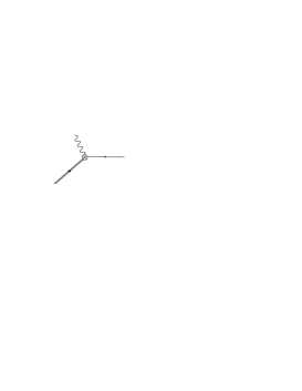
Figure 1: Tree level Feynman diagram for $t\to b+W^{+}$ in both QCD and SCET. Here the double line is an incoming top quark, single line stands for the b quark and the $W$ boson is given by the wavy line.

Now we match QCD amplitude onto the ${\rm SCET}_{\rm I}$ operators to one loop. We calculate the virtual corrections to the ${\rm SCET}_{\rm I}$ current at the order $\alpha_{s}$, then comparing with the QCD amplitude at the same order Campbell:2004prd , we determine the Wilson coefficients and the matching scale $\mu_{H}$, as well. We should expect that the ${\rm SCET}_{\rm I}$ calculations reproduce the infrared divergence in QCD.

Figure 2: QCD virtual corrections to the ${\rm SCET}_{\rm I}$ operator at the order ${\cal O}(\alpha_{s})$. The spring line is a usoft gluon and the collinear gluon are represented by a spring with a line going through.

The leading order QCD virtual corrections to the ${\rm SCET}_{\rm I}$ operator are shown in fig. 2 except for the self energy corrections. Once we ignore the $b$ quark mass, the loop integrals are scaleless and vanish in dimensional regularization. In order to extract ultraviolet divergence, we put $b$ quark offshell here. Evaluating those diagrams in $d=4-2\epsilon$ dimensions gives divergences from usoft vertex correction

$$I_{\rm usoft}=-\frac{\alpha_{s}C_{F}}{4\pi}\,\left(\frac{1}{\epsilon^{2}}-\,\frac{2}{\epsilon}\log\left(-\frac{n\!\cdot\!q}{\mu}\right)\right)\,{\cal O}_{0}\,,$$ (6)

as well as the collinear gluon correction

$$I_{\rm coll}=-\frac{\alpha_{s}C_{F}}{4\pi}\,\left(\,-\frac{2}{\epsilon^{2}}-\frac{2}{\epsilon}+\frac{2}{\epsilon}\,\log\left(-\frac{\bar{n}\!\cdot\!qn\!\cdot\!q}{\mu^{2}}\right)\,\right)\,{\cal O}_{0}\,.$$ (7)

Here, $q$ is the momentum carried by the outgoing $b$ quark.

The summation of the divergent piece should be canceled by the operator counterterm $\delta Z_{\cal O}$ together with the wavefunction counterterms. Since $\delta Z_{t}=\alpha_{s}C_{F}/(2\pi\epsilon)$ and $\delta Z_{b}=-\alpha_{s}C_{F}/(4\pi\epsilon)$ for heavy and collinear quark wavefunction conterterms, respectively, we can extract $\delta Z_{\cal O}$,

$$\delta Z_{\cal O}=\frac{\alpha_{s}C_{F}}{4\pi}\,\left(\frac{1}{\epsilon^{2}}\,+\frac{5}{2\epsilon}-\frac{2}{\epsilon}\log\left(\frac{\bar{n}\!\cdot\!q}{\mu}\right)\,\right)\,.$$ (8)

Thus, in ${\rm SCET}_{\rm I}$ the leading order plus one-loop virtual correction to the differential decay rates is

$$\frac{\mathrm{d}^{2}\Gamma^{\rm I}_{{\rm L}+{\rm V}}}{\mathrm{d}y\mathrm{d}z}\,=\Gamma_{0}\left(1+C_{0}+\frac{C_{1}}{2}\frac{1-r^{2}}{1+2r^{2}}\right)\,\delta(y)\delta(1-z)\,\left(1-\frac{\alpha_{s}C_{F}}{2\pi}\,\left(\frac{1}{\epsilon^{2}}\,+\frac{5}{2\epsilon}-\frac{2}{\epsilon}\log\left(\frac{\bar{n}\!\cdot\!q}{\mu}\right)\,\right)\right)\,.$$ (9)

We see that the ${\rm SCET}_{\rm I}$ result reproduces exactly the same infrared poles in QCD Campbell:2004prd as expected and the matching coefficent $C_{0}$ and $C_{1}$ are

$$C_{0}=\frac{\alpha_{s}C_{F}}{2\pi}\,\left(-\frac{1}{2}\log\frac{\mu^{2}}{m_{t}^{2}}\,\left(\log\frac{\mu^{2}}{m_{t}^{2}(1-r^{2})^{4}}+5\right)-\frac{\pi^{2}}{4}-6\right.$$

$$\left.\hskip 43.05542pt-2{\rm Li}_{2}(r^{2})-2\log^{2}(1-r)^{2}-\frac{1-3r^{2}}{r^{2}}\log(1-r^{2})\,\right)\,,$$

$$C_{1}=\frac{\alpha_{s}C_{F}}{2\pi}\frac{2}{r^{2}}\log(1-r^{2})\,.$$ (10)

We choose the hard matching scale be $\mu_{H}=\bar{n}\!\cdot\!q=m_{t}(1-r^{2})$ to eliminate large logarithms.

Now we turn to the matching between ${\rm SCET}_{\rm I}$ and ${\rm SCET}_{\rm II}$, which will determine the coefficient ${\cal T}(t,z)$ in the fragmenting jet function. The matching is done at decay rate level at the limit $y\to 0$. Thus the coefficient is dominated by those singular terms in this limit.

The diagrams for usoft and collinear real emissions at next-to-leading-order in $\alpha_{s}$ are shown in fig. 3 and fig. 4, respectively. The amplitude square coming from the usoft emission is the same as making the eikonal approximation in QCD which gives

$$|{\cal M}|_{\rm usoft}^{2}=g_{s}^{2}C_{F}|{\cal M}|_{0}^{2}\,\left(\frac{2}{n\!\cdot\!kv\cdot k}-\frac{1}{(v\cdot k)^{2}}\right)\,,$$ (11)

where $k$ is the momentum for the real gluon emitted.

The collinear diagrams can be evaluated using the SCET Feynman rules Bauer:2001prd . However at certain regions of the phase space, for example when $y\to 0$ while $z\to 1$, the collinear gluon momentum $k$ will become usoft and scales like $Q(\lambda^{2},\lambda^{2},\lambda^{2}$) rather than $Q(\lambda^{2},1,\lambda)$. In this regime, the SCET diagrams will include a double power counting. To get rid of double counting, we should subtract the ”zero-bin” contribution Manohar:2007prd from the collinear diagrams. In our case, the zero-bin can be calculated simply by treating the gluon with momentum $k$ in fig. 4 as a usoft mode. After perform the zero-bin subtraction, collinear real emission is given by

$$|{\cal M}|_{\rm coll}^{2}=\,g_{s}^{2}C_{F}|{\cal M}|^{2}_{0}\frac{1}{q_{gb}^{2}}\left(\,\frac{4\bar{n}\!\cdot\!q}{\bar{n}\!\cdot\!k}+(2-2\epsilon)\frac{n\!\cdot\!q}{{n\!\cdot\!q}_{gb}}\,-\frac{4{\bar{n}\!\cdot\!q}_{gb}}{\bar{n}\!\cdot\!k}\,\right)\,,$$ (12)

where $q$ is the $b$ quark momentum and $q_{gb}$ is the total momentum for the $b$ quark-gluon system. The last term in the equation above corresponds to the zero-bin subtraction.

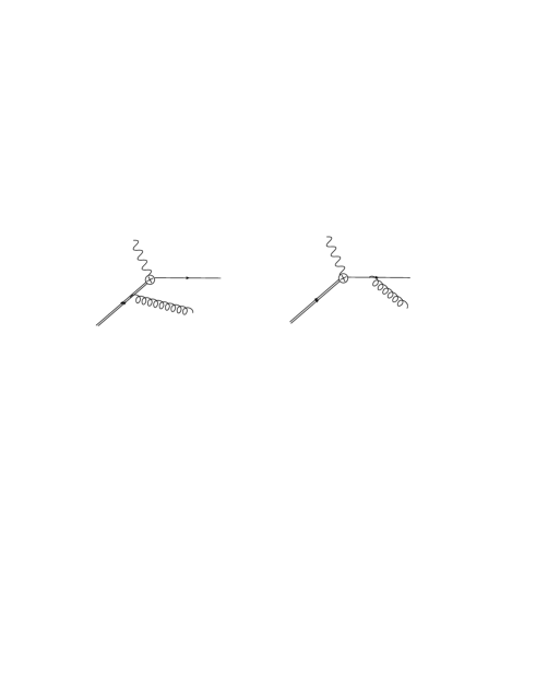
Figure 3: Real emission of a usoft gluon in SCET.

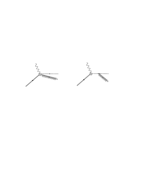
Figure 4: Real emission of a collinear gluon in SCET.

Combining usfot, collinear and zero subtraction, we calculate the differential decay rates in ${\rm SCET}_{\rm I}$, which yields

$$\frac{\mathrm{d}^{2}\Gamma^{\rm I}_{\rm R}}{\mathrm{d}y\mathrm{d}z}\, = \frac{\alpha_{s}C_{F}}{2\pi}\Gamma_{0}|C_{\rm H}|^{2}\,\left(\frac{4\pi\mu^{2}}{m_{t}^{2}(1-r^{2})^{2}}\right)^{\epsilon}\,\frac{(1+r)^{2\epsilon}}{\Gamma(1-\epsilon)}\,z^{-\epsilon}(1-z)^{-\epsilon}\,\left(\frac{y}{y_{max}}\right)^{-\epsilon}\,(y_{max}-y)^{-\epsilon}$$ (13)

$$\times\left[\frac{1}{y}\,\left(\frac{z^{2}+1-\epsilon(1-z)^{2}}{1-z}\right)\,-\frac{2}{(1+r)^{2}}\frac{1}{(1-z)^{2}}\right]\,,$$

where all the hard matching coefficients in Eq. (II) are included in $|C_{\rm H}|^{2}$.

To determine the coefficient ${\cal T}(t,z)$ in the fragmentng jet function, we compare the cross section calculated within ${\rm SCET}_{\rm I}$ and the one in ${\rm SCET}_{\rm II}$. The matching procedure is similar to Ref. Fleming:2006prd . However, in our case, extracting the singular contributions is complicated due to the fact that $y_{max}$ is not linear in $z$. A simple way to do the matching is based on the fact that the fragmenting jet function is universal and in principle itself has no information about the $W$ boson mass, thus, formally this function doesn’t depend on $r$ explicitly. This allows us to set $r$ to $0$ to simplify the calculation. (In this case, $y_{max}=1-z$ which is identical to Ref. Fleming:2006prd ) After obtaining the coefficient ${\cal T}(t,z)$, we then restore the $r$ dependence.

Here, we keep the $r$ dependence explicitly. We slightly generalize the method proposed in Ref. Fleming:2006prd to investigate the singular behavior as $y\to 0$ in Eq. (13) in the Appendix. The virtual corrections to the cross section should also be included to this order. Since the loops are scaleless and thus vanish in dimensional regularization. Therefore the infrared divergent part is the same as minus the counterterm. Once including both real and virtual corrections, we find that in ${\rm SCET}_{\rm I}$

$$\frac{\mathrm{d}^{2}\Gamma^{\rm I}_{{\rm R}+{\rm V}}}{\mathrm{d}y\mathrm{d}z}\, = \frac{\alpha_{s}C_{F}}{2\pi}\Gamma_{0}|C_{\rm H}|^{2}\,\left\{\,\delta(y)\delta(1-z)\left(\,-\log\left(\frac{\mu_{H}^{2}}{\mu^{2}}\right)+\frac{1}{2}\log^{2}\left(\frac{\mu_{H}^{2}}{\mu^{2}}\right)\,-\frac{\pi^{2}}{4}\right)\,\right.$$ (14)

$$\left.+\delta(y)\left[-\frac{1}{\epsilon}P_{qq}(z)\,+\bar{P}_{qq}(z)\log\left(z\right)\,+(1+z^{2})\left(\frac{\log(1-z)}{1-z}\right)_{+}+(1-z)\right]\right.$$

$$\left.-2\left[\kappa\left(\frac{1}{\kappa y}\right)_{+}\,+\kappa\left(\frac{\log(\kappa y)}{\kappa y}\right)_{+}\,\right]\delta(1-z)+\frac{\kappa\mu_{H}^{2}}{\mu^{2}}\left(\frac{1}{\frac{\kappa\mu_{H}^{2}}{\mu^{2}}y}\right)_{+}{\bar{P}}_{qq}(z)\,\right\}\,,$$

where, we define $\kappa=1/(1+r)^{2}$ and $\mu_{H}=m_{t}(1-r^{2})$. We have used the identity Eq. (38) for the plus-prescription in the Appendix. Here

$$P_{qq}(z)=\frac{1+z^{2}}{(1-z)_{+}}+\frac{3}{2}\delta(1-z)=\bar{P}_{qq}(z)+\frac{3}{2}\delta(1-z)\,,$$ (15)

is the quark to quark splitting function.

In ${\rm SCET}_{\rm II}$ the decay rates read as

$$\frac{\mathrm{d}^{2}\Gamma_{\rm II}}{\mathrm{d}y\mathrm{d}z}\,=\Gamma_{0}|C_{\rm H}|^{2}\frac{m_{t}^{2}(1-r)^{2}}{2(2\pi)^{3}}\,\int_{0}^{p_{gb}^{+}}\mathrm{d}k^{+}\int_{z}^{1}\frac{\mathrm{d}x}{x}\,{\cal T}_{bb}\left(\mu_{H}k^{+},\frac{z}{x}\right)D_{b}(x)S_{t}(p^{+}_{gb}-k^{+})\,.$$ (16)

By definition, $p_{gb}^{+}=m_{t}(1-r)/(1+r)y$ and we suprress the scale dependence here. We can perform expansions for those functions involved in the differential decay rates to order $\alpha_{s}$,

$${\cal T}_{bb}(\omega k^{+},z)=2(2\pi)^{3}\left(\,\delta(\omega k^{+})\delta(1-z)\,+\frac{\alpha_{s}C_{F}}{2\pi}{\cal T}_{bb}^{(1)}(\omega k^{+},z)\right)\,,$$

$$S_{t}(k^{+})=\delta(k^{+})+\frac{\alpha_{s}C_{F}}{\pi}S^{(1)}_{t}(k^{+})\,,$$

$$D_{b}(x)=\delta(1-x)-\frac{\alpha_{s}C_{F}}{2\pi\epsilon}P_{qq}(x)\,.$$ (17)

Therefore, omitting the leading term in $\alpha_{s}$, we can manipulate Eq. (16) to the form

$$\frac{\mathrm{d}^{2}\Gamma^{(1)}_{\rm II}}{\mathrm{d}y\mathrm{d}z}\,=\,\frac{\alpha_{s}C_{F}}{2\pi}\Gamma_{0}|C_{\rm H}|^{2}\left[\,\delta(y)\frac{-P_{qq}(z)}{\epsilon}\,+2\delta(1-z)(\kappa\mu_{H})S_{t}^{(1)}(\kappa\mu_{H}y)\,+(\kappa\mu^{2}_{H}){\cal T}_{bb}^{(1)}(\kappa\mu_{H}^{2}y,z)\right]\,.$$ (18)

The shape function here is the same as the one in $B$ meson decay which has been calculated in Ref. Bauer:2000prd . We follow their procedure to get

$$(\kappa\mu_{H})S_{t}^{(1)}(\kappa\mu_{H}y) = \delta(y)\left(-\frac{1}{2}\log\left(\frac{\mu_{H}^{2}}{\mu^{2}}\right)\,+\frac{1}{4}\log^{2}\left(\frac{\mu_{H}^{2}}{\mu^{2}}\right)\,-\frac{\pi^{2}}{24}\,\right)\,$$ (19)

$$\hskip 8.61108pt-\kappa\left(\frac{1}{\kappa y}\right)_{+}\,-\kappa\left(\frac{\log(\kappa y)}{\kappa y}\right)_{+}\,-\frac{\kappa\mu_{H}^{2}}{\mu^{2}}\,\left(\frac{\log(\frac{\kappa\mu_{H}^{2}}{\mu^{2}}y)}{\frac{\kappa\mu_{H}^{2}}{\mu^{2}}y}\right)_{+}\,.$$

Plugging Eq. (19) into Eq. (18) and comparing with the decay rate in ${\rm SCET}_{\rm I}$ Eq. (14), we can derive the coefficient ${\cal T}_{bb}$

$${\cal T}^{(1)}_{bb}(t,z)=\,\delta(t)\left(\,\bar{P}_{qq}(z)\log(z)+(1+z^{2})\left(\frac{\log(1-z)}{1-z}\right)_{+}+(1-z)-\frac{\pi^{2}}{6}\delta(1-z)\right)$$

$$\hskip 64.58313pt+\frac{1}{\mu^{2}}\left(\frac{1}{t/\mu^{2}}\right)_{+}\bar{P}_{qq}(z)+\,\frac{2}{\mu^{2}}\left(\frac{\log(t/\mu^{2})}{t/\mu^{2}}\right)_{+}\delta(1-z)\,.$$ (20)

Here $t=\kappa\mu_{H}^{2}y$ is the invariant jet mass. Requiring all large logarithms to vanish, the intermediate matching scale should be set to the jet mass, $\mu_{c}^{2}=t$. And we see from Eq. (II) that formally the matching coefficient can not depend on $r$ as we explained before. We can check that after integrating Eq. (II) over $z$, we recover the massless collinear quark jet function at order $\alpha_{s}$ in SCET.

III Running

The differential decay rate has several well separated scales $\mu_{H}$, $\mu_{c}$ and $\mu_{s}$ involved. To go from one scale to another, we use the renormalization group equation to sum up large logarithms. First the ${\rm SCET}_{\rm I}$ operators are run from hard scale $\mu_{H},$ using the ${\rm SCET}_{\rm I}$ RGEs, down to the collinear scale $\mu_{c}$ at which ${\rm SCET}_{\rm I}$ is matched onto ${\rm SCET}_{\rm II}$. Then we run the shape function to the scale $\mu_{s}=\mu_{c}^{2}/\mu_{H}$.

There are several ways to perform this procedure Leibovich:2000prd ; Becher:2006prl ; Fleming:2008prd . We choose to do the running in the moment space then by take the inverse Mellin transform to obtain a resummed decay rate Leibovich:2000prd . In the moment space the formula for the decay rate could be written as

$$\Gamma_{N}=\Gamma_{0}|C_{H}(\mu_{c})|^{2}\int_{z}^{1}\frac{\mathrm{d}x}{x}\,\hat{{\cal T}}\left(\frac{z}{x},N,\mu_{c}\right)D_{b}(x,\mu_{c})\,\hat{S}_{t}(N,\mu_{s})\,.$$ (21)

To obtain the moment space decay rate above, we first normalize the fragmenting jet function and the shape function in a way that both functions are dimensionless quantities, which we use hats to represent for. We define a variable $\bar{y}=1-y$ and the moments are taken respect to $\bar{y}$. Also we introduce $u$ to express $k^{+}$ in Eq. (16) in terms of $\kappa\mu_{H}(1-u)$. In the regime $y\to 0,{\bar{y}}\to 1$, large $N$ limit is achieved. In moment space, the scales are $\mu_{c}=\mu_{H}\sqrt{\kappa}/\sqrt{\bar{N}}$ and $\mu_{s}=\kappa\mu_{H}/\bar{N}$. The hard scale $\mu_{H}$ is the same as defined in the previous section.

At the collinear scale $\mu_{c}$, the large logarithms in the matching coefficient $\hat{{\cal T}}$ vanish, which gives

$$\hat{{\cal T}}(z,N,\mu_{c})=\delta(1-z)+\frac{\alpha_{s}C_{F}}{2\pi}\,\left(\log(z){\bar{P}}_{qq}(z)\,+(1+z^{2})\left(\frac{\log(1-z)}{1-z}\right)_{+}\,+(1-z)\,\right)\,.$$ (22)

The only $N$ dependence are through $\mu_{c}$ in the strong coupling $\alpha_{s}$.

Now we take another Merlin transform respect to $z$,

$$\Gamma_{NM}=\Gamma_{0}|C_{H}(\mu_{c})|^{2}\,\left(1+\frac{\alpha_{s}(\mu_{c})C_{F}}{2\pi}T(M)\right)D_{b}(M,\mu_{c})\hat{S}_{t}(N,\mu_{s})\,.$$ (23)

The running of the fragmentation function $D(M,\mu)$ in the moment space is given by

$$\mu\frac{\mathrm{d}}{\mathrm{d}\mu}D(M,\mu)=\,\frac{\alpha_{s}}{4\pi}a(M)D(M,\mu)\,.$$ (24)

The leading order solution is then

$$D(M,\mu_{c})=D(M,\mu_{H})\,\exp\left(\frac{a(M)}{2\beta_{0}}\log(1-\chi)\right)\equiv\,D(M,\mu_{H})\exp\left(h_{M}(\chi)\right)\,,$$ (25)

with $\chi=\log(\bar{N}/\kappa)\alpha_{s}(\mu_{H})\beta_{0}/4\pi$ and $\beta_{0}=(11C_{A}-2n_{f})/3$. To the leading order, the running of the combination $\alpha_{s}C_{F}/(2\pi)T(M)D(M,\mu)$ satisfies similar equation as Eq. (25) with $a(M)$ replaced by $4a(M)-2\beta_{0}$. Therefore, we can define $h^{\prime}_{M}(\chi)$ in the same way as $h_{M}(\chi)$ and have

$$\frac{\alpha_{s}(\mu_{c})C_{F}}{2\pi}T(M)D(M,\mu_{c})=\frac{\alpha_{s}(\mu_{H})C_{F}}{2\pi}T(M)D(M,\mu_{H})\exp(h^{\prime}_{M}(\chi))\,.$$ (26)

All $M$ dependence has been moved into factor $h_{M}$ and $h^{\prime}_{M}$.

The running of the ${\rm SCET}_{\rm I}$ currents along with the shape function could be lifted from Ref. Fleming:2006prd . We obtain the following resummed decay rate in the moment space:

$$\Gamma_{NM} = \Gamma_{0}|C_{H}(\mu_{H})|^{2}e^{\log(N/\kappa)g_{1}(\chi)+g_{2}(\chi)}\,\hat{S}_{t}(N,\mu_{s})$$ (27)

$$\hskip 51.6665pt\times\left(e^{h_{M}(\chi)}+e^{h^{\prime}_{M}(\chi)}\frac{\alpha_{s}(\mu_{H})C_{F}}{2\pi}T(M)\right)D_{b}(M,\mu_{H})\,,$$

where

$$g_{1}(\chi)=-\frac{2\Gamma_{1}}{\beta_{0}\chi}\left[\,(1-2\chi)\log(1-2\chi)-2(1-\chi)\log(1-\chi)\,\right]\,,$$

$$g_{2}(\chi)=-\frac{8\Gamma_{2}}{\beta_{0}^{2}}\left[\,-\log(1-2\chi)+2\log(1-\chi)\right]$$

$$\hskip 34.44434pt\,-\frac{2\Gamma_{1}\beta_{1}}{\beta_{0}^{3}}\left[\,\log(1-2\chi)-2\log(1-\chi)+\frac{1}{2}\log^{2}(1-2\chi)\,-\log^{2}(1-\chi)\right]$$

$$\hskip 34.44434pt\,+\frac{4\gamma_{1}}{\beta_{0}}\log(1-\chi)+\frac{2B_{1}}{\beta_{0}}\log(1-2\chi)$$

$$\hskip 34.44434pt\,-\frac{4\Gamma_{1}}{\beta_{0}}\log n_{0}\left[\log(1-2\chi)-\log(1-\chi)\right]\,,$$ (28)

with $n_{0}=e^{\gamma_{E}}$ and

$$\Gamma_{1}=4C_{F}\,,\hskip 21.52771pt\Gamma_{2}=C_{A}\left[C_{A}\left(\frac{67}{36}-\frac{\pi^{2}}{12}\right)-\frac{5n_{f}}{18}\right]\,,$$

$$B_{1}=-4C_{F}\,,\hskip 21.52771pt2\gamma_{1}=-\frac{3}{2}C_{F}\,,$$

$$\beta_{1}=\left(\frac{34}{3}C_{A}^{2}-\frac{10}{3}C_{A}n_{f}-2C_{F}n_{f}\right)\,.$$ (29)

Evaluating the inverse Mellin transform with respect to $N$ using the results of Ref. Leibovich:2000prd shows that

$$\frac{\mathrm{d}\Gamma_{M}}{\mathrm{d}y} = \,\Gamma_{0}|C_{H}(\mu_{H})|^{2}\int_{1-y}^{1}\frac{\mathrm{d}u}{u}\hat{S}_{t}\left(\frac{1-y}{u}\right)\left[\,-u\frac{\mathrm{d}}{\mathrm{d}u}\,\left(\theta(1-u)\frac{e^{lg_{1}(l)+g_{2}(l)}}{\Gamma\left[\,1-g_{1}(l)-lg_{1}^{\prime}(l)\right]}\,\right.\right.$$ (30)

$$\hskip 38.74988pt\times\left.\left.\left(e^{h_{M}(l)}+e^{h^{\prime}_{M}(l)}\frac{\alpha_{s}(\mu_{H})C_{F}}{2\pi}T(M)\right)D_{b}(M,\mu_{H})\,\right)\,\right]\,,$$

where $l=-\alpha_{s}\beta_{0}/(4\pi)\log(1-u)$ and $g_{1}^{\prime}(l)=\mathrm{d}g_{1}(l)/\mathrm{d}l$. The factor $h_{M}(l)$ can be eliminated using Eq. (25)

$$e^{h_{M}(l)}D(M,\mu_{H})=\exp\left[\frac{a(M)}{2\beta_{0}}\log(1-l)\right]D(M,\mu_{H})=D(M,\kappa\mu_{H}\sqrt{1-u})\,,$$ (31)

and the same thing holds for $h^{\prime}_{M}(l)$.

After eliminating both factors $h_{M}$ and $h^{\prime}_{M}$, all the $M$ dependence is now entirely included in the moments of the fragmentation function, so the inverse Mellin transform with respect to $M$ is straightforward. Hence we derive the resummed decay rate:

$$\frac{\mathrm{d}^{2}\Gamma}{\mathrm{d}y\mathrm{d}z}\, = \Gamma_{0}|C_{H}(\mu_{H})|^{2}\,\int_{1-y}^{1}\frac{\mathrm{d}u}{u}\hat{S}_{t}\left(\frac{1-y}{u}\right)\left[\,-u\frac{\mathrm{d}}{\mathrm{d}u}\,\left(\theta(1-u)\frac{e^{lg_{1}(l)+g_{2}(l)}}{\Gamma\left[\,1-g_{1}(l)-lg_{1}^{\prime}(l)\right]}\,\right.\right.$$ (32)

$$\hskip 38.74988pt\times\left.\left.\left(\delta(1-z)+\frac{\alpha_{s}C_{F}}{2\pi}\tilde{T}^{(1)}(z)\right)\otimes D_{b}(z,\kappa\mu_{H}\sqrt{1-u})\,\right)\,\right]\,,$$

where the convolution is defined as $f\otimes g=\int_{z}^{1}\mathrm{d}x/xf(x)g(x/z)$ and $\tilde{T}^{(1)}(z)$ is the second term in Eq. (22). We note that in the second line the $\alpha_{s}$ has an scale dependence on $\kappa\mu_{H}\sqrt{1-u}$ which has been suppressed. Due to the universality of the fragmenting jet function, Eq. (32) can also be applied to other processes like heavy meson decay $B\to XK\gamma$ and etc. When applying Eq. (32), we should be careful in dealing with the Landau poles since the functions $g_{i}(l)$ blow up as $u$ approach $1$. A simple way to avoid Landau pole is to set an upper limit on $u$. And it has been argued that the difference between integrating to this upper limit $u_{max}$ and to one is of order power suppressed corrections Leibovich:2001plb .

IV Summary

We have discussed the top quark doubly differential decay rate near the phase space boundary where the $W$ boson carries its maxim energy within the framework of soft collinear effective theory. The factorization theorem for top quark decay is similar to the one for $B\to XK\gamma$, in which a novel fragmenting jet function arises in replacement of the standard parton fragmentation function. The fragmenting jet function provides information on the invariant mass of the jet from which a detected hadron framents. In this work we calculated the fragmenting jet function to next-to-leading order in $\alpha_{s}$ by comparing the decay rates calculated in ${\rm SCET}_{\rm I}$ and ${\rm SCET}_{\rm II}$. We also check the relation between our derived fragmenting jet function with the inclusive collinear quark jet function, finding that they satisfy ${\cal J}(t)\to{\cal G}(t,z)\mathrm{d}z$ as indicated in Ref. Procura:2010prd . We use the renormalization group equation to sum up large logarithms involved in the decay rates. After resummation, we arrive at an analytic formula for the distribution. Our results can be applied to other heavy hadron decay processes with a detected light hadron like $B$ meson radiative decay. And the result of this work may help tuning event generators such as Herwig.

APPENDIX

In this section, we show how to extract contributions which are singular as $y\to 0$. And for this reason we will drop all terms which are regular in this limit.

First we consider the combination of the form

$$I_{1}[y,z]\equiv(1+r)^{2\epsilon}\,y^{-1-\epsilon}\,\frac{y_{max}^{\epsilon}(y_{max}-y)^{-\epsilon}}{(1-z)^{1+\epsilon}}\,.$$ (33)

where $y_{max}=(1+r)^{2}z(1-z)/(z+r^{2}(1-z))$.

We start with considering the integration

$$\int_{z_{min}}^{z_{max}}\mathrm{d}zI_{1}[y,z]\left(g(z)-g(1)\right)\,+g(1)\int_{z_{min}}^{z_{max}}\mathrm{d}zI_{1}[y,z]\,,$$ (34)

with $z_{max}=1-1/(1+r)^{2}y+{\cal O}(y^{2})$ and $z_{min}={\cal O}(y)$. So $z_{max}$ goes to $1$ as $y$ goes to $0$ while $z_{min}$ approaches to $0$ in this limit.

Due to the distributional identity,

$$\frac{1}{y^{1+\epsilon}}=-\frac{1}{\epsilon}\delta(y)\,+\left(\frac{1}{y}\right)_{+}\,-\epsilon\left(\frac{\log y}{y}\right)_{+}\,,$$ (35)

the non-singular contributions as $y\to 0$, including the integration limits, in the first term of Eq. (34) could be expanded around $y=0$ and leaves out all terms of order ${\cal O}(y)$ or higher. Thus the first term becomes

$$(1+r)^{2\epsilon}\,y^{-1-\epsilon}\,\int_{0}^{1}\mathrm{d}z\frac{g(z)-g(1)}{(1-z)^{1+\epsilon}}\,$$

$$\hskip 25.83325pt=(1+r)^{2\epsilon}\,y^{-1-\epsilon}\,\int_{0}^{1}\mathrm{d}z\left[\left(\frac{1}{1-z}\right)_{+}\,-\epsilon\left(\frac{\log(1-z)}{1-z}\right)_{+}\right]g(z)\,.$$ (36)

Using the distributional identity and expand in $\epsilon$ gives that

$$\int_{z_{min}}^{z_{max}}\mathrm{d}zI_{1}[y,z]\left(g(z)-g(1)\right)$$ (37)

$$= \int_{0}^{1}\mathrm{d}z\left\{\delta(y)\left[-\frac{1}{\epsilon}\left(\frac{1}{1-z}\right)_{+}\,+\left(\frac{\log(1-z)}{1-z}\right)_{+}\right]\,+\kappa\left(\frac{1}{\kappa y}\right)_{+}\left(\frac{1}{1-z}\right)_{+}\right\}g(z)\,.$$

Here $\kappa=1/(1+r)^{2}$ and we have applied the relation

$$\kappa\left(\frac{\log^{n}(\kappa y)}{\kappa y}\right)_{+}=\,\frac{\log^{n+1}(\kappa)}{n+1}\delta(y)\,+\sum_{k=0}^{n}\frac{n!}{(n-k)!k!}\log^{n-k}(\kappa)\,\left(\frac{\log^{k}(y)}{y}\right)_{+}$$ (38)

Now we turns to the second term in Eq. (34) by considering a further integration

$$\int_{0}^{1}\mathrm{d}y\int_{z_{min}}^{z_{max}}\mathrm{d}z\,I_{1}[y,z]\left(f(y)-f(0)\right)+f(0)\int_{0}^{1}\mathrm{d}y\int_{z_{min}}^{z_{max}}\mathrm{d}zI_{1}[y,z]\,.$$ (39)

Since the first term in the equation above is finite as $y\to 0$. We can set $\epsilon=0$ and then perform the integration over $z$, which results in

$$\int_{0}^{1}\mathrm{d}y\int_{z_{min}}^{z_{max}}\mathrm{d}z\,I_{1}[y,z]\left(f(y)-f(0)\right)$$

$$\hskip 25.83325pt=-\int_{0}^{1}\mathrm{d}y\frac{1}{y}\,\log\left(\frac{1-z_{max}}{1-z_{min}}\right)\,\left(f(y)-f(0)\right)$$

$$\hskip 25.83325pt=-\int_{0}^{1}\mathrm{d}y\,\kappa\left(\frac{\log(\kappa y)}{\kappa y}\right)_{+}f(y)\,.$$ (40)

The last equation is obtained by expanding $z_{max}$ and $z_{min}$ around $y=0$, e.g., $\log(1-z_{max})=\log(\kappa y(1+{\cal O}(y)))=\log(\kappa y)+{\cal O}(y)$, and ignore all the non-singular contributions in $y$.

Evaluating the integration of the second term in Eq. (39) gives

$$f(0)\int_{0}^{1}\mathrm{d}y\int_{z_{min}}^{z_{max}}\mathrm{d}zI_{1}[y,z]=\left(\frac{1}{2\epsilon^{2}}-\frac{\pi^{2}}{12}\right)f(0)\,.$$ (41)

Gathering all the pieces, we have

$$\int_{z_{min}}^{z_{max}}\mathrm{d}zI_{1}[y,z]g(z)$$ (42)

$$= \int_{0}^{1}\mathrm{d}z\left[\,\delta(y)\left(\,\left(\frac{1}{2\epsilon^{2}}-\frac{\pi^{2}}{12}\right)\delta(1-z)\,-\frac{1}{\epsilon}\left(\frac{1}{1-z}\right)_{+}\,+\left(\frac{\log(1-z)}{1-z}\right)_{+}\,\right)\right.$$

$$\left.+\kappa\left(\frac{1}{\kappa y}\right)_{+}\,\left(\frac{1}{1-z}\right)_{+}\,-\kappa\left(\frac{\log(\kappa y)}{\kappa y}\right)_{+}\delta(1-z)\right]g(z)\,.$$

Next we consider another integration which will contribute to the non-singular part as $y$ goes to $0$

$$\int_{z_{min}}^{z_{max}}\mathrm{d}zI_{2}[y,z]g(z)\,=\frac{2}{(1+r)^{2-2\epsilon}}\,y^{-\epsilon}\int_{z_{min}}^{z_{max}}\mathrm{d}z\,\frac{y_{max}^{\epsilon}(y_{max}-y)^{-\epsilon}}{(1-z)^{2+\epsilon}}\,g(z)\,.$$ (43)

We note that here $g(z)$ can be replaced by $g(1)$ since those terms behave like $\int\mathrm{d}1/(1-z)\propto\log(y)$ are non-singular.

Then we use

$$\int_{0}^{1}\mathrm{d}y\int_{z_{min}}^{z_{max}}\mathrm{d}z\,I_{2}[y,z](f(y)-f(0))\,+f(0)\int_{0}^{1}\mathrm{d}y\int_{z_{min}}^{z_{max}}\mathrm{d}zI_{2}[y,z]\,$$

$$\hskip 25.83325pt=\frac{2}{(1+r)^{2}}\,\int_{0}^{1}\mathrm{d}y\int_{z_{min}}^{z_{max}}\mathrm{d}z\,\frac{1}{(1-z)^{2}}(f(y)-f(0))\,+f(0)\int_{0}^{1}\mathrm{d}y\int_{z_{min}}^{z_{max}}\mathrm{d}zI_{2}[y,z]$$

$$\hskip 25.83325pt=\int_{0}^{1}\mathrm{d}y\left(2\kappa\left(\frac{1}{\kappa y}\right)_{+}\,\delta(1-z)-\frac{1}{\epsilon}\delta(y)\delta(1-z)\right)f(y)\,.$$ (44)

Again, we have expand $z_{max}$ and $z_{min}$ around $y=0$ and throw away regular contributions.

Therefore

$$\int_{z_{min}}^{z_{max}}\mathrm{d}zI_{2}[y,z]g(z)$$ (45)

$$= \int_{0}^{1}\mathrm{d}z\,\left(-\frac{1}{\epsilon}\delta(y)\delta(1-z)\,+2\kappa\left(\frac{1}{\kappa y}\right)_{+}\delta(1-z)\right)g(z)\,.$$