SNIF: A Futuristic Neutrino Probe for Undeclared Nuclear Fission Reactors

Abstract

Today reactor neutrino experiments are at the cutting edge of fundamental research in particle physics. Understanding the neutrino is far from complete, but thanks to the impressive progress in this field over the last 15 years, a few research groups are seriously considering that neutrinos could be useful for society. The International Atomic Energy Agency (IAEA) works with its Member States to promote safe, secure and peaceful nuclear technologies. In a context of international tension and nuclear renaissance, neutrino detectors could help IAEA to enforce the Treaty on the Non-Proliferation of Nuclear Weapons (NPT). In this article we discuss a futuristic neutrino application to detect and localize an undeclared nuclear reactor from across borders. The SNIF concept proposes to use a few hundred thousand tons neutrino detectors to unveil clandestine fission reactors. Beyond previous studies we provide estimates of all known background sources as a function of the detector’s longitude, latitude and depth, and we discuss how they impact the detectability.

I Neutrinos and Proliferation

In a context of increasing carbon-free emission energy needs, civilian nuclear energy will probably expand all over the world. Globalization, as well as the goal of energy independence, led to an increase of the list of countries aiming to acquire technological know-how in the field of nuclear energy. As a consequence of the spread of practical knowledge, the possibility of diverting a nuclear facility towards non-civilian use could increase in the next 50 years. The main duty of the United Nations’ International Atomic Energy Agency (IAEA) is to work to make sure that nations use nuclear energy only for peaceful purposes aieawww . Apart from political difficulties regarding safeguards, the efficiency of IAEA controls may be limited by monitoring techniques in the future due to the fast growth of nuclear facilities around the world. Since 2003, the Department of Safeguards of the International Atomic Energy Agency has been evaluating the potential applicability of neutrino detection technologies for safeguard purposes.

In 2008, a transverse working group of reactor neutrino experts from the Member States together with the IAEA Division of Technical Support (SGTS) firmly established that neutrino detectors have unique abilities to non intrusively monitor a nuclear reactor’s operational status, power and fissile content in real-time, from outside the reactor containment. This led to the definition of three safeguards scenarios of interest. The first two, the confirmation of the absence of unrecorded production of fissile material in declared reactors and the estimation of the total burn-up of a reactor core, are related to the so-called near-field applications with detectors located a few tens of meters from the core. The third scenario concerns clandestine or undeclared nuclear reactor detection with core-detector distances ranging from tens to hundreds of kilometers, also known as far-field applications.

As far as near-field monitoring is concerned, a few detectors specifically built for safeguards have shown robust, long term measurements of these metrics in actual installations at operating power reactors songs ; nucifer . Several experimental programs aiea2008report are currently being carried out in Brazil, France, Italy, Japan, Russia and the United States, guided by IAEA inputs on their needs at specific reactors. Over a longer time scale, it has been recognized that neutrino detectors could have a considerable value in bulk process and safeguards by design approaches for new and next generation reactors. Concerning far-field applications, an undeclared reactor operating secretly would stand out in the received $\bar{\nu}_{e}$. Such a detection possibility has already been discussed in learned ; guillian , using a network of gigantic water Cherenkov detectors (of 1 million tons each) being deployed below four kilometers of water in deep oceans.

The purpose of this article is to address the possibility of detecting undeclared nuclear reactors across borders with very large neutrino detectors, outlining basic principles and figures regarding the deployment of large neutrino detectors as a safeguard tool.

Our study revisits the detectability of clandestine nuclear reactors with a comprehensive treatement of known neutrino sources and backgrounds. In this article we consider as a baseline case a 10³⁴ free protons liquid scintillator detector fitting inside an oil supertanker. The strategy presented in this article is to deploy one or more of these detectors as close as possible to a suspicious area, typically between 100 and 500 km. The detectors are then temporarily sunk underwater for data taking until a significant amount of events are detected. Our baseline operating time is 6 months.

We will first introduce the reactor neutrino field in section II. In section III we review the neutrino technology and we outline the detector design in section IV. We then compute the known neutrino sources (section V) and backgrounds (section VI). We then establish the rogue activity detection criteria in section VII. In section VI we study non-neutrino backgrounds in order to derive and possibly relax the minimum operation depth with respect to previous studies guillian . We also provide a method for determining the location of an undeclared reactor (section VIII). We conclude by addressing the feasibility of the concept within the next thirty years.

II Reactor neutrinos

II.1 Neutrino production

Fission reactors are prodigious producers of neutrinos, emitting about $10^{21}$ $\bar{\nu}_{e}$ $\mathrm{s}^{-1}$ $\mathrm{GW}_{\rm th}^{-1}$. In this article we will only consider the electron antineutrinos emitted by $\beta$-decays, referred to simply as neutrinos in the rest of the text. In actual light water reactors, the Uranium fuel is enriched to a few percent in ²³⁵U. The fission of ^235,238U and ^239,241Pu isotopes produces neutron rich nuclei which must shed neutrons to approach the valley of stability. The beta decays of these fission products produce approximately six electron antineutrinos per fission. Measurements for ²³⁵U and ^239,241Pu and theoretical calculations for ²³⁸U are used to evaluate the $\bar{\nu}_{e}$ spectrum Schreckenbach:1985ep ; Hahn:1989zr ; lm2010 . Since ²³⁸U only contributes to about 11% of the neutrino signal, and further since the error associated is less than 10%, ²³⁸U contributes less than 1% to the overall uncertainty in the $\bar{\nu}_{e}$ flux. The overall normalization is known to about $1.4\%$ Declais and its shape to about $2\%$ Bugey . As a nuclear reactor operates, the proportions of the fissile elements evolve with time. During a typical fuel cycle the Pu concentrations increase, so the total neutrino flux decreases with time. As an approximation we use a typical averaged fuel composition during a reactor cycle corresponding to the following fission fractions: ²³⁵U (55.6%), ²³⁹Pu (32.6%), ²³⁸U (7.1%) and ²⁴¹Pu (4.7%).

II.2 Neutrino oscillations

There is now compelling evidence for flavor conversion, also known as oscillations, of atmospheric, solar, reactor and accelerator neutrinos SK98 ; osc2 ; osc3 ; sno ; KamLAND1 ; K2K ; Minos . Thus reactor neutrino experiments measure a rate weighted by the survival probability $P(\bar{\nu}_{e}\rightarrow\bar{\nu}_{e})$ of the $\bar{\nu}_{e}$ emitted by nuclear power stations at a distance (L), resulting in a deviation from the $1/L^{2}$ dependence that would otherwise be expected.

Reactor neutrino oscillations depend on the atmospheric $\Delta m_{31}^{2}$ and the solar $\Delta m_{21}^{2}$ mass splittings between the three neutrino mass eigenstates, as well as the three mixing angles $\theta_{12}$, $\theta_{23}$, and the small, still undetermined $\theta_{13}$ PDG . In this article, we consider minimum baselines of about 100 km. Because $\Delta m_{sol}^{2}\ll\Delta m_{atm}^{2}$ and because of the smallness of $\theta_{13}$, the oscillation probability can be approximated by:

$$1-P(\bar{\nu}_{e}\rightarrow\bar{\nu}_{e})=\sin^{2}(2\theta_{12})\,\sin^{2}\left(1.27\frac{\Delta m_{21}^{2}[{\rm eV}^{2}]L[{\rm m}]}{E_{\bar{\nu}_{e}}[{\rm MeV}]}\right)\>$$

For energies above 1.8 MeV, the survival probability is close to 1 for distances of 0 to several tens of kilometers. The survival probability then oscillates around an asymptotic value of 0.57 as the distance ranges from about 50 km to 300 km. At further distances, much larger than the ’solar-driven’ oscillation length, the probability is practically very close to 0.57. In this work we treat neutrino oscillation with the state-of-the-art three neutrino oscillations formula PDG , but we set $\theta_{13}$ to 0 since its small value will not impact the oscillation probability for the purpose of this study.

Because of the combination of MeV range energies and baselines less than $10^{3}$ km the modification of the oscillation probability induced by the coherent forward scattering from matter electrons is less than a few percent. In this work the effect is small enough to be neglected.

II.3 Neutrino rate

The mean energy released $\left<E_{f}\right>$ per fission is around 205 MeV kopeikin . The energy-weighted cross section to detect neutrinos amounts to $\left<\sigma_{f}\right>=5.8\times 10^{-43}$ cm² per fission. The reactor thermal power ($P_{\rm th}$) is related to the number of fissions per second ($N_{f}$) by $N_{f}=6.24\times 10^{18}\;{\rm s}^{-1}\,P_{\rm th}[{\rm MW}]/\left<E_{f}\right>[{\rm MeV}]$. The neutrino interaction rate ($R_{L}$) at a distance $L$ from the source, assuming no neutrino oscillations, is then $R_{L}=N_{f}\left<\sigma_{f}\right>n_{p}/(4\pi L^{2})$, where $n_{p}$ is the number of hydrogen atoms, or free protons, of the target. The expected neutrino rate from clandestine reactors at a few hundred kilometers is quite small, due to the weak neutrino interaction cross section and the $1/L^{2}$ dependence. Neglecting neutrino oscillations, a 100 MW_th reactor would induce 450 events per year in a $10^{34}$ proton detector at a distance of 100 km. In this particular case, neutrino oscillations induce a deviation from the $1/L^{2}$ dependence and only 250 neutrino events could effectively be detected as shown on Figure 1.

Figure 1: Number of events detected in 1 year in a detector with $10^{34}$ protons, as a function of the distance from a single 100 MW reactor. The dashed line shows the variation in the absence of neutrino oscillations, while the full line shows the actual observation taking into account oscillations. From 50 km to 100 km a caracteristic ’wiggle’ can be seen. Beyond 250 km, oscillations simply cause a reduction in the flux, but the $1/L^{2}$ dependence is restored.

Therefore the target mass must at least be of the order of a hundred thousand tons. For fundamental research, neutrino detectors as large as 50,000 tons have been built SK98 . A few projects of larger liquid scintillators detectors, like lena ; hanohano , are currently being discussed.

II.4 Clandestine reactors

We define clandestine or rogue reactors as nuclear reactors not declared by a country to the international community (IAEA). Like regular research or power reactors they would be copious sources of neutrinos. We assume such reactors to have the same features as regular reactors, though their nuclear thermal power is unknown. In this article we will consider that clandestine reactors may have powers between 10 MW_th to 2 GW_th. We consider the fuel composition of clandestine reactors to be similar to the composition of commercial reactors, on average. This assumption has no strong impact on the detectability of clandestine activity since the neutrino rate depends mainly on the thermal power.

III Neutrino detection

Electron antineutrinos can be detected via inverse beta decay on free protons: $\bar{\nu}_{e}+p\to e^{+}+n$ for $E_{\bar{\nu}_{e}}>E_{\rm thr}\sim 1.8$ MeV, and their energy is derived from the measured positron kinetic energy as $E_{\bar{\nu}_{e}}\simeq E_{e^{+}}+E_{\rm thr}$. We call visible energy the energy deposited in the detector, corresponding to $E_{\rm vis}=E_{e^{+}}+2m_{e}$. The inverse beta decay cross section has been precisely computed in VogelBeacom . A neutrino event is thus characterized by a prompt positron event which deposits a visible energy between 1 and 8 MeV, followed by a delayed gamma event arising from neutron capture within $\tau\sim 10-200\;\mu$s. The minimal energy of 1 MeV of the prompt event is caused by the positron’s annihilation in the active volume. Prompt and delayed event are spatially correlated, within $<1\;{\rm m}^{3}$. They both have a $\beta/\gamma$-type pulse shape, distinguishable in liquid scintillators. This signature allows to discriminate efficiently against backgrounds.

Water-Cherenkov and liquid scintillator detectors allow real-time spectroscopy of electron antineutrinos.

Liquid scintillators have commonly been used for the past 60 years to detect neutrinos using the inverse $\beta$-decay reaction. The hydrogen atoms serve as targets to neutrinos, producing ionizing particles. The liquid scintillator emits light in the UV-range when crossed by these charged particles. These liquids can be flammable or dangerous to the environment and thus require special care when large amounts are handled. The inverse beta-decay reaction does not allow to recover the direction of the incoming neutrino, apart from a slight backward shift of the positron angular distribution. The scintillation light, isotropically emitted, allows to find the position of the neutrino interaction within a few tens of centimeters. Large volume detectors may yield a few hundred photoelectrons per deposited MeV, corresponding to an energy resolution of a few percent even for the less energetic neutrinos. This detection technology based on liquid scintillator has the capability to measure the full $\bar{\nu}_{e}$ spectrum since the instrumental threshold may be lowered to 1 MeV or less, depending on backgrounds.

High purity water is also used as a detection medium for charged particles traveling through at super-luminous speed SK98 , inducing so-called Cherenkov radiation. Water has a few advantages: it is straightforward to handle, non flammable, non toxic, available in large volumes at relatively low cost, and easily purified by common techniques to improve its transparency. For charged particles above an energy threshold (0.78 MeV for electrons) only 200 UV photons/cm are emitted along the track, i.e. roughly 30 times less light than liquid scintillators. Similarly this detection technique cannot be used to determine the direction of the incoming neutrino.

For both technologies, doping the liquid with Gadolinium at the level of 1–5 g/l can greatly improve the sensitivity to electron antineutrinos from reactors. The large cross section for neutron capture on ¹⁵⁷Gd ($2.59\,10^{5}$ barn) and ¹⁵⁵Gd ($6.1\,10^{4}$ barn) enhances the sensitivity to the delayed neutron signal. The positron, emitting scintillation photons or radiating Cherenkov photons, is immediately detected with or without Gadolinium. However the neutron, quickly thermalized in the hydrogen-rich media, is captured on Gd with a probability of more than 80%. Upon capturing a neutron, a Gadolinium nucleus relaxes to its ground state by emitting a cascade of gamma rays having a total energy of about 8 MeV, thus enhancing the detection efficiency. This is especially true in water where the neutron capture signal on hydrogen, at 2.2 MeV, is barely detectable above backgrounds. Furthermore the time delay between the positron and neutron events is significantly decreased, leading to a reduction of accidental backgrounds. Unlike Gadolinium-doped water, stable Gadolinium-doped liquid scintillators are difficult to obtain, but we assume that current technologies being developed for the next generation of experiments Cras2005 will be routinely available thirty years from now.

In both cases visible-UV light is collected by photomultiplier tubes covering the walls of the detector vessel. The total charge and photon arrival times allow to reconstruct the incident neutrino’s energy and interaction time.

IV Detector design

In this section we briefly describe our baseline detector design and address the technical challenges in realizing a SNIF detector module. Our design concept is similar to those developed for large neutrino detectors proposed for fundamental research, such as Titand titand , Hano-Hano hanohano and LENA lena .

We consider a detector module containing $10^{34}$ free protons (fiducial volume). This corresponds to 138,000 tons of linearalkylbenzene ($\text{LAB},{\rm C}_{18}{\rm H}_{30}$) based liquid scintillator, contained in a volume of 160,000 m³ (density of 0.86). This could be hosted in a cylindrical tank of 23 m radius and 96.5 m length. Optical coverage of the detector walls of 20 percent would require 17,000 photomultipliers of the Superkamiokande type (20 inches). Depending on the total muon rate in the module, and thus on the operating depth, the fiducial volume could be optically segmented. This huge detector module has to be designed to be transportable and deployable in the deep ocean. We propose to host the detector in a supertanker to be transported on the detection site. By comparison, a modern supertanker can have a capacity of over 400,000 deadweight tons. It would then be immersed at a depth of a several hundred to several thousand meters.

In the rest of the article we will focus our discussion on liquid scintillator technology. The components of the detector are embedded in each other, the liquid scintillator being in the central volume. Linearalkylbenzene is currently used in neutrino experiments (for instance SNO+ sno+ , Double Chooz dc , Daya Bay dayabay ) because of its good optical transparency ($>$ 20 m), its high light yield, its low amount of radioactive impurities, and its high flash point (140 degrees Celsius) which makes safe handling easier. Moreover experimental studies of temperature and pressure dependence validated its performance in deep underwater environment hanohano .

Scintillator timing properties as well as optical transparency are improved by adding a combination of solutes, typically PPO (a few g/l) and bisMSB (a few mg/l). In addition, the neutron capture capability of the scintillator would be greatly enhanced with the dissolution of a Gadolinium complex (a few g/l typically). This should be considered as a serious option if long term stability issues are solved. It would require dedicated surface treatement of the inner walls, such as Teflon coating.

Such a liquid scintillator medium would lead to 80% neutrino detection efficiency. Setting an analysis threshold at $E_{\rm vis}>2.6$ MeV would greatly reduce the material radiopurity constraints, simplifying industrial production of the modules (see Section VI.1). We thus consider this energy cut in our baseline scenario, and account for the resulting loss of efficiency.

In order to further reduce backgrounds the inner stainless steel tank could be enclosed in another steel vessel providing a protective layer of ultra pure water against external radioactivity. This 1 meter thick region could be equiped with phototubes detecting Cherenkov light from cosmic muons, allowing to further suppress the muon-induced background (see Section VI.3.2). This would imply the installation of 4,000 additional phototubes on the outer tank walls.

The geometry of both tanks should be curved to accommodate the deep-sea hydrostatic pressure. The detector should finally be zero-buoyant to be sunk into the deep ocean for its operation and to be brought back to the surface for maintenance or redeployment elsewhere.

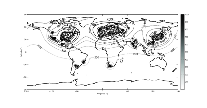
Figure 2: Maps illustrating the number of neutrino events that would be detected in a $10^{34}$ free protons detector ($E_{\rm vis}>2.6$ MeV, 4,000 m operating depth) after half a year of data taking. 201 nuclear power stations have been included, accounting for a 78% global load factor on averaged. This map includes all non-neutrino backgrounds which are negligible at this depth in the northern hemisphere (see Section VI).

V Known neutrino sources

In this section we review the two largest sources of known neutrinos. These sources are an irreducible background for the search of undeclared nuclear cores: power/research reactor neutrinos and geological neutrinos. As a first step the known sources neutrino signal should be subtracted from the observed rate to unveil undeclared nuclear fission activity.

V.1 World nuclear power stations

Clandestine reactor and commercial reactor neutrinos are totally indistinguishable. Neutrinos from commercial plants are thus an irreducible source of background that could overwhelm the clandestine signal. However this background is predictable since the IAEA can access all power plants’ geographical coordinates, thermal power, and operating status at any time. In our simulation, we included 201 nuclear power stations, most of them having multiple units. They amount to 1,134 GW_th total thermal power. The reactor’s latitude and longitude were checked to a precision of one hundredth of a degree, using satellite views via Google Earth®. The mean load factor of each reactor for the 1998-2008 period has been included when possible. We consider that the global power is stable, though reactors will be turning on and off for refueling and maintenance. We assume that the day-by-day thermal power would be knowable by the monitoring authorities, with a 3% uncertainty. This is consistent with what present day experiments, KamLAND and Borexino, are able to achieve kamlandOsc2008 ; borexinogeonu . We also assume an averaged isotopic composition for all cores known within 3% uncertainty.

The number of events detected in 6 months in a SNIF detector module as a function of geographical position on Earth is shown on Figure 2. Most of the commercial nuclear power stations are located in the northern hemisphere, mainly belonging to developed countries, especially the United States of America, Europe, and Japan. These three zones gather more than 85% of the total world nuclear power budget. Only four power stations are present in the southern hemisphere, in Argentina, Brazil, and South Africa, amounting to only 14 GW_th. This asymmetry plays an important role in the sensitivity of the neutrino method. Obviously it is harder to detect clandestine activity in areas where commercial and/or research reactor activity is high.

In this work we consider only power reactors with thermal power greater than 100 MW_th, and we do not account for research reactors. This is justified because the total power produced by commercial nuclear reactors is far greater than that of research reactors. Though this assumption is correct for most locations around the world, it may be locally inexact in some areas with no power stations.

V.2 Geoneutrinos

Geoneutrinos are natural electron antineutrinos arising from the decay of radioactive isotopes of Uranium, Thorium, and Potassium in the crust and mantle of the Earth. The spectrum of neutrinos from the decay chains of Uranium and Thorium extends above the energy threshold for inverse neutron decay (1.8 MeV) to the maximum geologic neutrino energy (3.27 MeV), corresponding to a 2.5 MeV visible energy deposition in a liquid scintillator detector. Potassium neutrinos are below threshold for this reaction. For the current study we used a $2^{\circ}\times 2^{\circ}$ map providing the Uranium and Thorium geoneutrino fluxes based on the Earth reference Model in mantovanibse . Geoneutrino fluxes are computed following the prescription described in geonurate , at the detector’s longitude and latitude coordinates, taking neutrino oscillations into account. The geoneutrino background rate ranges from a few hundred interactions per 10³⁴ H.year in the middle of the oceans (thin oceanic crust), to a few thousand interactions per 10³⁴ H.year in the middle of the continents (thick continental crust). A possibility to discard this background completely is to set an analysis threshold above 2.5 MeV. Another possible source of background a hypothetical natural nuclear reactor of a few TW in the core of the Earth georeactor . In our study we neglect its potential influence.

VI Non-neutrino backgrounds

Irreducible commercial reactor neutrinos are not the only source of backgrounds. Non-neutrino backgrounds could prevent any neutrino detection if not handled carefully since the expected low signal (clandestine minus known activity) must not be drowned in a high rate of background events. This implies extensive passive shielding to protect the fiducial volume from natural radioactivity, as well as active shielding to veto cosmic rays. In addition a thickness of hundreds to thousands meters of water is mandatory to achieve sufficient supression of atmospheric muons, neutrons and cosmogenic radioisotopes. In this section we review the available detection technologies. We then provide a model for the three main kinds of non-neutrino backgrounds: accidental coincidences, fast neutrons and the long-lived muon induced isotopes ⁹Li/⁸He, as a function of the operating depth.

VI.1 Accidental backgrounds

When detecting neutrinos, naturally occurring radioactivity (U, Th, K) of the component of the detector may create fake signal - so-called accidental background - defined as a coincidence of a prompt energy deposition between 1 and 10 MeV, followed by a delayed neutron-like event, occurring after a delay $\tau_{d}$ of a few hundredths of a millisecond, in close proximity to the prompt energy deposit (within a volume $V_{d}\sim 1\,\mathrm{m}^{3}$). With these notations, the accidental background rate $r_{acc}$ is given by $r_{acc}\sim r_{p}\;r_{d}\;\tau_{d}\;V_{d}\;V_{det}$, where $r_{p}$ and $r_{d}$ are the specific background rates (in units of s^-1m^-3) for the prompt and the delayed signal, respectively. $V_{det}$ is the total detection volume.

The potentially most dangerous of these backgrounds are those caused by radioactive impurities within the active detection liquid. The use of standard techniques like distillation, water extraction, nitrogen purging, and column chromatography allows to achieve sufficiently low concentrations in radio–impurities kamland0307030 ; borexino08 . The detection liquid is contained in a vessel and photomultipliers catch the light emitted in the neutrino interaction. Those materials and equipments also contain radioactive impurities whose decay products may release their energy within the liquids. The selection of high purity materials entering the detector (mechanical structures, photomultiplier tubes) as well as passive shielding provide an efficient tool against this type of background. Surface/wall-induced events could be rejected through spatial reconstruction cuts, with a loss of fiducial volume however. Taking accidental backgrounds into account leads to the detector design presented in Section IV.

Figure 3: Background rate as a function of the detector depth in meters of water equivalent for an exposure of $10^{34}$ H.year. Fast neutron and cosmogenic backgrounds are estimated with the models presented in sections VI.3.2 and VI.3.1. For comparison we indicate our estimates of accidental backgrounds for two different thresholds, 1 and 2.6 MeV (visible energy). We also give three possible estimates for the geoneutrino rates, for continental crust areas (high), coastal areas (medium), and oceanic crust areas (low) hanohano . Known neutrino sources under three hypotheses are also displayed for comparison (see section V).

In Table 1 we present our background rescaling results. We use the $r_{p}$ and $r_{d}$ values measured in Borexino and KamLAND, thus the accidental background rate in SNIF scales with $V_{det}$ only. We rescale the estimated rates for a $10^{34}$ H.y (proton.year) target immersed in deep water (SNIF baseline design). Choosing the Borexino extrapolation providing the lowest estimate, we note the accidental background dominates the cosmogenics backgrounds at depths below 2,000 m, as displayed on Figure 3. This choice is justified assuming a detector as radiopure as Borexino could be achievable at the SNIF scale within the next 30 years. Considering no scaling of the delayed signal background may be too simplistic, however. In order to get a more robust result in our current study we get rid of the accidental background contribution by setting an analysis threshold $E_{\rm vis}>2.6$ MeV. This implies a loss of signal statistics of 28%, but it also relaxes the radiopurity constraints by orders of magnitude, simplifying the project feasibility.

Experiment	KamLAND	Borexino	SNIF extrapolated from
Label			KamLAND	& Borexino
Flat eq. depth	2,050 m	3,050 m	2,500 m
Scintillator	${\rm C}_{11.4}{\rm H}_{21.6}$	${\rm C}_{9}{\rm H}_{12}$	${\rm C}_{16}{\rm H}_{30}$
H/m3	$6.60\;10^{28}$	$5.30\;10^{28}$	$6.24\;10^{28}$
C/m3	$3.35\;10^{28}$	$3.97\;10^{28}$	$3.79\;10^{28}$
density	0.78	0.88	0.86
Mass (tons)	912	278	138,000
Volume (m3)	1170	316	160,000
Radius (m)	6.5	4.25	23
Cyl. Length (m)	—	—	96.5
$\mu-$Section (cm2)	$1.3\;10^{6}$	$0.57\;10^{6}$	$4.4\;10^{7}$
$\mu-$Flux (cm-2s-1)	$1.6\;10^{-7}$	$0.3\;10^{-7}$	$0.7\;10^{-7}$
$\mu-$Energy (MeV)	219	276	247
$\mu-$Rate (s-1)	$2.13\;10^{-1}$	$1.6\;10^{-2}$	3.0
$\mu-$DT (200 $\mu$s)	$4\;10^{-5}$	$0.3\;10^{-5}$	$60\;10^{-5}$
Co-DT (200 ms)	$4\;10^{-2}$	$0.3\;10^{-2}$	$60\;10^{-2}$
Exposure (H.y)	$2.44\;10^{32}$	$6.02\;10^{30}$	$10^{34}$
Threshold (MeV)	0.9	1	0.9	1
Accidental Rate	80.5$\pm$0.1	0.08$\pm$0.001	3,300$\pm$4	133$\pm$2
Li/He Rate	7.0$\pm$1	0.03$\pm$0.02	85.9$\pm$12.2	108$\pm$71.9
Fast n Rate	9$\pm$9	0.025$\pm$0.025	171$\pm$17	93.4$\pm$9
Geo-$\nu$	69.7	2.5$\pm$0.2	2,860	4,150$\pm$332
Reactor-$\nu$	1,609$\pm$51	5.7$\pm$0.3	65,900$\pm$2,080	9,460$\pm$498

Table 1: Breakdown of the background estimates for SNIF. We consider two different background measurements from the KamLAND and Borexino neutrino searches kamlandOsc2008 ; borexinogeonu ; Cosmogenics from KamLAND are rescaled from kamlandCosmo2010 . $\mu-$DT and Co-DT are the estimates of both muon and cosmogenics induced dead time (DT). The flat equivalent depths are taken from meihime . Extrapolation to SNIF corresponds to a 10³⁴ proton detector operating for 1 year at a depth of 2,500 m, according to the prescription given in hagner2000 ; meihime . In this table, SNIF is taken to be located at the KamLAND/Borexino sites to calculate Geo- and Reactor-neutrino backgrounds. Geo-neutrino rates are measured, in agreement with the reference Earth model bse .

VI.2 Cosmic muons induced dead time

The cosmic-ray muon flux underwater can be deduced from data at different depths and extrapolated as a function of equivalent water depth where $10^{5}$ g/cm² = 1,000 mwe (meters of water equivalent). Using the depth–intensity relation for the total muon flux with a flat overburden given in meihime , we derive the muon rate in a detector containing $10^{34}$ free protons having a section exposed to muons of $1.48\;10^{8}\;{\rm cm}^{2}$ (cylinder of r=23 m radius and l=96.5 m length). At water depths of 500 m, 1,000 m, 2,000 m, and 4,000 m we obtain a muon rate of 560, 110, 8, 0.3 Hz, respectively. Vetoing the detector for 200 $\mu$s after each muon would thus lead to respective muon-induced dead times of 11%, 2.2%, 0.15%, and 0.006%. From this data we derive the minimum operating depth our module at around 0.5 km, not yet accounting for background. We include this depth-dependent dead time in our sensitivity estimates. Reducing the detector’s dead time at shallower depth is possible by subdividing the module in optically decoupled compartments.

Figure 4: Maps illustrating the neutrino and non-neutrino background events that would be detected in a $10^{34}$ free protons detector (1 MeV energy threshold), operating for half a year at a depth of 2,500 m. At distances greater than 1,000 kilometers from nuclear power station clusters, the rate is dominated by geoneutrino events (see Section V.2). This background could be rejected by setting an analysis threshold $E_{\rm vis}>2.6$ MeV.

VI.3 Correlated backgrounds

Cosmic ray muons will be the dominating trigger rate at the depth of our detectors. Their very high energy deposition corresponds to about 2 MeV per centimeter path length and provides thus a strong discrimination tool. They induce the main source of dangerous events, cosmogenic activity and fast neutrons, which mimic the neutrino signal.

VI.3.1 Muon induced cosmogenic activity

Energetic muons can interact with carbon nuclei and produce by spallation radioactive isotopes such as ⁸He, ⁹Li and ¹¹Li. These nuclei are unstable and decay emitting an electron and a neutron, thus perfectly mimicking the signal from an antineutrino interaction ; moreover the long lifetimes of these nuclei, a few 100 ms, complicate the task of identifying them since they occur long after the muons that created them. This background is considered to be the most serious difficulty to overcome in the SNIF concept, and drives the operating depth of the detector. When this background is reduced - roughly below 3,500 m of water - ⁸He, ⁹Li and ¹¹Li decays could be identified through a four-fold coincidence ($\mu\to n\to\beta\to n$) characteristic signature.

In order to estimate the cosmogenic backgrounds we used the rates experimentally measured by the Kamland kamlandCosmo2010 and Borexino borexinogeonu collaborations. The main detector features as well as muon induced backgrounds are provided in Table 1. The production rate of cosmogenic radioisotopes is proportional to the muon flux ($\Phi_{\mu}$), the cross section $\sigma_{tot}(E_{\mu})\sim E^{0.73}_{\mu}$ hagner2000 , and the total number of carbon nuclei. We start from the muon flux predictions at the flat equivalent overburden of the KamLAND (2050 m of water equivalent) and Borexino (3,050 m of water equivalent) locations. We then rescale the backgrounds to $10^{34}$ H.year for different depths according to the total muon flux, and energy formulae given in meihime . Estimates are corrected according to the different carbon composition in Borexino, KamLAND and SNIF liquid scintillators. Results for a $10^{34}$ H.year target deployed at a depth of 2,500 m are presented in Table 1. An additional selection of events with $E_{\rm vis}>2.6$ MeV would reject 23% of the cosmogenic background, according to the simple spectrum shape presented in mention . In this work we envisage a further possibility of eradicating the cosmogenics backgrounds by vetoing the detector after each muon for a long enough time. We veto a 3-m-radius cylinder around each muon track for 600 ms (3 times the ⁸He, ⁹Li decay time periods). Neglecting the veto inefficiency we find that this technique could only be effective at operating depth greater than 1,500 m to preserve a dead time below 10% in a 138,000 ton detector. We thus neglect the cosmogenics backgrounds from this depth on. Below 1,500 m we considered the KamLAND rescaling from kamlandCosmo2010 . The evolution of the predicted cosmogenics background in SNIF with respect to the detector depth is presented on Figure 3.

For completeness we note that a water Cherenkov detector is less affected by this specific background sksolar because of the lower yield of these nuclei when spallation reactions occur with oxygen nuclei.

VI.3.2 Muon induced fast neutron activity

An important source of background comes from neutrons produced in the surrounding of the detector by cosmic ray muon induced hadronic cascades. The difficulty is that the primary cosmic ray muon may not penetrate the detector, being thus invisible. This is especially true for a small detector. These processes produce arbitrarily high energy neutrons inducing proton recoils mimicking the prompt signal, and then producing the coincident neutron signal after thermalization and capture. Such a sequence can mimic a $\bar{\nu}_{e}$ event. At several hundred meters of water equivalent, muon-induced neutron production can be fairly well estimated from the results of previous underground experiments, like KamLAND kamlandOsc2008 and Borexino borexinogeonu . Fast neutrons can indeed be produced by muons either crossing the inner stainless steel vessel or interacting in the water around the detector. We estimate the rate of fast neutrons by scaling the KamLAND and Borexino results according to the procedure described in Section VI.3.1. Results for a $10^{34}$ proton.year target deployed at a depth of 2,500 m are presented in Table 1. An additonal selection of events with $E_{\rm vis}>2.6$ MeV would reject 31% of the fast neutrons background, assuming a flat energy spectrum.

For SNIF we only consider the case of Borexino and we reduce the neutron production from the rock (4/5 of the total rate) by a factor of 2.7 in order to correct for the lower density of water. Contrary to smaller detectors like KamLAND and Borexino, in very large detectors like SNIF the fast neutron background could be considered as a surface background. We thus assume that the fast neutrons induced by muons crossing the bulk of the detector could be perfectly tagged in a very large liquid scintillator detector (neglecting tiny veto inefficiencies). The dominant fast neutron component induced by the water surrounding the detector can only be detected at distances less than 3 meters from the detector inner vessel walls. Further inside the detector fast neutrons will have been significantly slowed. This lowers the estimated background by 70%. The evolution of our predicted fast neutron rate with respect to the detector depth is depicted on Figure 3. We assume an uncertainty of 10%, achievable within the next 30 years.

VII Detecting a clandestine activity

In this section we detail the statistical method used to decide whether a signal of undeclared activity is seen above the known sources and backgrounds, at a given confidence level.

VII.1 Defining a decision threshold

Let $b$ be the background, i.e. the average number of events occurring in the detector in the absence of any clandestine activity. Either from past measurements, or theoretical calculations or other input, $b$ is known with a certain uncertainty $\sigma_{b}$. We will treat this error as Gaussian. Now let $o$ be the number of events actually observed in the detector. The first question one can ask is whether $o$ is compatible with a fluctuation of the background, or whether it is too high and could therefore be a sign of suspicious activity. This is a well known problem, studied in great details in e.g. currie . We will simply reproduce some of the explanations and calculations therein. Following Currie’s notation, we will write $L_{C}$ the decision threshold or critical level: it is the observed number of events above which the operator will declare having observed a positive signal, i.e. detected a possible clandestine reactor. Of course this level depends on the rate of false alarms (incorrect reported detection while no clandestine reactor is present, also known as type I error) that one is willing to tolerate a priori.

In the absence of any clandestine reactor, $o$ follows a Gaussian distribution, with mean $b$ and error $\sqrt{b+\sigma_{b}^{2}}$. Given a certain confidence level $\alpha$,

$$o<b+k_{\alpha}\sqrt{b+\sigma_{b}^{2}},$$

where $k_{\alpha}$ is the $\alpha$ quantile of the normal distribution. Consequently,

$$L_{C}=k_{\alpha}\sqrt{b+\sigma_{b}^{2}}.$$ (1)

If, having observed $o$ events, $o-b>L_{C}$, then the detector will report the presence of a clandestine reactor, with a pre-determined false alarm rate $1-\alpha$.

This criterion has the advantage of being directly applicable to data, and is used to make a decision on whether to take further action. It depends solely on the mean and uncertainty on the background, and the chosen confidence level. Note that at this stage there is no localization of the detector. The purpose of $L_{C}$ is to decide whether the observation signals suspicious activity or not. With the definition above, $L_{C}$ is a number of events. If the distance from the reactor is known, $L_{C}$ can be converted to a power (see section II.3): this power is the maximum power that would yield a signal consistent with the background. We will often convert $L_{C}$ to either power or distance in what follows. Conversely, if the power of the clandestine reactor is known, we can use the considerations of section II.3 to convert $L_{C}$ to a maximum distance below which the operator would declare having observed a positive signal.

VII.2 Defining a detection limit

Following currie , we can also determine $L_{D}$, the minimum detectable signal, viz. the minimal amount of signal that could a priori be detected. For this purpose it is first necessary to determine $L_{C}$ at a certain false alarm rate $\alpha$, as explained in the previous section. We then define a second confidence level $\beta$, controlling the amount of type II error that we tolerate: $\beta$ is the probability that an existing reactor would be missed by our method. With these definitions, $L_{D}$ is the average amount of signal that would lead to detection (i.e. observation of more than $L_{C}$ counts) with probability $1-\beta$. The solution to this problem is found in currie :

$$L_{D}=L_{C}+\frac{k_{\beta}^{2}}{2}\left(1+\sqrt{1+\frac{4L_{C}}{k_{\beta}^{2}}+4\frac{L_{C}^{2}}{k_{\alpha}^{2}k_{\beta}^{2}}}\right).$$ (2)

With these two quantities, we can explore the sensitivity of our detection method. As for $L_{C}$, $L_{D}$ can either be converted to a power (if the distance from the reactor is known) or to a distance (if the power of the reactor is known). At known distance, the resulting power is the minimum power detectable a priori with type I and II error rates of $\alpha$ and $\beta$ respectively. At known power, the resulting distance is the maximum distance at which this power would a priori be detected, with type I and II error rates of $\alpha$ and $\beta$ respectively.

VII.3 Impact of known nuclear reactors

In this section we study $L_{C}$ and $L_{D}$ (or their conversions to power/distance), as a function of the detector mass, exposure time, clandestine reactor thermal power, and the known nuclear reactor neutrino rate at any Earth location.

Let us introduce a new luminosity unit, called the r.n.u. (for reactor neutrino unit) and defined as $1~{}\text{r.n.u.}=0.197\;10^{30}~{}\text{MeV}$. With this unit, an experiment taking data for $T$ years with a total clandestine nuclear power of $P$ GW_th. and with $N\;10^{34}$ free protons inside the target has a luminosity ${\cal L}=T\,P\,N~{}\text{r.n.u.}$ The expected number of events, $N(L)$, at a distance $L$ from a reactor, assuming no - oscillation, is

$$\begin{split}N(L)=&\frac{\left<\sigma_{f}\right>}{4\pi\left<E_{f}\right>}\frac{\cal L}{L^{2}}\simeq 230\;\left(\frac{T}{0.5\text{[y]}}\right)\\ &\left(\frac{P}{100\text{[MW]}}\right)\left(\frac{N}{10^{34}}\right)\left(\frac{1}{L\text{[km]}^{2}}\right)\end{split}$$ (3)

The rate in equation 3 is then corrected for neutrino oscillations in all our calculations.

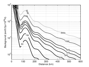
Figure 5: Clandestine nuclear reactor power (MW) detectable with the neutrino method accounting only from known neutrino sources. (left) Maximum power (in MW) of an undeclared nuclear reactor consistent with the known neutrino sources as a function of the reactor distance (km) and neutrino rate from commercial nuclear power stations, as described in section VII.1. We set a 10% false alarm tolerance. (right) Minimum power (in MW) of an undeclared nuclear reactors that could a priori be detectable by the neutrino method as a function of the neutrino background and the reactor distance (km), as described in section VII.2. The false alarm rate is 10% and the probability of missing an existing reactor is 10%. We consider an exposure of $0.5\;10^{34}$ H.y. Wiggles in the range 50-150 km are due to neutrino oscillations.

Figure 2 shows the neutrino rate world map at an operating depth of 4,000 m. Correlated backgrounds, as described in Section VI, turn out to be negligible at this depth. We apply a 2.6 MeV visible energy threshold, rejecting accidental and geoneutrino backgrounds. Three representative cases of the commercial reactor neutrino rate levels can be identified: a low rate area, the southern hemisphere, where the detector would detect $<500$ events in 6 months, a medium rate area corresponding to $500-1,000$ events, and a high rate area corresponding to $>1,000$ events or more, near clusters of nuclear power stations in Europe, Japan, and North America.

Figure 5 (left) provides the maximum power of an undeclared nuclear reactor consistent with the known neutrino sources. The graphics reads as follows: the horizontal axis is the distance between the hypothetical clandestine reactor and the neutrino detector, the vertical axis is the known neutrino rate from commercial nuclear power stations that could be related to an Earth location. The lines represent the iso-power (MW) contours quantifying the maximum power consistent with the known sources. In all what follows we set a 10% false alarm tolerance (type I error) as described in Section VII.1. In medium background conditions we note that a 300 MW reactor could be inferred after 6 months of observation with a single 138,000 ton liquid scintillator detector located 300 km away.

Figure 5 (right) provides the minimum power of a nuclear reactor detectable by the neutrino method as a function of the neutrino background and the clandestine reactor distance. The probability of missing an existing reactor, or type II error as described in Section VII.2, is set to 10% for the rest of this article.

VII.4 Impact of non reactor neutrino backgrounds

In this section we discuss for the first time the impact of the geoneutrinos and non-neutrino backgrounds on the sensitivity of the neutrino method to detect undeclared nuclear fission activities.

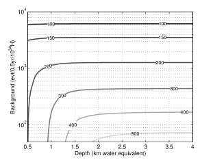
Figure 6: Impact of the non-neutrino backgrounds on the sensitivity to undeclared nuclear fission activity. The horizontal axis provides the operating depth of the neutrino detector, in kilometers of water (kme). The vertical axis represent the known neutrino source rate, for an exposure of $0.5\;10^{34}$ H.y. Assuming a 300 MW undeclared reactor the panel contours describe the iso-minimum distances (km) at which the signal from the clandestine reactor is consistent with the expectation. At closer distances the neutrino detector could tag the clandestine activity. The right panel shows the maximum distance (km) at which one could a priori verify the consistency of the signal with the 300 MW reactor hypothesis.

The map of Figure 4 illustrates the background rates at a depth of 2,500 m that would arise by lowering the detection threshold to 1 MeV (visible energy). This can be compared with Figure 2. At distances of more than a thousand kilometers from nuclear power station clusters the rate is dominated by geoneutrino events. Extrapoling from Figure 5 (left) we see that geo-neutrinos would prevent the detection of any reactor of $<$1 GW with a detector located at $>$ 300 km in the $medium$ commerical neutrino rate regions. This further justifies the choice of setting a 2.6 MeV visible energy threshold.

The influence of backgrounds on the sensitivity to rogue activity is illustrated on Figure 6, as a function of the operating depth and of the expected neutrino rate from nuclear power stations. In this case we assume the existence of a 300 MW rogue reactor. We first notice that for known neutrino source rates of more than a few thousand events the sensitivity is weakly affected by the operating depth below 500 mwe since the non-neutrino background rate remains a small fraction of the total neutrino-like rate.

The evolution of the clandestine activity detectability with respect to the operating depth is illustrated on Figure 6 (left). In medium background conditions we note that a 300 MW reactor could be inferred after 6 months of observation with a single 138,000 ton liquid scintillator detector located 300 km away, only if the depth is greater than 1,500 m. We note that the detection distance would be degraded to 200 km at a depth of 600 mwe. According to our background model we conclude it is not necessary to deploy a detector module below 2,000 m. This is one of the main results of this article.

Figure 7: Remote surveillance of low power research reactors with five $10^{34}$ free protons detector modules operating for one year. The left panel shows the iso-maximum power lines (MW) consistent with expectation, as a function of the detector-reactor distance (km) and the known reactor neutrino rate. The right panel describes the iso-minimum distance contours (km) at which a 75 MW rogue reactor is consistent with all background expectation as a function of the detector depth (km) and known reactor neutrino rate.

VII.5 Scaling up the detection volume

Having developed a compehensive background model we now study the limitation of the neutrino method by scaling up the exposure. This could be done either by enlarging the size of the detector modules, or by operating several detector modules simultaneously, or by increasing the operating period. The potential application could be the surveillance of low power research reactors of a few tens of MW. Let us consider an exposure of $5\times 10^{34}$ H.year, ten times more than our baseline case. This could be realized with five detector modules of 138,000 tons operating for 1 year. Results not considering non-neutrino backgrounds are displayed on Figure 7 (left). For a typical southern hemisphere location (3,000 events from known neutrino sources) we conclude that this system would be sensitive to a 50 MW reactor from a distance of 200 km. The right panel of Figure 7 (left) shows how the sensitivity evolves with the operating depth, still allowing the detection of a 75 MW reactor at a distance of 150 km with detectors operating under 750 m.

VIII Clandestine reactor localization

The strategy developed in this article is to deploy a detector as close as possible to a suspicious area to find evidence of clandestine activity. If any evidence of clandestine activity is found, additional detectors have to be deployed with the objective of finding the clandestine reactor’s location. Four detector modules (i=1,2,3,4) operating at four distinct locations at longitude and latitude ($\lambda$,$\phi$)_i with a positive decision threshold are necessary to isolate a unique location, inferring in addition the reactor’s power. We present here a simple optimization algorithm providing an approximate position of the presumed clandestine reactor as well as confidence levels of the clandestine reactor location, for the best fitted thermal power. For simplicity we assume the reactor to be constantly running.

Let’s assume the presence of an undeclared reactor with a power P (MW) at a location ($\lambda$,$\phi$)_R. S_i is the neutrino signal induced by the rogue reactor in the detector $i$, drawn according to a Poissonian distribution of mean S_i. B_i is the expected background, including known neutrino sources as well as non-neutrino backgrounds. Background uncertainties are taken from Sections V and VI and are added in quadrature. O_i is the observed value in the detector $i$, following a Gaussian of variance O_i (statistical error). The triplet ($\lambda$,$\phi$,P)_R is estimated by minimizing the $\chi^{2}$ function:

$$\chi^{2}=\sum_{i}\frac{(O_{i}-S_{i}(\lambda,\phi,P)_{R}-B_{i})^{2}}{B_{i}+S_{i}(\lambda,\phi,P)_{R}}+\frac{(P-P_{exp})^{2}}{\sigma_{Pexp}^{2}}$$ (4)

$P_{exp}$ and $\sigma_{Pexp}$ are set to 300 MW and 50 MW respectively; in practice they would be set to values that best represent typical rogue reactors.

With four detectors the $\Delta\chi^{2}$ function follows a $\chi^{2}$ distribution with 3 degrees of freedom. However we fit the thermal power at each point on the contour map, allowing to derive the ($\lambda$,$\phi$)_CL confidence intervals at the CL=68.3% (1$\;\sigma$) and CL=95.4% (2$\;\sigma$) by selecting respectively the $\Delta\chi^{2}=\chi^{2}(\lambda,\phi)-\chi_{min}^{2}$=2.30 and 6.18 areas (2 degrees of freedom since $P_{R}$ is fitted at every location). The second term on the right-hand side disfavors large powers inconsistent with low power reactors. It eliminates degenerate solutions located too far away from the region of interest. Any further information providing the thermal power would greatly enhance the localization algorithm, with a possible reduction of the number of detectors.

We notice here that a measurement of the neutrino energy spectrum distorsion due to neutrino oscillations in the undeclared reactor’s spectrum observed with a detector located 70–150 km away could improve the precision of the localization. This effect, already measured by the KamLAND detector kamlandOsc2008 , would however require much higher statistics from the undeclared reactor. We will thus neglect it in our study.

The accuracy and robustness of the method depends on the geographical location of the rogue activity. We now consider three distinct cases: a penisula, an island, and a flat shore. Though the true latitude and longitude coordinates of our examples are hidden they correspond to real cases. In each case the reactor is placed at the origin of each of our coordinate system. In each case the known neutrino sources amount of several hundreds of counts per $10^{34}$ H.y corresponding to intertropical zones.

VIII.1 Peninsula

The first case assumes a 300 MW_th clandestine reactor located on a peninsula. Four detectors are deployed 1,000 m underwater 209 to 264 km away from the clandestine reactor. They operate for 1 year. Known reactor neutrino rates provide 631 events in each detector on average, to be compared with a mean rogue signal of 76 events. The clandestine reactor is clearly detected by three of the four modules (see Table 2).

($\lambda$,$\phi$)	Distance	$<$S$>$	$<$B$>$	O	$L_{c}$	O-$<$B$>$
(-1.0∘,+1.6∘)	209 km	101	643	749	54	106
(+0.1∘,+2.1∘)	234 km	86	645	714	54	69
(+2.6∘,+0.2∘)	286 km	52	628	627	53	-1
(+1.3∘,-2.0∘)	264 km	63	610	714	53	104

Table 2: Four detectors (each containing 10³⁴ free protons) are operating undersea at a depth of 1,000 m, for 1 year, about $250$ km away from a 300 MW clandestine reactor located on a peninsula. S is the rogue signal. B is the sum of the counts from known nuclear reactors and non-neutrino backgrounds. O is the observed value according to a random experimental trial. $L_{c}$ is the decision threshold value. $O-L_{c}>B$ is the detection criteria.

Figure 8 demonstrates the ability to detect and locate the 300 MW_th clandestine reactor with four detector modules located at an average distance of 250 km.

Figure 8: Localization of a clandestine reactor located on a peninsula. Four detectors (squares) surround a 300 MW_th reactor (diamond). The triangle shows the reconstructed position at the best fitted power. The 68.3% (1 $\;\sigma$) and 95.4% (2$\;\sigma$) confidence levels are displayed. The thermal power at best fit is $P=429$ MW_th.

In order to assess the perfomances of the neutrino method we draw 1,000 random trials of the peninsula experiment at various detector operating depths: 500, 750, 1,000, 1,500, 2,500 and 3,500 mwe. We then reconstruct the reactor’s position and power. Figure 9 illustrate the reconstruction of the reactor position with a detector immersed under 1,500 mwe. The spatial resolution, estimated as the 68% quantile of the distance between the best fit position and the true position, is $D_{68\%}$=55 km. Similarily the mean reconstructed thermal power is 241$\pm$44 MW. Results are various depth are presented on Table 4.

Figure 9: Distribution of the distance (km) between the true and the reconstructed positions for 1,000 trials of the peninsula experiment. In this particular case the detectors operate at a depth of 1,500 m. The position is reconstructed within $D_{68\%}$=55 km (dark gray area) in 68% of the cases.

VIII.2 Island

The second case assumes a 300 MW_th clandestine reactor located on an island. Four detectors are deployed at a depth of 1,000 m, between 156 and 235 km from the clandestine reactor. They operate for 1 year. All the known neutrino sources provide 750 events on average, to be compared with a mean rogue signal of 127 events. The clandestine reactor is unambiguously detected by the four modules (see Table 3). In the example displayed on Figure 10 its position is well reconstructed, a few tens of kilometers from the true location. The thermal power is well estimated, at 288 MW, attesting to the potential performance of the neutrino method in a favorable case where detectors surround the suspicious location.

($\lambda$,$\phi$)	Distance	$<$S$>$	$<$B$>$	O	$L_{c}$	O-$<$B$>$
(+1.5∘,+1.5∘)	235 km	86	772	816	57	44
(0∘,-1.4∘)	156 km	221	707	886	55	179
(-2.0∘,0∘)	221 km	94	743	826	56	83
(-1.0∘,+1.5∘)	200 km	107	779	922	57	143

Table 3: Four 10³⁴ free protons detectors are deployed at an average distance of 203 km from an undeclared reactor located on an island. Each detector operates under water at a depth of 1,000 m, for 1 year.

As for the peninsula case we randomly draw 1,000 trials of the island experiment described above at various depths. Figure 11 illustrates the reconstruction of the reactor’s power with a detector immersed under 1,000 m of water. The mean reconstructed thermal power is 254$\pm$63 MW. The spatial resolution is $D_{68\%}$=43 km. Results at various depths are presented on Table 4.

Figure 10: Localization of a clandestine reactor located on an island. Legends are similar to those of Figure 8. The thermal power at best fit is $P=288$ MW_th.

Figure 11: Distribution of the reconstructed power for 1,000 trials of the island experiment (1,000 mwe). The mean reconstructed power is 254$\pm$63 MW.

	Peninsula		Island		Flat shore
Depth	P/$\sigma$(MW)	$D_{68\%}$(km)	P/$\sigma$(MW)	$D_{68\%}$(km)	P/$\sigma$(MW)	$D_{68\%}$(km)
500 mwe	211$\pm$188	271	249$\pm$153	196	193$\pm$122	197
750 mwe	226$\pm$136	239	265$\pm$99	82	220$\pm$106	186
1000 mwe	234$\pm$86	128	254$\pm$63	44	236$\pm$83	182
1500 mwe	241$\pm$44	55	244$\pm$31	32	266$\pm$61	113
2500 mwe	243$\pm$38	49	243$\pm$29	36	266$\pm$58	16
3500 mwe	242$\pm$30	47	242$\pm$29	32	264$\pm$56	16

Table 4: Results of simulation of 1,000 trials of the peninsula, island, and flat shore virtual experiments for detector depths varying from 500 to 3,500 mwe. The determination of the power and reactor location becomes more accurate as the depth increases until backgrounds become negligible compared to known neutrino sources.

VIII.3 Flat Shore

In the third case we consider a flat shore geometry spanning along the latitude axis, at a longitude of about -0.4^∘. We arbitrarily placed a 300 MW clandestine reactor a few tens of kilometers inland. Four detectors are deployed at a depth of 1,000 m for 1 year. All the known neutrino sources provide 670 events on average, to be compared with a mean rogue signal of 165 events. The clandestine reactor is unambiguously detected by the four modules (see Table 5).

($\lambda$,$\phi$)	Distance	$<$S$>$	$<$B$>$	O	$L_{c}$	O-$<$B$>$
(-1.2∘,+0.6∘)	146 km	269	676	910	55	233
(-1.3∘,-0.8∘)	169 km	168	661	766	54	105
(-0.9∘,-1.6∘)	200 km	107	655	746	54	91
(-0.9∘,+1.5∘)	191 km	117	687	766	55	79

Table 5: Four detectors containing 10³⁴ free protons are located at an average distance of 177 km from an undeclared reactor located close to a flat shore. Each detector operates under water at a depth of 1,000 m, for 1 year.

In figure  12, we see 4 degenerate solutions for the reactor location, the best fit position being reconstructed a few kilometers from the true reactor location. We interpret it as the impossibility to surround the true reactor location in this flat shore configuration. Fortunately in this case the three solutions reconstructed to the west of the detectors lie in the sea and can thus safely be rejected.

Figure 12: Localization of a clandestine reactor located on an island. Legends are similar to those of Figure 8. The solutions to the west of the detectors are naturally excluded since they are located in the sea. The thermal power at best fit is $P=250$ MW_th.

A possible way of improving the localization is the reduction of the sources of backgrounds. At fixed reactor location one can only consider operating the detector deeper. Table 5 shows how the localization accuracy varies with the detector depth. At a depth of 2,500 m or deeper the position of the reactor is reconstructed within 15 km in 68% of the cases. We notice that the reconstructed thermal power varies from 193$\pm$122 MW to 264$\pm$56 MW when the operating depth ranges from 500 to 3500 mwe, thus leading to a significant reduction of the uncertainty.

If more than one plausible solutions still exist with the four deep detector deployement, additional detector modules, or moving the existing modules in the fleet would be necessary to eliminate the degeneracies.

IX Conclusion

In the revival of the nuclear era new technologies may be used to enforce the surveillance of nuclear activities. In this article we discussed the futuristic option of using very large neutrino detectors to detect clandestine nuclear reactors. In comparison with the previous studies of  learned ; guillian we considered detector modules of 138,000 tons, fitting inside an oil supertanker, and using liquid scintillator technology This corresponds to three times the volume of the largest neutrino detector ever built in the 1990s SK98 . The development of such a detector is not unrealistic within the next 30 years – not taking into account financial constraints. The main technical challenge would be the deployment and operation of such a huge detector underwater.

Our simulation concept, called SNIF, allows us to assess the detectability of any clandestine nuclear reactor at any Earth location. All known reactor neutrino sources have been included in our simulation, including geoneutrinos. For the first time we provide a phenomenological model of non-neutrino backgrounds based on the scaling of recent reactor neutrino experiment results. In addition we modeled the non-neutrino background evolution as a function of the detector’s operating depth. Beyond previous studies which only consider immersing detectors below 4000 m of water  learned ; guillian , we found that large neutrino detectors could also be deployed at depths ranging from 500 m to 2,000 m of waters. As an example a 300 MW reactor could be detected after 6 months of observation with a single detector located 300 km away, operating at a depth greater than 1,500 m. Using five detector modules for 1 year a 50 MW reactor could be detected at 200 km.

Beyond detectability, we addressed the possibility of localizing clandestine nuclear reactors with four detectors. The precision at which we reconstruct the longitude, latitude, and power of the reactor depends on the geographical situation. We considred three typical cases of reactors located on a peninsula, an island, or on a flat shore. Localization of 300 MW nuclear reactors within a few tens of kilometers is possible in such conditions. In these cases the thermal power could be reconstructed within 50 MW. However correlations between reconstructed power and location may lead to degenerate solutions that are can only be lifted with additional detectors or extra information.

Our study attests that 138,000 ton neutrino detectors have the capability to detect and even localize clandestine reactors from across borders. However we conclude that clandestine reactor neutrino detection would face formidable obstacles to implementation.

- (1) http://www.iaea.org/
- (2) A. Bernstein et al., J. Appl. Phys. 103, 074905 (2008)
- (3) A Porta et al., the Nucifer collaboration, J. Phys.: Conf. Ser. 203 012092 (2010)
- (4) J. Learned, Neutrino Conference, Paris (2004)
- (5) E. H. Guillian, hep-ph/0607095v2
- (6) IAEA Final Report: Focused Workshop on Antineutrino Detection for Safeguards Applications(2008)
- (7) P. Vogel and J. F. Beacom, Phys. Rev. D 60, 053003 (1999)
- (8) K. Schreckenbach et al., Phys. Lett. B 160, 325
- (9) A.A Hahn et al., 1989, Phys. Lett. B 218, 365
- (10) Th. Mueller, PhD Thesis, University Paris XI (2010)
- (11) Y. Declais et al., Phys. Lett. B 338, 383 (1994)
- (12) B. Achkar et al., Phys. Lett. B 374, 243 (1996)
- (13) Apollonio et al., Eur. Phys. J. C27 331-374 (2003)
- (14) lbne.fnal.gov/
- (15) T. Lasserre and H. W. Sobel, C. R. Physique 6 (2005)
- (16) Y. Fukuda et al., Phys. Rev. Lett. 81 (1998) 1562
- (17) S. Fukuda et al., Phys. Rev. Lett 86 (2001) 5656; S. Fukuda et al., Phys. Lett. B 539 (2002) 179
- (18) Q.R. Ahmad et al., Phys. Rev. Lett. 89 (2002) 011301,011302
- (19) S.N. Ahmed et al., nucl-ex/0309004
- (20) K. Eguchi et al., Phys. Rev. Lett. 90 (2003) 021802
- (21) E. Aliu et al., Phys. Rev. Lett. 94, (2005) 081802
- (22) P. Adamson et al., Phys. Rev. Lett. 101 (2008) 131802
- (23) http://pdg.lbl.gov/2007/reviews/numixrpp.pdf
- (24) V. Kopeikin et al., arXiv:hep-ph/0410100v1
- (25) earth.google.com/
- (26) M. Chen, Nucl. Phys. B (Proc. Suppl.) 154 (2005) 65-6
- (27) Double Chooz Collaboration (proposal), hep-ex/0606025
- (28) Daya Bay Collaboration (proposal), arXiv:hep-ex/0701029
- (29) C. Arpesella et al., Phys. Lett. B 658, 101 (2008)
- (30) K. Inoue, hep-ex/0307030
- (31) S. Abe et al., Phys. Rev. Lett. 100, 221803 (2008)
- (32) S. Abe et al., Phys. Rev. C 81, 025807 (2010)
- (33) J. Hosaka et al., SuperKamiokande Collaboration, Phys. Rev. D 73, 112001 (2006)
- (34) T. Hagner et al., Astropart. Phys. 14, 33 (2000)
- (35) D. M. Mei and A. Hime, Phys. Rev. D 73, 053004 (2006)
- (36) G. Mention, T. Lasserre, D. Motta, hep-ex/arXiv:0704.0498
- (37) G. Bellini et al. arXiv:1003.0284
- (38) Y. Suzuki, hep-ex/0110005
- (39) J. G. Learned, S. T. Dye, S. Pakvasa, arXiv:0810.4975v1
- (40) F. Montovani, L. Carmigniani, G. Fiorentini, M. Lissia, Phys. Rev. D 69 013001 (2004)
- (41) G. Fiorentini, T. Lasserre, M. Lissia, B. Ricci and S. Schönert, Phys. Lett. B 558 (2003)
- (42) J.M. Herndon and D.A. Edgerley, arXiv:hep-ph/0501216
- (43) L. A. Currie, Analytical Chermistry 40 (1968) 586
- (44) G. L. Fogli, E. Lisi, A. Palazzo, and A. M. Rotunno, arXiv:physics/0608025
- (45) L. Oberauer, F. von Feilitzsch, W. Potzel, Nucl. Phys. B (Proc. Suppl.) 168 (2005) 108
- (46) Petresa Canada, Linear Alkylbenzene, www.petresa.ca
- (47) http://www.awa.tohoku.ac.jp/AAP2010/hapd.pdf
- (48) A. Bernstein, T. West, and V. Gupta, Science and Global Security, Volume 9, pp. 235- 255, 2001 Taylor & Francis.