UK/10-11

On Dumb Holes and their Gravity Duals
Sumit R. Das, Archisman Ghosh , Jae-Hyuk Oh  and Alfred D. Shapere

Department of Physics and Astronomy,
University of Kentucky, Lexington, KY 40506, USA

Inhomogeneous fluid flows which become supersonic are known to produce acoustic analogs of ergoregions and horizons. This leads to Hawking-like radiation of phonons with a temperature essentially given by the gradient of the velocity at the horizon. We find such acoustic dumb holes in charged conformal fluids and use the fluid-gravity correspondence to construct dual gravity solutions. A class of quasinormal modes around these gravitational backgrounds perceive a horizon. Upon quantization, this implies a thermal spectrum for these modes.

1 Introduction

In recent years, gauge-string duality [1, 2] has been useful in exploring properties of strongly coupled field theories in regimes where their duals may be truncated to classical gravity. In particular, application of gauge-string duality to the hydrodynamic regime of these field theories has led to a “fluid-gravity correspondence” [3]-[7]. Properties of solutions of classical gravity then lead to predictions for interesting properties of the dual fluid, the most celebrated example being the ratio of shear viscosity to the entropy density of a conformal fluid [3].

In this note we use the fluid–gravity correspondence in the opposite direction. We use properties of supersonic fluid flows to predict interesting properties of fluctuations around a class of deformed black brane spacetimes in asymptotically $AdS$ spacetimes. These spacetimes are duals of inhomogeneous flows of conformal fluids where the fluid velocity exceeds the speed of sound in some region. Unruh [8] showed that such flows lead to the formation of an “acoustic ergoregion” and, under suitable conditions, to an “acoustic horizon”. The same physics which leads to Hawking radiation from black holes in General Relativity now leads to a Hawking-like radiation of quantized sound waves (or phonons) with a thermal spectrum, the temperature being proportional to the gradient of the velocity field at the acoustic horizon [10, 11]. Even when an acoustic horizon is not present, the presence of an ergoregion leads to characteristic properties like superradiance [13] . Fluid configurations with such acoustic horizons have been termed “dumb holes”, and have been proposed as possible experimentally realizable systems for testing the physics of Hawking radiation in the laboratory [14] .

We will show that the gravity duals of such supersonic flows are non-static black holes. The duals of sound waves are then certain quasinormal modes around such black holes, and it follows from the fluid-gravity correspondence that at the quantum level one should find a Hawking-like radiation of these modes with an approximately thermal spectrum [4]. This Hawking-like radiation is distinct from the usual Hawking radiation associated with the black hole horizon, and would be present even when the background black hole is extremal and hence at zero temperature. The temperature of this quasinormal mode radiation depends on the properties of a “quasinormal mode horizon”, which is an extension into the bulk of the acoustic horizon of the boundary fluid.

It should be emphasized that this phenomenon could have been found purely in General Relativity (or its supergravity extensions relevant to our considerations) by studying the fluctuation problem around these non-static black holes. However, without the fluid gravity correspondence and knowledge of acoustic Hawking radiation, there would not have been an obvious motivation to look for quasinormal mode horizons in non-static black brane backgrounds.

While we believe that the phenomenon of Hawking radiation or super-radiance of quasinormal modes is quite general, it turns out to be rather difficult to come up with examples within a controlled approximation scheme. The simplest and perhaps most interesting background where such a phenomenon could be present is a Kerr black hole in asymptotically $AdS_{5}$ spacetime. The dual of such a background is a rotating conformal fluid on $S^{3}$ [17, 18]. There is a regime of parameters of the black hole geometry for which the dual rotating fluid has supersonic velocities in a band around the equator of the $S^{3}$, thus producing an ergoregion for sound modes. The physics of sound waves around such a rotating fluid background would have a dual description in terms of quasinormal modes of gravitational perturbations around the Kerr black hole in $AdS_{5}$. However, this flow has vorticity, and the existence of acoustic Hawking radiation has been demonstrated mostly for irrotational flow. In the presence of nonzero vorticity, the sound modes get mixed up badly with other modes and analysis becomes difficult [19].

The situation simplifies, however, if the flow is irrotational. As shown in [8] for non-relativistic perfect fluids, and extended to relativistic perfect fluids in [20], the velocity potential then obeys the wave equation for a minimally coupled massless scalar field propagating on a curved background, the metric of which is determined by the underlying flow. The mathematical problem of quantizing sound waves or phonons around such a flow is then quite similar to that of quantizing a massless scalar field in an ordinary black hole background. This implies the existence of an acoustic analog of Hawking radiation.

Known examples of supersonic flows of perfect fluids often lead to infinite “acoustic surface gravity” (which is proportional to the gradient of the velocity at the acoustic horizon). The presence of viscosity usually regulates this divergence and renders it finite [16]. The incorporation of viscosity, however, makes the analysis complicated.

In this paper we find simple examples of acoustic horizons in ideal relativistic conformal fluids with finite acoustic Hawking temperature. The simplest example involves a fluid moving in a background spacetime of the form

$$ds_{B}^{2}=-dt^{2}+dz^{2}+R(z)^{2}(d\theta^{2}+\sin^{2}\theta d\phi^{2})$$ (1)

where $R(z)$ is a slowly varying function which has the behavior $R(z)\rightarrow|z|$ as $|z|\rightarrow\infty$. The fluid flow is steady and the only nonzero component of the fluid velocity is $v_{z}(z)$, with all derivatives bounded. Starting with $v_{z}=0$ at $z=-\infty$ we will show that $v_{z}$ reaches the speed of sound – producing an acoustic horizon – at minima of $R(z)$. If the function $R(z)$ has only one minimum, e.g. $R(z)=\sqrt{(z^{2}+z_{0}^{2})}$, the assumption of a smooth solution of the fluid equations of motion implies that the fluid velocity continues to increase beyond the acoustic horizon until it reaches the speed of light at $z=\infty$. However, if $R(z)$ has multiple extrema, e.g. two minima separated by a maximum, we will find smooth flows where the fluid velocity reaches a maximum supersonic value at the maximum of $R(z)$ and then decreases, then turns subsonic at the second minimum, and finally reaches zero at $z=\infty$. Sound waves cannot escape to the asymptotic region $z=-\infty$ from beyond the first acoustic horizon (which is therefore like a black hole horizon), and cannot cross the second acoustic horizon (which behaves more like a white hole horizon) from the $z=\infty$ asymptotic region .

We also study flows in a warped $R^{1,1}\times T^{2}$ geometry

$$ds^{2}=-dt^{2}+R(z)^{2}(d\theta_{1}^{2}+d\theta_{2}^{2})+dz^{2}$$ (2)

and find very similar phenomena.

The acoustic Hawking radiation that arises when the sound modes of these flows are quantized will be easiest to detect if the acoustic Hawking temperature $T_{H}$ is larger than the ambient temperature of the fluid, $T_{H}>T$. For an uncharged conformal fluid, the only scale is the temperature, so that hydrodynamics is valid only when all derivatives are small compared to the temperature. However $T_{H}$ itself is proportional to the gradient of the velocity field, $T_{H}\sim\frac{dv_{z}}{dz}|_{z={\bar{z}}}$. Thus it is not possible to have Hawking radiation at a temperature higher than the ambient temperature in an uncharged conformal fluid. We will therefore look for charged fluid solutions satisfying the rather stringent criterion of $T_{H}>T$, in order to ensure detectability of Hawking radiation. Note that the solutions we will find all have well-defined uncharged limits and satisfy all criteria other than $T_{H}>T$ under the replacement of $\mathcal{T}\to T$ and $q\rightarrow 0$.

We will consider conformal fluids with global charge density $q$ and conjugate chemical potential $\mu$. For such a fluid in equilibrium, the ambient temperature can be made to vanish provided the charge density is chosen properly. In analogy with the gravitational duals of such fluids considered below, we will call such a fluid “extremal”. We will consider isentropic flows of such a fluid where the charge density $q$, energy density $\epsilon$ and the velocity vary slowly (in a sense defined precisely below) but whose variations can themselves be $O(1)$. In an isentropic flow, the entropy density per unit charge density is, however, a constant. For such flows $q\propto\epsilon^{3/4}$ where $\epsilon$ is the energy density. Then $\mathcal{T}\propto\epsilon^{\frac{1}{4}}$ is the only independent energy scale in the theory. $\mathcal{T}$ is in general a function of the chemical potential $\mu$ and the temperature $T$. As shown below, the isentropic condition allows us to keep the local temperature $T$ to be always much smaller than $\mathcal{T}$, even though the other hydrodynamic quantities can change by $O(1)$. In the limit of very small temperature $\mathcal{T}\propto\mu$. One would expect that the hydrodynamic approximation is valid so long as all gradients are small compared to $\mathcal{T}$. We will show that it is consistently possible to construct fluid flows described above with all gradients $\frac{dv_{z}}{dz}$ and all curvature invariants much smaller than $\mathcal{T}$, thus ensuring $\mathcal{T}\gg T_{H}\gg T$.

The spacetimes (1) and (2) may each be regarded as the boundary of an asymptotically $AdS_{5}$ near-extremal charged black brane geometry which is deformed due to a nonzero boundary curvature. For generic spacetimes with arbitrary $R(z)$, the boundary metric might not admit a smooth bulk dual. However it has been shown in [7] that for slow-enough variations in the boundary metric, the dual geometry is regular up to the bulk horizon and free of other singularities. Our solution will admit a smooth bulk dual as long as all invariants constructed out of the boundary curvature and its derivatives are much smaller than the radius of the outer horizon $R_{+}$ in $AdS$ units.One should note that in spite of being slowly-varying, the deformations can still be large. Very close to extremality, $R_{+}\sim\mathcal{T}\sim\mu$, so that this condition is in fact the condition for validity of hydrodynamics in the boundary theory. In the second example, the boundary metric has two compact directions. This means that the nature of the dual geometry depends on the size of the compact directions compared to $R_{+}$ [23]. We will choose $R(z)\gg R_{+}$ so that the dual is a near-extremal black brane rather than an $AdS$ soliton with a small temperature.

A fluid flow profile in the boundary theory is then described by a normalizable deformation of this bulk metric. We construct the deformed bulk metric using a derivative expansion, following [5], [21] and [22]. The straightforward derivative expansion breaks down in “tubes” of constant retarded time where the geometry becomes exactly extremal; therefore, we consider fluid flows where the local temperature is small but nonzero. We then consider the class of linearized fluctuations around this background geometry - quasinormal modes - which are dual to sound waves in the presence of the corresponding fluid flow. Note that while the deformations of the bulk metric due to a nontrivial $R(z)$ and a nontrivial velocity profile $v_{z}(z)$ are typically large, the quasinormal mode amplitudes are small.

The behavior of the quasinormal modes clearly shows that at leading order in the derivative expansion, the acoustic horizon of the fluid extends into the bulk in the following sense. Let $r$ denote the radial coordinate in the $AdS$ space and let $z={\bar{z}}$ be the location of the acoustic horizon in the boundary flow. We find that for any value of $r$, these quasinormal modes suffer an infinite blue-shift as we approach $z={\bar{z}}$: modes which travel along the direction of the fluid flow are smooth at $z={\bar{z}}$, while the modes which travel in the direction opposite to the flow have rapid oscillations. Thus, in an eikonal approximation these quasinormal modes cannot cross the quasinormal mode horizon at $z={\bar{z}}$, which extends radially from the acoustic horizon into the bulk.

Standard arguments imply that upon quantization, one would find a thermal distribution of these quasinormal modes with a temperature $T_{H}$, which is the gravity dual of the acoustic Hawking radiation in the fluid. Only these specific quasinormal modes perceive the quasinormal mode horizon; other modes can cross it with ease. By the same token, the thermal distribution will be made up only of these quasinormal modes; it exists independently of (and at a different temperature from) the usual Hawking radiation associated with the event horizon of the background black brane.

Our discussion is restricted to the lowest non-trivial order in the derivative expansion, which is consistent with the perfect fluid approximation. However we expect that the physical consequences should survive higher derivative corrections. Furthermore our discussion of fluctuations, both in the boundary fluid and in bulk gravity, is restricted to the linearized limit. We do not address the effect of nonlinear interactions of the sound waves and other modes.

Admittedly, our setup is a bit contrived and is meant to provide a simple toy model in which this novel gravitational phenomenon can be studied in a controlled fashion. We expect, however, that the phenomenon is quite general and would be present in more interesting situations (e.g. the Kerr black hole mentioned above).

The paper is organized as follows. In Section 2, we give a self-contained discussion of acoustic metrics and dumb holes for conformal relativistic fluids. In Section 3, we describe the bulk dual. In Section 4 we discuss the regime of validity of our solutions.

2 Acoustic metric for relativistic conformal fluid

In this section we derive the equation governing the propagation of sound around gradient flows of a perfect relativistic conformal fluid. For such fluids, the pressure $p$ and the energy density $\epsilon$ are related by

$$p=\frac{\epsilon}{3}.$$ (3)

For a charged conformal fluid with charge density $q$, there is an additional equation of state $\epsilon=\epsilon(s,q)$, or equivalently $s=s(\epsilon,q)$, that relates the energy, entropy and charge densities.  We will eventually be considering charged fluids with gravity duals, and will write down an explicit equation of state for such fluids in Section (3).

The first law of thermodynamics reads

$$d\epsilon=T\,ds+\mu\,dq\,,$$ (4)

where $T$ and $\mu$ are the intensive quantities temperature and chemical potential respectively and can be obtained from the equation of state by taking derivatives:

$$T=\left.\frac{\partial\epsilon(s,q)}{\partial s}\right|_{q},\hskip 28.45274pt\mu=\left.\frac{\partial\epsilon(s,q)}{\partial q}\right|_{s}.$$ (5)

For a homogeneous system, it follows from extensivity that all thermodynamic variables are related by a Gibbs-Duhem relationship, which using (3) may be written as

$$\hbox{$\frac{4}{3}$}\epsilon=Ts+\mu q\,.$$ (6)

In the following, we will define a quantity $\mathcal{T}$ with dimensions of energy by

$$p=\frac{\epsilon}{3}=c\mathcal{T}^{4}\,,$$ (7)

where $c$ is a dimensionless constants depending on the underlying system. $\mathcal{T}$ will be a function of $T$ and $\mu$ (or $q$), which reduces to $T$ in the uncharged limit. Our fluids will also admit a zero-temperature, finite-$\mu$ limit, close to which $\mathcal{T}$ is proportional to $\mu$. $\mathcal{T}$ sets the energy scale of our conformal fluid, and will play an important role in defining limits in which our approximations are valid.

The equations of motion of fluid dynamics are conservation of the energy momentum tensor and conservation of the currents associated with any conserved charges, including the conserved particle number:

$$\nabla_{\mu}T^{\mu\nu}=0$$

$${\rm and}\hskip 20.00003pt \nabla_{\mu}j_{i}^{\mu}=0\,.$$ (8)

The stress tensor $T^{\mu\nu}$ depends on the $3$ independent components of velocity ${\bf{v}}(x^{\mu})$, the energy density, the pressure and their derivatives. The currents $j_{i}^{\mu}$ additionally depend on the densities $q_{i}$ of the conserved charges. To leading order in the derivative expansion,

$$T^{\mu\nu} = p\,g^{\mu\nu}+(\epsilon+p)u^{\mu}u^{\nu}=c\mathcal{T}^{4}\left(g^{\mu\nu}+4u^{\mu}u^{\nu}\right)$$ (9)

$$j_{i}^{\mu} = q_{i}u^{\mu}\,.$$ (10)

Here $u^{\mu}\equiv(\gamma,\gamma{\bf{v}})$ and $\gamma=\frac{1}{\sqrt{1-v^{2}}}$. Conformal invariance implies that the stress tensor is traceless. In a general curved background there is a trace anomaly; however this is a higher order effect in the derivative expansion and we have ignored it. We have also ignored the viscous and diffusive terms – which are again higher order in the derivative expansion – and we therefore work in the perfect fluid limit. In addition we will also restrict attention to the case of a single charge of density $q(x^{\mu})$.

The parallel component of the equations of motion (8), $u_{\nu}\nabla_{\mu}T^{\mu\nu}=0$, leads to the conservation law

$$\nabla_{\mu}\left(\mathcal{T}^{3}u^{\mu}\right)=0\,.$$ (11)

In the uncharged case $\mathcal{T}^{3}$ is proportional to the entropy density of the fluid and the above equation is the conservation of the entropy current. The perpendicular component $P^{\lambda}_{\nu}\nabla_{\mu}T^{\mu\nu}=0$ (where the projector $P^{\lambda}_{\nu}\equiv\delta^{\lambda}_{\nu}+u^{\lambda}u_{\nu}$) gives

$$u^{\mu}\nabla_{\mu}(\mathcal{T}u^{\nu})=-\nabla^{\nu}\mathcal{T}$$ (12)

which can be manipulated to yield

$$\nabla_{\mu}(\mathcal{T}u_{\nu})-\nabla_{\nu}(\mathcal{T}u_{\mu})=-\mathcal{T}\omega_{\mu\nu}\,,$$ (13)

where $\omega_{\mu\nu}\equiv P_{\mu}^{\lambda}P_{\nu}^{\kappa}\left(\partial_{\lambda}u_{\kappa}-\partial_{\kappa}u_{\lambda}\right)=0$ is the vorticity of the fluid. Therefore, for an irrotational flow, we can define a potential $\phi$ such that

$$\mathcal{T}u_{\mu}=\partial_{\mu}\phi\,.$$ (14)

Thus to solve for irrotational flows of an uncharged fluid, it is sufficient to solve (14) and (11), along with an additional equation like (10) for every conserved charge. Note that since $u^{\mu}u_{\mu}=-1$, the equation (14) may be used to express $\mathcal{T}$ in terms of the potential $\phi$

$$\mathcal{T}^{2}=-(\partial_{\mu}\phi)(\partial^{\mu}\phi)$$ (15)

so that $\phi$ determines both $u^{\mu}$ and $\mathcal{T}$.

In general, the charge density $q$ is not related to $\mathcal{T}$. We will, however, restrict ourselves to solutions where $q/\mathcal{T}^{3}$ is a constant. The current conservation equations (8) are then automatically solved once the equation (11) is solved. For such flows $\mathcal{T}(x)$ is the only independent dimensionful quantity that governs the flow. $\phi(x)$ determines all the hydrodynamic quantities once the ratio $q/\mathcal{T}^{3}$ is specified. In fact, substituting (15) in (14) and finally in (11) one gets a single complicated nonlinear differential equation for $\phi(x^{\mu})$.

Although the restriction that $q\sim\mathcal{T}^{3}$ might seem quite ad hoc at this stage, for fluids with gravity duals that we will be considering in Section (3), this will turn out to imply that the flow is isentropic. Isentropic flows also allow us to parametrically control the temperature of the fluid. As discussed above, we need to consider fluids at low temperatures. In the flows we consider, derivatives of the velocity, entropy etc. are small, even though their values can and should change by $O(1)$. The equation (65) shows that once we fix the ratio $q/s$ so that $T$ is small at some time, it remains parametrically small at all times, since the change of $s$ is of order 1.

Isentropic sound waves in such a gradient flow are described by small amplitude fluctuations of the velocity potential $\phi\to\phi+\delta\phi$. This induces variations of $u^{\mu},\mathcal{T}$ and $q^{i}$, $\mathcal{T}\to\mathcal{T}+\delta\mathcal{T},\ u^{\mu}\to{u^{\mu}}+\delta{u^{\mu}},q_{i}\to q_{i}+\delta q_{i}$. Plugging these into the equations of motion (14), we get

$$(\mathcal{T}+\delta{\mathcal{T}})(u^{\mu}+\delta{u^{\mu}}) = \partial^{\mu}\phi+\partial^{\mu}\delta\phi$$

$${\rm or}\hskip 28.45274ptu^{\mu}\delta\mathcal{T}+\mathcal{T}\delta u^{\mu} = \partial^{\mu}\delta\phi\,.$$ (16)

Using $u_{\mu}\delta u^{\mu}=0$ we get

$$\delta\mathcal{T}=-u^{\mu}\partial_{\mu}\delta\phi$$

$${\rm and} \mathcal{T}\delta u^{\mu}=P^{\mu\nu}\partial_{\nu}(\delta\phi)\,.$$ (17)

Plugging (17) in (11)

$$\nabla_{\mu}\left[\left(3\mathcal{T}^{2}\delta\mathcal{T}u^{\mu}+\mathcal{T}^{3}\delta u^{\mu}\right)\right]=0$$

$$\implies \partial_{\mu}\left[\sqrt{-g}\mathcal{T}^{2}\left(g^{\mu\nu}-2u^{\mu}u^{\nu}\right)\partial_{\nu}\right](\delta\phi)=0$$ (18)

For sound waves in a static equilibrium fluid in flat spacetime, this gives $(-3\partial_{t}^{2}+\partial_{i}^{2})(\delta\phi)=0$, from which we can read off the speed of sound $c_{s}=\frac{1}{\sqrt{3}}$.

More generally (2) is the Klein-Gordon equation of motion of a massless scalar field in a non-trivial background metric,

$$\partial_{\mu}\left[\sqrt{-G}G^{\mu\nu}\partial_{\nu}\right](\delta\phi)=0$$ (19)

where

$$\sqrt{-G}G^{\mu\nu} = \sqrt{-g}\mathcal{T}^{2}\left(g^{\mu\nu}-2u^{\mu}u^{\nu}\right)$$

$$G_{\mu\nu} = \sqrt{3}\mathcal{T}^{2}\left(g_{\mu\nu}+\frac{2}{3}u_{\mu}u_{\nu}\right)\,.$$ (20)

The metric $G_{\mu\nu}$ above, termed the “acoustic metric”, is described by the line element 

$$d\tilde{s}^{2}=\sqrt{3}\mathcal{T}^{2}\left\{-(1-\frac{2}{3}\gamma^{2})dt^{2}-\frac{4}{3}\gamma^{2}v_{i}dx^{i}dt+\left(g_{ij}+\frac{2}{3}\gamma^{2}v_{i}v_{j}\right)dx^{i}dx^{j}\right\}\,,$$ (21)

where $\gamma(z)=1/\sqrt{1-v(z)^{2}}$ is the Lorentz factor for the moving fluid. If we make the transformation $d\tau=dt+\frac{\frac{2}{3}\gamma^{2}v_{i}}{1-\frac{2}{3}\gamma^{2}}dx^{i}$, the metric becomes

$$d\tilde{s}^{2}=\sqrt{3}\mathcal{T}^{2}\left\{-(1-\frac{2}{3}\gamma^{2})d\tau^{2}+\left(g_{ij}+\frac{\frac{2}{3}\gamma^{2}}{1-\frac{2}{3}\gamma^{2}}v_{i}v_{j}\right)dx^{i}dx^{j}\right\}\,.$$ (22)

This is the most general form of the acoustic metric for a relativistic conformal fluid. Note that the metric factors vanish or become singular at $\gamma=\sqrt{\frac{3}{2}}$ which precisely corresponds to the speed of sound $v=c_{s}=\frac{1}{\sqrt{3}}$. This indicates that an “acoustic horizon” is formed where the flow becomes supersonic and sound waves do not emerge from out of that horizon.

2.1 Steady flows leading to acoustic horizons

In this section we will find steady fluid flows with acoustic horizons when the background spacetime has a metric of the form

$$ds^{2}=-dt^{2}+dz^{2}+R(z)^{2}d\Omega_{2}^{2}\,.$$ (23)

$R(z)=z$ corresponds to flat spacetime; we will later consider more general functions $R(z)$ and work on spacetimes that are asymptotically flat. We also assume that the thermodynamic quantities depend only on $z$ and that $v_{z}(z)$ is the only nonzero component of the velocity. The form of the acoustic metric is then

$$d\tilde{s}^{2} = \sqrt{3}\mathcal{T}^{2}\left\{-(1-\frac{2}{3}\gamma(z)^{2})d\tau^{2}+\frac{dz^{2}}{3(1-\frac{2}{3}\gamma(z)^{2})}+R(z)^{2}d\Omega_{2}^{2}\right\}$$

$$= \sqrt{3}\mathcal{T}^{2}\left\{-c_{s}^{2}\,\gamma(z)^{2}(1-\frac{v_{z}(z)^{2}}{c_{s}^{2}})d\tau^{2}+\frac{dz^{2}}{\gamma(z)^{2}(1-\frac{v_{z}(z)^{2}}{c_{s}^{2}})}+R(z)^{2}d\Omega_{2}^{2}\right\}\,.$$

The second line can be obtained from the first by using the definition of the Lorentz factor. Up to an overall conformal factor the metric is remarkably similar to that of a Schwarzschild black hole with a warp factor proportional to $(1-\frac{2}{3}\gamma(z)^{2})$ – an acoustic horizon is present at the radius where the flow becomes supersonic. An acoustic Hawking temperature $T_{H}$ and a surface gravity $\kappa$ can be defined by the standard process of Euclidean continuation of the acoustic metric near the horizon; then

$$T_{H}=\frac{\kappa}{2\pi}=\frac{3}{4\pi}\left|\frac{dv_{z}}{dz}\right|_{z_{h}}\,.$$ (25)

Thermal radiation of quantized phonons is expected from the horizon since Hawking radiation is a purely kinematic effect independent of the underlying dynamics [15].

In order to get an explicit solution, we need to solve the equations of motion (13) and (11)

$$\partial_{z}(\mathcal{T}\gamma)=0 \implies \mathcal{T}\gamma=\mathcal{T}_{\infty}$$ (26)

$$\partial_{z}\left(R(z)^{2}\mathcal{T}^{3}\gamma v_{z}\right)=0 \implies R(z)^{2}\mathcal{T}^{3}\gamma{v_{z}}=\Phi_{S}$$ (27)

where we have identified the integration constants as the “asymptotic temperature” $\mathcal{T}_{\infty}$ and the “entropy flux” $\Phi_{S}$. From (26) and (27)

$$v_{z}(1-v_{z}^{2})=\frac{\Phi_{S}}{\mathcal{T}_{\infty}^{3}}\frac{1}{R(z)^{2}}\,.$$ (28)

From the isentropic condition $q\sim\mathcal{T}^{3}$ it follows that

$$q(z)=\frac{q_{\infty}}{\gamma^{3}(z)}\,.$$ (29)

2.1.1 Singular radially symmetric solution

If we take $R(z)=z$ with $z\in(0,\infty)$, the metric (23) describes flat spacetime. The LHS of Eqn.(28) has a maximum value of $\frac{2}{3\sqrt{3}}$ for $v=c_{s}=\frac{1}{\sqrt{3}}$, and therefore there is no solution for $z$ below a minimum value of

$$z_{h}=\left(\frac{\Phi_{S}}{\mathcal{T}_{\infty}^{3}}\frac{3\sqrt{3}}{2}\right)^{\frac{1}{2}}\,.$$ (30)

$$\Rightarrow v_{z}(1-v_{z}^{2})=\frac{\Phi_{S}}{\mathcal{T}_{\infty}^{3}}\frac{1}{z^{2}}=\frac{2}{3\sqrt{3}}\frac{z_{h}^{2}}{z^{2}}\,.$$ (31)

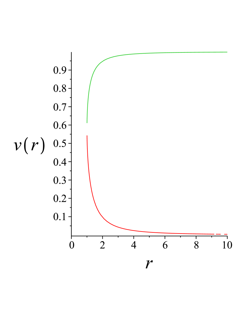
Figure 1: Plot of $v_{z}(z)$ for the spherically symmetric case given by Eqn.(31) with $z_{h}=1$. There are two physical branches; neither is valid for $z<z_{h}$. The third branch is superluminal.

This cubic equation for $v_{z}$ has two physical branches, one subsonic and the other supersonic; the third branch is superluminal. The physical branches are plotted in Fig. 1. In the subsonic branch, as $z\to\infty$, $v_{z}\to 0$ which is consistent with the identification (26). At the horizon the derivatives blow up:

$$-\frac{dv_{z}}{dz}=\frac{\Phi_{S}}{\mathcal{T}_{\infty}^{3}}\frac{2}{3z^{3}(1-3v_{z}^{2})}\to\infty{\rm\ at\ }\ z=z_{h}.$$ (32)

As a result, quantities like the Hawking temperature blow up and more importantly the hydrodynamic description breaks down. The pathology can possibly be cured by introducing a viscosity [16], i.e.​ by going to higher orders of the hydrodynamic derivative expansion.

2.1.2 Solution in more general geometries

To obtain solutions of first order hydrodynamics that are valid globally, we can choose a more general $R(z)$ such that

• the spacetime is asymptotically flat, $R(z)\sim|z|$ for $z\to\pm\infty$

• the maximum value of the RHS of (28) is $\frac{2}{3\sqrt{3}}$, the same as the maximum possible value of the LHS. This condition implies that the minimum value attained by $R(z)$ is

$$R_{\rm min}=\left(\frac{3\sqrt{3}}{2}\frac{\Phi_{S}}{\mathcal{T}_{\infty}^{3}}\right)^{1/2}.$$ (33)

Then we can construct a smooth solution that changes over from subsonic to supersonic or vice-versa every time $R(z)$ attains the above minimum value. For a generic velocity profile, the derivatives at the horizon do not blow up because the divergence of $\frac{dv_{z}}{dR(z)}$ at the horizon is canceled by the fact that

$$\frac{dR(z)}{dz}=-R(z)\frac{1-3v_{z}^{2}}{2v_{z}(1-v_{z}^{2})}\frac{dv_{z}}{dz}=0{\rm\ at}\ z=z_{h}.$$ (34)

The simplest example is the wormhole geometry given by

$$R(z)=\sqrt{z^{2}+z_{0}^{2}}\,.$$ (35)

There are two asymptotically flat sheets as $z\to\pm\infty$ which are connected by a throat at $z=0$, where $R(z)=R_{\rm min}=z_{0}$. From (33) we get the condition $\frac{\Phi_{S}}{\mathcal{T}_{\infty}^{3}}=\frac{2z_{0}^{2}}{3\sqrt{3}}$, and (28) then gives

$$v_{z}(1-v_{z}^{2})=\frac{\Phi_{S}}{\mathcal{T}_{\infty}^{3}}\frac{1}{R(z)^{2}}=\frac{2}{3\sqrt{3}}\frac{z_{0}^{2}}{z^{2}+z_{0}^{2}}\,.$$ (36)

The cubic equation for can be solved for $v_{z}$. Again there are two physical (subluminal) branches. One of them smoothly increases from $v_{z}=0$ to $v_{z}=1$ for $z\in(-\infty,\infty)$ while the other one smoothly decreases. Both solutions have acoustic horizons at $z=0$. A plot of the solutions is given in Fig. 2.

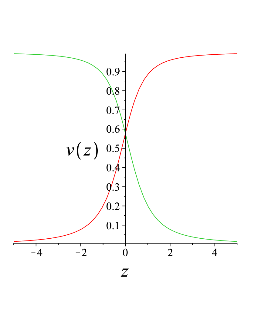
Figure 2: Plot of $v_{z}(z)$ for the wormhole geometry (35) with $z_{0}=1$. There are two physical branches, making a subsonic to supersonic (supersonic to subsonic) transition at the acoustic horizon at $z=0$.

The velocity and its derivatives remain finite near the horizon, as seen from the near-horizon expansion of the increasing solution:

$$v_{z}=\frac{1}{\sqrt{3}}+\frac{\sqrt{2}}{3}\frac{z}{z_{0}}$$ (37)

and the acoustic Hawking temperature is

$$T_{H}=\frac{3}{4\pi}\left|\frac{dv_{z}}{dz}\right|_{z=0}=\frac{1}{2\sqrt{2}\pi z_{0}}\,.$$ (38)

An obvious problem with this solution is that it reaches the speed of light asymptotically on one of the sheets.

To fix this problem, we can choose, for example

$$R(z)=(z^{4}-2z^{2}z_{0}^{2}+z_{0}^{4}+R_{\rm min}^{4})^{\frac{1}{4}}$$ (39)

which is smooth for $R_{\rm min}>0$ and has minima at $z=\pm z_{0}$ where $R(z)=R_{\rm min}$. (33) sets $\frac{\Phi_{S}}{\mathcal{T}_{\infty}^{3}}=\frac{2R_{\rm min}^{2}}{3\sqrt{3}}$. This is geometry where two asymptotically flat regions separated by a wormhole with two throats. For the velocity profile, we have

$$v_{z}(1-v_{z}^{2})=\frac{\Phi_{S}}{\mathcal{T}_{\infty}^{3}}\frac{1}{R(z)^{2}}=\frac{2}{3\sqrt{3}}\frac{R_{\rm min}^{2}}{\sqrt{z^{4}-z^{2}z_{0}^{2}+z_{0}^{4}+R_{\rm min}^{4}}}\,.$$ (40)

Now we can find a solution that crosses over from subsonic to supersonic and back to subsonic at the horizons and remains subluminal for all $z$, as shown in Fig. 3.

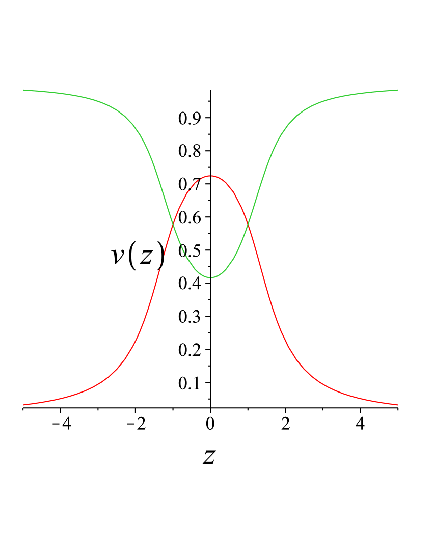
Figure 3: Plot of $v_{z}(z)$ for the geometry with two throats given by Eqn.(39) with $z_{0}=1$, $R_{\rm min}=1$. There are two horizons located at $z_{h}=\pm z_{0}$. The red branch remains subluminal for all $z$.

2.1.3 Nozzle geometry

We can also choose the spatial section of the metric to be asymptotically cylindrical with $R(z)\to$ constant at $z\to\pm\infty$. For variety we consider geometries with a toroidal cross-section

$$ds^{2}=-dt^{2}+dz^{2}+R(z)^{2}(d\theta_{1}^{2}+d\theta_{2}^{2}).$$ (41)

The form of the acoustic metric (23) remains very similar with the replacement of $d\Omega_{2}^{2}$ by $d\theta_{1}^{2}+d\theta_{2}^{2}$. The acoustic Hawking temperature is still given by (25). As an example, we can take the following profile for $v(z)$ and then solve (28) for $R(z)$:

$$v_{z} = v_{\rm min}+(v_{\rm max}-v_{\rm min})\,\text{sech}\left(\frac{z}{z_{0}}\right)\,.$$ (42)

The $v_{\rm min}$ term ensures that $R(z)\to$ constant and remains finite for large $|z|$. The profiles of $v(z)$ and $R(z)$ are shown in Fig. 4.

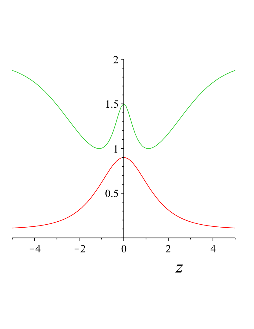
Figure 4: Velocity profile (in red) for the nozzle geometry given by Eqn.(42) with $v_{\rm min}=0.1$, $v_{\rm max}=0.9$, $z_{0}=1$ and the corresponding $R(z)/R_{\rm min}$ (in green). The minima in $R(z)$ at $z=\pm z_{0}$ correspond to $v=c_{s}$.

There are two horizons located at

$$z_{\pm}=\pm z_{0}\cosh^{-1}\frac{v_{\rm max}-v_{\rm min}}{c_{s}-v_{\rm min}}\,.$$ (43)

Assuming $v_{z}>0$, the fluid passes the speed of sound at the left horizon $z_{-}$ and again returns to subsonic speeds as it crosses the right horizon $z_{+}$.

2.2 Sound waves

In this subsection we examine the behavior of sound waves around the background flows described in the previous subsections. Sound waves are fluctuations of the velocity potential $\phi$ which satisfy a massless Klein-Gordon equation in the background acoustic metric (2.1). We will consider background flows on a simple wormhole geometry - more complicated wormholes or nozzle geometries can be treated along similar lines.

Near the acoustic horizon (chosen at $z=0$), the metric is similar to the usual Schwarzschild metric, so we expect a large blueshift effect for outgoing modes. To display this, it is sufficient to consider modes in the $s$-wave. Let us first rewrite the metric in terms of null coordinates $u,v$ as follows

$$d\tilde{s}^{2}=\sqrt{3}\mathcal{T}^{2}(z)\left\{-(1-\frac{2}{3}\gamma^{2})dudv+R^{2}(z)(d\theta^{2}+\sin^{2}\theta d\phi^{2})\right\},$$ (44)

where

$$du=d\tau-\frac{dz}{\sqrt{3}(1-\frac{2}{3}\gamma^{2})}=dt+\frac{\frac{2}{3}\gamma^{2}v\,dz}{1-\frac{2}{3}\gamma^{2}}-\frac{dz}{\sqrt{3}(1-\frac{2}{3}\gamma^{2})}=dt-\frac{dz}{v_{+}(z)}$$

$$dv=d\tau+\frac{dz}{\sqrt{3}(1-\frac{2}{3}\gamma^{2})}=dt+\frac{\frac{2}{3}\gamma^{2}v\,dz}{1-\frac{2}{3}\gamma^{2}}+\frac{dz}{\sqrt{3}(1-\frac{2}{3}\gamma^{2})}=dt-\frac{dz}{v_{-}(z)}\,.$$ (45)

Here $v_{\pm}(z)=\frac{v(z)\pm c_{s}}{1\pm v(z)c_{s}}$ is the relativistic sum of the local fluid velocity and the velocity of sound $c_{s}=1/\sqrt{3}$. Then close to the acoustic horizon $R(z)\rightarrow R(0)$ is finite, and the $s$-wave solutions of the Klein-Gordon equation are approximately

$$\psi_{+}\sim e^{-i\omega u}\hskip 28.45274pt\psi_{-}\sim e^{-i\omega v}\,.$$ (46)

In the asymptotic region, where the velocity becomes constant, we obtain the usual spherical Bessel functions. To analyze the near-horizon behavior, we can expand the velocity field near the horizon as $v(z)\approx c_{s}+\frac{2}{3}\kappa z+\ldots$, where $\kappa=\frac{3}{2}\left|\frac{dv}{dz}\right|_{z_{h}}$ is the surface gravity at the horizon. Using this in (46), we find

$$\psi_{+} \sim e^{-i\omega\left[t-\frac{2z}{\sqrt{3}}+O(z^{2})\right]}$$ (47)

$$\psi_{-} \sim e^{-i\omega\left[t-\frac{1}{\kappa}\ln\left|z\right|+\frac{z}{\sqrt{3}}+O(z^{2})\right]}$$ (48)

The $\psi_{+}$ mode is continuous at the horizon and is right moving with a velocity $\frac{\sqrt{3}}{2}$, which is the relativistic sum of $\frac{1}{\sqrt{3}}$ with itself. The $\psi_{-}$ mode has rapid oscillations near the horizon:

$$z\lesssim 0\ : \psi_{-}\sim e^{-i\omega\left[t-\frac{1}{\kappa}\ln(-z)\right]}\hskip 14.22636pt\mbox{(left-moving)}$$

$$z\gtrsim 0\ : \psi_{-}\sim e^{-i\omega\left[t-\frac{1}{\kappa}\ln(z)\right]}\hskip 14.22636pt\mbox{\rm(right-moving)}$$

indicating that inside the horizon, both modes are right-moving.

To extend these modes away from the horizon, we employ an eikonal approximation. We decompose the sonic fluctuation into a rapidly varying phase or “eikonal” (here $\lambda\gg 1$) times a slowly varying envelope

$$\psi(x^{\mu})=A(x^{\mu})e^{-i\lambda S(x^{\mu})}$$ (49)

and plug it into the wave equation $\partial_{\mu}\left[\sqrt{-G}G^{\mu\nu}\partial_{\nu}\right]\psi=0$ with the acoustic metric (21) written out in the original $t$-$z$ coordinates

$$d\tilde{s}^{2}=\mathcal{T}^{2}\left\{-(1-\frac{2}{3}\gamma^{2})dt^{2}-\frac{4}{3}\gamma^{2}v_{z}dtdz+(1+\frac{2}{3}\gamma^{2}v_{z}^{2})dz^{2}+R(z)^{2}(d\theta^{2}+\sin^{2}\theta d\phi^{2})\right\}\,.$$ (50)

We then get a sequence of differential equations for $S(x^{\mu})$ and $A(x^{\mu})$ by expanding the wave equation order by order in $\lambda$:

$$O(\lambda^{2}) : \partial_{\mu}S(x^{\alpha})\partial^{\mu}S(x^{\alpha})=0$$ (51)

$$O(\lambda) : 2\partial_{\mu}S(x^{\alpha})\partial^{\mu}A(x^{\alpha})+A(x^{\alpha})\nabla^{2}S(x^{\alpha})=0$$

$$\vdots$$

The leading equation (51) can be used to solve for $S(x^{\alpha})$. Let us consider $s$-wave solutions independent of $\theta,\phi$. With the ansatz

$$\lambda S(x^{\alpha})=\omega t-f(z)$$ (53)

we can solve for the phase,

$$\lambda S_{\pm}(x^{\alpha})=\omega t+\omega\int dz\,\frac{\frac{2}{3}\gamma^{2}v\mp\frac{1}{\sqrt{3}}}{1-\frac{2}{3}\gamma^{2}}=\omega t-\omega\int dz\,\frac{1\pm\frac{v}{\sqrt{3}}}{v\pm\frac{1}{\sqrt{3}}}$$ (54)

The momenta of the wavepackets are given by derivatives of the eikonal  $p_{\mu}\equiv-\partial_{\mu}[\lambda S(x^{\alpha})]$ giving

$$p_{t} = \omega$$

$$p_{z} = \omega\,\frac{1\pm vc_{s}}{v\pm c_{s}}=\frac{\omega}{v_{\pm}}\,,$$ (55)

where $v_{\pm}$ has been defined above. The upper and the lower signs would normally correspond to right- and left-moving sound modes. However, if the fluid (assumed to be right moving) has a velocity greater than the speed of sound, then both the modes become right-moving. Using the ansatz $A(x^{\alpha})=A(z)$ in the subleading equation (2.2), a full solution is obtained:

$$\psi_{\pm}=\frac{A_{0}}{\mathcal{T}R(z)}e^{-i\omega\left[t-\int\frac{dz}{v\pm(z)}\right]}$$ (56)

3 Gravity dual of acoustic solution

The fluid-gravity correspondence [3, 4, 5, 6, 7, 21, 22] provides a correspondence between solutions of certain fluids with classical solutions of suitable Einstein-Maxwell equations in a $4+1$ dimensional spacetime with a negative cosmological constant. In our case the fluid is a conformal fluid with a global U$(1)$ charge and the higher dimensional bulk theory is given by the five-dimensional action

$$S=\frac{1}{16\pi G}\int d^{5}x~{}{\sqrt{-g}}\left[R+12-F_{AB}F^{AB}-\frac{4\kappa}{3}\epsilon^{EABCD}A_{E}F_{AB}F_{CD}\right]$$ (57)

where $G$ is the five dimensional Newton constant, the indices $A,B$ run from 0 to 4, $A_{B}$ is a U$(1)$ gauge field, and we have chosen units in which the cosmological constant is $\Lambda=-6$. The above action is a consistent truncation of IIB supergravity for $\kappa=1/(2\sqrt{3})$. We will, however, allow arbitrary values of $\kappa$.

A uniform charged black brane solution of this action is given in a boosted reference frame by

$$ds^{2} = -2u_{\mu}dx^{\mu}dr-r^{2}V(r,m,{\tilde{q}})u_{\mu}u_{\nu}dx^{\mu}dx^{\nu}+r^{2}P_{\mu\nu}dx^{\mu}dx^{\nu}$$

$$A = \frac{{\sqrt{3}}{\tilde{q}}}{2r^{2}}u_{\mu}dx^{\mu}$$ (58)

where $u_{\mu}$ are constant 4-velocities (the indices $\mu,\nu=0\cdots 3$) and $P_{\mu\nu}=\eta_{\mu\nu}+u_{\mu}u_{\nu}$ is the spatial projection operator. The function $V(r,m,{\tilde{q}})$ is given by

$$V(r,m,{\tilde{q}})=1-\frac{m}{r^{4}}+\frac{{\tilde{q}}^{2}}{r^{6}}$$ (59)

where $m$ and ${\tilde{q}}$ are parameters of the solution and we are using the notation of [22].

This solution is dual to a charged fluid in equilibrium living on the flat boundary of the five-dimensional spacetime. The fluid is strongly-coupled $\mathcal{N}=4$ SU$(N)$ Yang-Mills theory, viewed in a boosted frame with coordinates $x^{\mu}$. The temperature $T$, charge density $q$, energy density $\epsilon$ and entropy density $s$ of the fluid are given by [22]

$$T=\frac{R_{+}}{2\pi}\left(2-\frac{{\tilde{q}}^{2}}{R_{+}^{6}}\right),\hskip 14.22636ptq=\sqrt{3}\alpha{\tilde{q}},\hskip 14.22636pt\epsilon=3\alpha m,\hskip 14.22636pts=4\pi\alpha R_{+}^{3},\hskip 14.22636pt\alpha\equiv\frac{1}{16\pi G}$$ (60)

where $R_{+}$ denotes the radius of the outer horizon, i.e. the largest root of the equation $V(r,m,{\tilde{q}})=0$. The energy momentum tensor $T_{\mu\nu}$ and the charge current $J_{\mu}$ of the fluid are given by

$$T_{\mu\nu}=\frac{\epsilon}{3}(\eta_{\mu\nu}+4u_{\mu}u_{\nu})~{}~{}~{}~{}~{}~{}~{}~{}~{}~{}~{}~{}~{}~{}~{}J_{\mu}=qu_{\mu}$$ (61)

The expressions (60) and (61) involve the bulk parameter $G$. In our units, $G$ is related to the rank of the gauge group of the boundary theory by

$$G=\frac{\pi}{2N^{2}},\hskip 28.45274pt\alpha=\frac{1}{16\pi G}=\frac{N^{2}}{8\pi^{2}}.$$ (62)

With the substitutions in (60), the equation of state $\epsilon(s,q)$ becomes identical to the condition $V(R_{+}(s),m(\epsilon),{\tilde{q}}(q))=0$. The equation of state for a charged conformal fluid with a gravity dual is thus

$$1-\frac{\epsilon}{3\alpha R_{+}^{4}}+\frac{q^{2}}{3\alpha^{2}R_{+}^{6}}=0,{\rm{\ with\ }}R_{+}=\left(\frac{s}{4\pi\alpha}\right)^{\frac{1}{3}}$$ (63)

$$\Rightarrow \epsilon(s,q)=3\alpha\left(\frac{s}{4\pi\alpha}\right)^{\frac{4}{3}}+\frac{q^{2}}{\alpha}\left(\frac{4\pi\alpha}{s}\right)^{\frac{2}{3}}$$ (64)

The temperature and chemical potential can be obtained by taking derivatives of $\epsilon(s,q)$ using (5):

$$T = \frac{1}{\pi}\left(\frac{s}{4\pi\alpha}\right)^{1/3}\left(1-\frac{8\pi^{2}q^{2}}{3s^{2}}\right)$$

$$\mu = 2\left(\frac{q}{\alpha}\right)\left(\frac{4\pi\alpha}{s}\right)^{2/3}$$ (65)

This temperature reproduces the value quoted in (60). In the uncharged limit $R_{+}=\pi T$, and one can fix the value of $c$ defined in (7) by comparing it with (63) and requiring that $\mathcal{T}=T$ for uncharged fluids; this gives $c=\alpha\pi^{4}$ and hence

$$\epsilon_{\mu=0}=3\alpha(\pi T)^{4}\,,~{}~{}~{}~{}s_{\mu=0}=4\pi\alpha(\pi T)^{3}\,.$$ (66)

For charged fluids at finite $\mu$ there is a zero-temperature limit, reached when $R_{+}=\mu/(2\sqrt{6})$ and $\mathcal{T}=\mu/(192^{\frac{1}{4}}\pi)$. In this limit,

$$q_{T=0}=\frac{\alpha}{48}\mu^{3}\,,~{}~{}~{}~{}\epsilon_{T=0}=\frac{\alpha}{64}\mu^{4}\,,~{}~{}~{}~{}s_{T=0}=\frac{\pi\alpha}{12\sqrt{6}}\mu^{3}\,.$$ (67)

As discussed in Section 2 we restrict our attention to isentropic flows. For such flows $q/\mathcal{T}^{3}$ is constant and since $\epsilon=3\alpha\pi^{4}\mathcal{T}^{4}$, it follows from the equation of state (63) that $\mathcal{T}/R_{+}$ is a constant, and therefore that for such flows the entropy per unit charge $s/q$ is constant. The first equation in (65) shows that by choosing

$$1-\frac{8\pi^{2}}{3}\left(\frac{s}{q}\right)^{2}\ll 1$$ (68)

we can keep the temperature $T\ll R_{+}$ everywhere and at all times.

The gravity dual of a general fluid motion is then constructed in a derivative expansion as follows. First, we replace the parameters of the solution by functions of the boundary coordinates $x^{\mu}$, $u^{\mu}\rightarrow u^{\mu}(x),m\rightarrow m(x),{\tilde{q}}\rightarrow{\tilde{q}}(x)$ which respectively represent the velocity field, energy density field and the charge density field of the fluid. We also replace the flat boundary metric $\eta_{\mu\nu}$ with a curved metric $g_{\mu\nu}(x)$. With these replacements, (58) is no longer a solution of the bulk equations of motion. Second we need to add correction terms to the metric and the gauge field so that the full metric and the gauge field now solve the equations of motion. This second step is of course impossible to perform in an exact fashion. However, these corrections can be calculated systematically in a derivative expansion, provided that the derivatives of $u^{\mu}(x),\ m(x),\ {\tilde{q}}(x)$ with respect to $x^{\nu}$ are small compared to the outer horizon radius $R_{+}$. To lowest nontrivial order in the derivative expansion, the modified metric and gauge fields are

$$ds^{2} = -2u_{\mu}dx^{\mu}dr-r^{2}V(r,m,{\tilde{q}})u_{\mu}u_{\nu}dx^{\mu}dx^{\nu}+r^{2}P_{\mu\nu}dx^{\mu}dx^{\nu}$$ (69)

$$+ \frac{2}{3}r(\nabla_{\alpha}u^{\alpha})u_{\mu}u_{\nu}dx^{\mu}dx^{\nu}+\frac{2r^{2}}{R_{+}}\sigma_{\mu\nu}F_{2}(\rho,M)dx^{\mu}dx^{\nu}$$

$$- 2ru_{\mu}u^{\alpha}(\nabla_{\alpha}u_{\nu})dx^{\mu}dx^{\nu}$$

$$- 2u_{\mu}\left(\frac{\sqrt{3}\kappa{\tilde{q}}^{3}}{mr^{4}}l_{\nu}+\frac{6r^{2}}{R_{+}^{7}}(P^{\lambda}_{\nu}\partial_{\lambda}{\tilde{q}}+3(u^{\lambda}\nabla_{\lambda}u_{\nu}){\tilde{q}})F_{1}(\rho,M)\right)dx^{\mu}dx^{\nu},$$

$$A=\left[\frac{\sqrt{3}{\tilde{q}}}{2r^{2}}u_{\mu}+\frac{3\kappa{\tilde{q}}^{2}}{2mr^{2}}l_{\mu}-\frac{\sqrt{3}r^{5}}{2R_{+}^{8}}(P^{\lambda}_{\mu}\partial_{\lambda}{\tilde{q}}+3(u^{\lambda}\nabla_{\lambda}u_{\mu}){\tilde{q}})\right]dx^{\mu}$$ (70)

where we have defined the quantities

$$M=\frac{m}{R_{+}^{4}}~{}~{}~{}~{}~{}~{}~{}~{}Q=\frac{{\tilde{q}}}{R_{+}^{3}}~{}~{}~{}~{}~{}~{}~{}\rho=\frac{r}{R_{+}}\,.$$ (71)

$\nabla_{\mu}$ is a covariant derivative with boundary metric $g_{\mu\nu}$, and

$$l_{\mu}=g_{\mu\gamma}\epsilon^{\nu\alpha\beta\gamma}u_{\nu}\nabla_{\alpha}u_{\beta}\,,~{}~{}~{}~{}~{}~{}~{}~{}\sigma_{\mu\nu}=\frac{1}{2}P^{\mu\alpha}P^{\nu\beta}\left(\nabla_{\alpha}u_{\beta}+\nabla_{\beta}u_{\alpha}\right)-\frac{1}{3}P^{\mu\nu}(\nabla_{\alpha}u^{\alpha})\,.$$ (72)

The functions $F_{1}(\rho,M,Q)$ and $F_{2}(\rho,M)$ are defined as

$$F_{1}(\rho,M,Q) = \frac{1}{3}\left(1-\frac{M}{\rho^{4}}+\frac{Q^{2}}{\rho^{6}}\right)\int^{\infty}_{\rho}dp\frac{1}{(1-\frac{M}{\rho^{4}}+\frac{Q^{2}}{\rho^{6}})^{2}}\left(\frac{1}{p^{8}}-\frac{3}{4p^{7}}(1+\frac{1}{M})\right),$$ (73)

$$F_{2}(\rho,M) = \int_{\rho}^{\infty}dp\frac{p(p^{2}+p+1)}{(p+1)(p^{4}+p^{2}-M+1)}$$ (74)

Note that in the above expressions $m,{\tilde{q}},R_{+},M,Q,\rho$ are also functions of the boundary coordinates $x^{\mu}$ since $m$ and ${\tilde{q}}$ are functions of $x^{\mu}$.

This is a solution of the bulk equations of motion, provided that $m(x)$, ${\tilde{q}}(x)$ and $u_{\mu}(x)$ are such that the energy momentum tensor and current

$$T_{\mu\nu}=\frac{m(x)}{16\pi G}(g_{\mu\nu}(x)+4u_{\mu}(x)u_{\nu}(x))~{}~{}~{}~{}~{}J_{\mu}=\frac{\sqrt{3}{\tilde{q}}(x)}{16\pi G}u_{\mu}(x)$$ (75)

are covariantly conserved,

$$\nabla_{\mu}T^{\mu\nu}=\nabla_{\mu}J^{\mu}=0$$ (76)

Thus every solution of fluid dynamics leads to a bulk solution.

3.1 Gravity duals of dumb holes

We now apply the results of the preceding subsection to construct gravitational duals of the fluid flows with acoustic horizons that were studied in Section 2. These flows are special in several ways: first, the background spacetime metric of the fluid is of the form (23) or (41) where the only inhomogeneity is in the $z$ direction. Second, both the background flow and the sound wave fluctuations have vanishing vorticity. Third, the background flows as well perturbations around them are isentropic.

It follows from the isentropic condition that the quantities $M$ and $Q$ are constants. As argued above (see discussion following equation (15)), for isentropic flows there is just one length scale, and all quantities are related to this length scale by dimensional analysis. In particular, the dimensionless quantities $M$ and $Q$ must be constant. In addition, the inhomogeneous parts of all quantities which appear in the bulk metric and the gauge field are determined in terms of a single scalar field $\phi(x)$.

As discussed in the introduction, in order for the acoustic Hawking radiation to be detectable we need to consider fluids which have a very small ambient temperature. This means that the constant quantities $Q$ and $M$ need to be close to their extremal values, $Q\approx{\sqrt{2}}$ and therefore $M\approx 3$. While the various quantities like $\epsilon(x),q(x)$ can change by ${\cal O}(1)$ amounts (only their derivatives are small), the isentropic condition ensures that if the fluid temperature is initially small it will remain small (see the discussion in Section 2 above).

To construct the background fluid flow, we simply need to insert the velocity potential $\phi_{0}$ for the solutions of Section 2 into the general metric and gauge field in (69) and (70). The conditions of vanishing vorticity and isentropic flow simplify these general expressions somewhat. The most drastic simplification appears in the expression for the gauge field, equation (70). In fact the first order corrections (in the derivative expansion) to the gauge field vanish for isentropic gradient flows. To see this we note first that $\nabla_{\alpha}u_{\beta}$ can be replaced by $\partial_{\alpha}u_{\beta}$ in the expression $l_{\mu}$ of (72). Then using $\mathcal{T}u_{\mu}=\partial_{\mu}\phi$ we get

$$l_{\mu}=g_{\mu\gamma}\epsilon^{\nu\alpha\beta\gamma}\frac{\partial_{\nu}\phi}{\mathcal{T}}[-\frac{1}{\mathcal{T}^{2}}\partial_{\alpha}\mathcal{T}\partial_{\beta}\phi+\frac{1}{\mathcal{T}}\partial_{\alpha}\partial_{\beta}\phi]=0$$ (77)

due to antisymmetry of the epsilon symbol. The third term on the RHS of (70) also vanishes, as can be seen by applying the isentropic condition $q/\mathcal{T}^{3}=$constant and the relations (14) and (15) to the expression

$$P^{\lambda}_{\mu}\nabla_{\lambda}{\tilde{q}}+3(u^{\lambda}\nabla_{\lambda}u_{\mu}){\tilde{q}} = 3a\mathcal{T}\left[\mathcal{T}\partial_{\mu}\mathcal{T}+\mathcal{T}u^{\lambda}\nabla_{\lambda}(\mathcal{T}u_{\mu})\right]$$ (78)

$$= 3a\mathcal{T}\left[-\frac{1}{2}\partial_{\mu}(\partial_{\alpha}\phi\partial^{\alpha}\phi)+\partial^{\lambda}\phi\nabla_{\lambda}\partial_{\mu}\phi\right]=0$$

Thus, to first order in the derivative expansion, the bulk gauge field is given by the first term of the right hand side of (70), which is just the term which would have resulted from a simple boost of the original black brane solution. In our case the charge density and the 4-velocity appearing in (70) are functions of $z$, as determined by the fluid flow on the boundary. So there is a nonzero electric field component along the $z$ direction, given by

$$F_{0z}=-\frac{\sqrt{3}{\tilde{q}}_{\infty}}{r^{2}}v_{z}\partial_{z}v_{z}$$ (79)

where we have used (29) to express $q(z)$ in terms of the velocity $v_{z}$.

The expression for the bulk metric simplifies as well. In the fourth line of (69), the first term is proportional to $l_{\mu}$ which vanishes for our flows. The second term is proportional to $H_{\mu}$ defined in (78) and vanishes as shown above.

In the derivative expansion, the relationship between the boundary and the bulk becomes essentially local. The bulk solution can in fact be constructed approximately by patching together tube geometries obtained by extending the boundary data in a given region of the boundary to the bulk using the radial equations of motion. Consequently we expect that the acoustic horizon of the fluid flow on the boundary extends trivially into the bulk. We will explicitly verify this in the next subsection.

However, this tubewise approximation breaks down in regions where the local geometry is exactly extremal. This is apparent in the results of [21] and [22]. Furthermore, recent work on perturbations around extremal black holes shows that the relevant low energy expansion is different from the naive derivative expansion [24]. Our results hold close to extremality, but not exactly at extremality.

3.2 Gravity duals of phonons

The gravity duals of phonons in the fluid are quasinormal modes of metric and gauge field perturbations. Once again, construction of these modes is trivial. We need to write

$$\phi(x^{\mu})=\phi_{0}(x^{\mu})+\beta\delta\phi(x^{\mu}),$$ (80)

compute $\mathcal{T}(x)$ and hence $m(x),q(x),u_{\mu}(x)$ in terms of $\delta\phi$, substitute into (69) and (70), and consider the terms which are linear in $\beta$. By construction, these modes satisfy ingoing boundary conditions at the bulk horizon.

The fluctuations of the gauge field $A_{\mu}$ obtained by this procedure have a particularly simple form

$$\delta A_{\mu}=-\beta\frac{\sqrt{3}a}{2r^{2}}[(\partial_{\beta}\phi_{0})(\partial^{\beta}\phi_{0})\delta^{\alpha}_{\mu}+(\partial_{\mu}\phi_{0})(\partial^{\alpha}\phi_{0})]\partial_{\alpha}(\delta\phi)$$ (81)

For the background flows considered in Section 2, we have found solutions to the wave equation (2) for $\delta\phi$ in the region close to the acoustic horizon. Upon inserting these solutions into (81), we see that the fluctuations $\delta A_{\mu}$ have a characteristic behavior near the acoustic horizon, viz. ingoing waves are smooth while outgoing waves have rapid fluctuations. This is the precise sense in which the fluctuations perceive the acoustic horizon, which has now extended into the bulk. From the nature of the solution that the extension of the acoustic horizon into the bulk is rather trivial - i.e. the horizon perceived by these modes is at the same value of $z$ as the acoustic horizon on the boundary, and for all values of $r$.

The fluctuations for the components of the metric can be similarly worked out and also see a horizon structure at the same value of $z$. We therefore conclude that there are certain quasinormal modes of the bulk metric and the gauge field which perceive a horizon. If these bulk modes are quantized, one should find a thermal bath of such modes characterized by the temperature of the acoustic horizon on the boundary.

4 Regime of validity

It is important to check that the fluid flow described above is consistent with the standard conditions for validity of hydrodynamics. Roughly speaking, hydrodynamics is valid when the gradients of velocities, temperature and charge densities are small compared to the inverse mean free path $l_{m}$. For charged conformal fluids considered above, there are two scales - the temperature $T$ and the chemical potential $\mu\equiv\nu T$, so that $l_{m}\sim f(\nu)/T$. The function $f(\nu)$ is of order one for generic values of $\nu$, but there is an upper bound on $\nu$, $\nu_{c}$ where $f(\nu)$ has a simple zero. It is possible to take the limit of $\nu\rightarrow\nu_{c}$ simultaneously with $T\rightarrow 0$ such that $l_{m}$ is finite - the dual of this is in fact the extremal black hole. For the flow described in the previous section, in this limit we have

$$\left|\frac{dv_{z}(z)}{dz}\right| \ll \frac{1}{l_{m}}$$

$$\left|\frac{1}{\mathcal{T}}\frac{d\mathcal{T}(z)}{dz}\right| \ll \frac{1}{l_{m}}$$ (82)

In particular, since the acoustic Hawking temperature $T_{H}$ is $\frac{3}{4\pi}\left|\frac{dv_{z}}{dz}\right|_{z_{\mp}}$, this implies that

$$T_{H}\ll\frac{1}{l_{m}}$$ (83)

For observable acoustic Hawking radiation, the Hawking temperature should be higher than the fluid temperature. So we require

$$T\lesssim T_{H}$$ (84)

Furthermore, the frequency of the sound waves should also be small compared to the basic scale, $\omega\ll 1/l_{m}$. However, the finite Hawking temperature is going to introduce an upper bound on the allowed wavelengths, due to periodicity in Euclidean time; thus $\omega>T_{H}$. Thus we need

$$T\lesssim T_{H}<\omega\ll\frac{1}{l_{m}}$$ (85)

For fluids with no conserved charge, there is only one energy scale, namely, the temperature $T$; thus $1/l_{m}\sim T$ and (84) cannot be satisfied. Although the solution is otherwise valid, the Hawking radiation, at a temperature much lower than the ambient temperature, is not going to be observable. For fluids with a conserved charge the condition (84) does not pose a problem because now we have two length scales, the temperature $T$ and the chemical potential $\mu$. For fluids very close to zero temperature, the mean free path will be governed only by $\mu$. We can thus have

$$0\approx T\lesssim T_{H}<\omega\ll\frac{1}{l_{m}}\approx\mathcal{T}\approx\mu$$ (86)

The ability to construct a gravity dual using a derivative expansion imposes further conditions. In the presence of a nonconstant $R(z)$, the validity of the derivative expansion of the solutions of the bulk equations of motion requires that the curvature invariants and all invariants constructed out of the derivatives of curvature be small. An example of such an invariant is $g^{\mu\nu}\nabla_{\mu}\mathcal{R}\nabla_{\nu}\mathcal{R}$, where $\mathcal{R}$ is the Ricci scalar and we require for this example

$$(g^{\mu\nu}\,\nabla_{\mu}\,\mathcal{R}\nabla_{\nu}\,\mathcal{R})^{\frac{1}{6}}\ll\frac{1}{l_{m}}\,.$$ (87)

We get additional conditions if some of the boundary directions are compactified as in the nozzle geometry of Section (2.1.3). If one boundary direction of a $AdS\times S$ geometry is made compact with a radius $R(z)$, the dual is an $AdS$ soliton [25] which caps off the geometry at a value of the radial coordinate $r=1/(2R)$. For a black brane geometry, compactification of a boundary direction would lead to a similar modification of the usual black brane geometry. However if $R(z)\gg 1/(2R_{+})$, where $R_{+}$ is the location of the black brane horizon, the place where the bulk geometry would cap off is far inside the black brane horizon. In this situation we can continue to use the standard black brane geometry with a compact longitudinal direction. We will therefore require that for all $z$,

$$R(z)\gg 1/R_{+}$$ (88)

for the solution of Section (2.1.3). Finally we require for the nozzle solution that $R(z)$ be finite for large $z$. The geometry is then asymptotically $\mathbb{R}\times{T}^{2}$ and has an AdS dual.

4.1 Validity of our solutions

Finally, we determine the range of parameters for which our approximations are valid, for the specific flows studied in Section 2. Let us first discuss the wormhole solution of equations (39) and (40). The solution has four parameters, $\mathcal{T}_{\infty}$, $q_{\infty}$, $z_{0}$ and $R_{\rm min}$. $\Phi_{S}$ is fixed by (33) once $R_{\rm min}$ is chosen. Since $v<1$, $\gamma$ remains finite for all $z$. $\mathcal{T}=\frac{\mathcal{T}_{\infty}}{\gamma}>0$ and we can have a valid derivative expansion w.r.t. $\mathcal{T}_{\infty}$. In order that the curvatures are small, we require $R_{\rm min}\gg 1/\mathcal{T}_{\infty}$. The derivatives $\frac{dv_{z}}{dz}$, $\frac{1}{\mathcal{T}}\frac{d\mathcal{T}}{dz}$ and the derivatives of the curvature are all proportional to $\frac{1}{z_{0}}$. Thus we require $\frac{1}{z_{0}}\ll\mathcal{T}_{\infty}$. $q_{\infty}$ can be chosen such that we are always at very low temperatures, following the discussion around equation (68). To summarize, the conditions for our wormhole solution to be valid are:

$$T\to 0,\hskip 14.22636pt\frac{1}{z_{0}}<\omega\ll\mathcal{T}_{\infty}\,,\hskip 14.22636pt\frac{1}{R_{\rm min}}\ll\mathcal{T}_{\infty}.$$ (89)

For the nozzle solution described by (42), the parameters are $z_{0}$, $v_{\rm max}$, $v_{\rm min}$, $\mathcal{T}_{\infty}$, $q_{\infty}$ and $\Phi_{S}$. As in the previous case, all derivatives in the solution are proportional to $\frac{1}{z_{0}}$. We need $v_{\rm max}<1$ for the derivative expansion to be valid (so that $\gamma$ remains finite and $\mathcal{T}$ remains non-zero) and we obtain the same conditions as in (89). The condition (88) is same as the requirement that the background curvature remains small: $R_{\rm min}\gg 1/\mathcal{T}_{\infty}$. Since $R_{\rm min}$ is given in terms of $\mathcal{T}_{\infty}$ and $\Phi_{S}$ by (33), this implies $\Phi_{S}\gg\mathcal{T}_{\infty}$. Moreover, we need $v_{\rm min}>0$ in order that $R(z)$ be finite at large $z$ – the asymptotic geometry remains $\mathbb{R}\times{T}^{2}$, and we have an asymptotically AdS gravity dual. Summarizing, the conditions for validity of our nozzle solution are:

$$T\to 0,\hskip 14.22636pt\frac{1}{z_{0}}<\omega\ll\mathcal{T}_{\infty}\ll\Phi_{S},\hskip 14.22636pt0<v_{\rm min}<v_{\rm max}<1.$$ (90)

References

- [1] J. M. Maldacena, Adv. Theor. Math. Phys. 2, 231 (1998) [Int. J. Theor. Phys. 38, 1113 (1999)] [arXiv:hep-th/9711200].
- [2] O. Aharony, S. S. Gubser, J. M. Maldacena, H. Ooguri and Y. Oz, Phys. Rept. 323, 183 (2000) [arXiv:hep-th/9905111].
- [3] G. Policastro, D. T. Son and A. O. Starinets, Phys. Rev. Lett. 87, 081601 (2001) [arXiv:hep-th/0104066]; D. T. Son and A. O. Starinets, Ann. Rev. Nucl. Part. Sci. 57, 95 (2007) [arXiv:0704.0240 [hep-th]].
- [4] G. Policastro, D. T. Son and A. O. Starinets, JHEP 0212, 054 (2002) [arXiv:hep-th/0210220].
- [5] S. Bhattacharyya, V. E. Hubeny, S. Minwalla and M. Rangamani, JHEP 0802, 045 (2008) [arXiv:0712.2456 [hep-th]].
- [6] S. Bhattacharyya et al., JHEP 0806, 055 (2008) [arXiv:0803.2526 [hep-th]].
- [7] S. Bhattacharyya, R. Loganayagam, S. Minwalla, S. Nampuri, S. P. Trivedi and S. R. Wadia, JHEP 0902, 018 (2009) [arXiv:0806.0006 [hep-th]].
- [8] W. G. Unruh, Phys. Rev. Lett. 46, 1351 (1981); W. G. Unruh, Phys. Rev. D 51, 2827 (1995).
- [9] T. Jacobson, Phys. Rev. D 44, 1731 (1991); T. Jacobson, Phys. Rev. D 48, 728 (1993) [arXiv:hep-th/9303103].
- [10] M. Visser, arXiv:gr-qc/9311028; M. Visser, Class. Quant. Grav. 15, 1767 (1998) [arXiv:gr-qc/9712010]; M. Visser, arXiv:gr-qc/9901047.
- [11] C. Barcelo, S. Liberati and M. Visser, Class. Quant. Grav. 18, 1137 (2001) [arXiv:gr-qc/0011026]; C. Barcelo, S. Liberati and M. Visser, Int. J. Mod. Phys. A 18, 3735 (2003) [arXiv:gr-qc/0110036].
- [12] N. Bilic, Class. Quant. Grav. 16, 3953-3964 (1999). [gr-qc/9908002].
- [13] S. Basak and P. Majumdar, Class. Quant. Grav. 20, 3907 (2003) [arXiv:gr-qc/0203059].
- [14] For reviews of the field, see M. Visser, C. Barcelo and S. Liberati, Grav. 34, 1719 (2002) [arXiv:gr-qc/0111111]; GRGVA,34,1719;Black Holes,” [http://www.slac.stanford.edu/spires/find/hep/www?irn=5463912] River Edge, USA: World Scientific (2002) 391 p
- [15] M. Visser, Int. J. Mod. Phys. D12, 649-661 (2003). [hep-th/0106111].
- [16] S. Liberati, S. Sonego, M. Visser, Class. Quant. Grav. 17, 2903 (2000). [gr-qc/0003105].
- [17] A. M. Awad and C. V. Johnson, Phys. Rev. D 61, 084025 (2000) [arXiv:hep-th/9910040]; A. M. Awad and C. V. Johnson, Phys. Rev. D 63, 124023 (2001) [arXiv:hep-th/0008211]; A. M. Awad, Class. Quant. Grav. 20, 2827 (2003) [arXiv:hep-th/0209238]; A. M. Awad, Int. J. Mod. Phys. D 18, 405 (2009) [arXiv:0708.3458 [hep-th]].
- [18] S. Bhattacharyya, S. Lahiri, R. Loganayagam and S. Minwalla, JHEP 0809, 054 (2008) [arXiv:0708.1770 [hep-th]].
- [19] S. E. Perez Bergliaffa, K. Hibberd, M. Stone and M. Visser, arXiv:cond-mat/0106255.
- [20] N. Bilic, Class. Quant. Grav. 16, 3953 (1999) [arXiv:gr-qc/9908002].
- [21] J. Erdmenger, M. Haack, M. Kaminski and A. Yarom, JHEP 0901, 055 (2009) [arXiv:0809.2488 [hep-th]].
- [22] N. Banerjee, J. Bhattacharya, S. Bhattacharyya, S. Dutta, R. Loganayagam and P. Surowka, arXiv:0809.2596 [hep-th].
- [23] T. Nishioka, S. Ryu and T. Takayanagi, JHEP 1003, 131 (2010) [arXiv:0911.0962 [hep-th]].
- [24] H. Liu, J. McGreevy and D. Vegh, arXiv:0903.2477 [hep-th]; T. Faulkner, H. Liu, J. McGreevy and D. Vegh, arXiv:0907.2694 [hep-th]; M. Edalati, J. I. Jottar and R. G. Leigh, JHEP 1001, 018 (2010) [arXiv:0910.0645 [hep-th]]; M. Edalati, J. I. Jottar and R. G. Leigh, JHEP 1004, 075 (2010) [arXiv:1001.0779 [hep-th]]; M. Edalati, J. I. Jottar and R. G. Leigh, arXiv:1005.4075 [hep-th]; Jae-Hyuk Oh, to appear.
- [25] G. T. Horowitz and R. C. Myers, Phys. Rev. D 59, 026005 (1998) [arXiv:hep-th/9808079].
- [26] S. Weinfurtner, E. W. Tedford, M. C. J. Penrice, W. G. Unruh, G. A. Lawrence, Phys. Rev. Lett. 106, 021302 (2011). [arXiv:1008.1911 [gr-qc]].