Bethe lattice solution of a model of SAW’s with up to 3 monomers per site and no restriction

Abstract

In the multiple monomers per site (MMS) model, polymeric chains are represented by walks on a lattice which may visit each site up to $K$ times. We have solved the unrestricted version of this model, where immediate reversals of the walks are allowed (RA) for $K=3$ on a Bethe lattice with arbitrary coordination number in the grand-canonical formalism. We found transitions between a non-polymerized and two polymerized phases, which may be continuous or discontinuous. In the canonical situation, the transitions between the extended and the collapsed polymeric phases are always continuous. The transition line is partly composed by tricritical points and partially by critical endpoints, both lines meeting at a multicritical point. In the subspace of the parameter space where the model is related to SASAW’s (self-attracting self-avoiding walks), the collapse transition is tricritical. We discuss the relation of our results with simulations and previous Bethe and Husimi lattice calculations for the MMS model found in the literature.

I Introduction

The thermodynamic behavior of polymers, both in solution or in a melt, may be studied using continuum or lattice models f66 . In particular, linear polymers in lattice models are usually described by self- and mutually avoiding walks on the lattice (SAW’s). The excluded volume interactions, are essential to reproduce the correct scaling behavior of the system dg79 . This constraint also adds considerable difficulties to the study of the models, when compared to the case of random walks, where much statistical results are known analytically mw79 . As an example of the effect of the self-avoidance constraint on the asymptotic properties of a single walk on a lattice, we may recall that, while the size of the region occupied by a random walk with $\ell$ steps on a lattice, measured by the end-to-end distance or the radius of gyration, grows as $\ell^{1/2}$ in the limit $\ell\to\infty$, for lattices of dimension below 4, the asymptotic behavior for SAW’s is described by an exponent which is larger than $1/2$, and thus the size of the region occupied by the walk on these lattices grows faster with the number of steps of the walk when excluded volume interactions are present. For two-dimensional lattices this exponent is known to be equal to $3/4$ n82 . We notice that since this exponent is larger than $1/d=1/2$ in this case, the density of monomers vanishes in the region occupied by the polymer.

The basic property which describes the behavior of a single self-avoiding walks on a lattice is the number of walks with $\ell$ steps, starting from the origin of the lattice. We may consider the walks to be chains, so that the steps are bonds which link successive monomers of the polymeric chain. The number of monomers of a chain, which may be called its molecular weight $M$, is the number of lattice sites visited by the SAW, so that $M=\ell+1$. If we wish to study a single chain in the grand-canonical ensemble, where the number of monomers fluctuates, we associate a fugacity $z=\exp(\beta\mu)$ to each monomer in the chain, where $\beta=(k_{B}T)^{-1}$ and $\mu$ is the chemical potential of a monomer. The grand-canonical partition function will then be given by:

$$Y(z)=\sum_{M}C_{M}z^{M},$$ (1)

where $C_{M}$ is the number of configurations of a chain with $M$ monomers ($M-1$ steps). Alternatively, this partition function may be viewed as the generating function for the numbers of chain configurations $C_{M}$. So far, all allowed configurations are associated to the same energy, and thus the model is athermal. The model defined in this way displays a phase transition, a non-polymerized phase is stable at low values of the fugacity $z$, and for fugacities above a critical value $z_{c}$ a polymerized phase is stable, with a positive density of monomers placed on the lattice. At the critical fugacity, the density of the polymerized phase vanishes, so that the polymerization transition is continuous. The critical value of the fugacity is related to the asymptotic behavior of the numbers of SAW’s $C_{M}$ in the large $M$ limit. There is good numerical evidence that $C_{M}\sim M^{\gamma-1}q_{e}^{M}$, where the effective coordination number $q_{e}$ is smaller than the coordination number of the lattice, and the critical exponent $\gamma$ is equal to $4/3$ in two dimensions, $7/6$ in three dimensions and 1 in four dimensions or above d70 . The effective coordination number is the inverse of the critical fugacity $q_{e}=1/z_{c}$, and it is easy to show that the grand-canonical partition function Eq. (1) is singular at this value of the fugacity, its asymptotic behavior being given by $Y(z)\sim A(1-q_{e}z)^{\gamma}$. In the canonical ensemble, the system is critical in the thermodynamic limit $M\to\infty$ tiago09 . The recognition that the contributions to the high-temperature series expansion of the $n$-vector model of magnetism in the limit $n\to 0$ reduce to SAW’s on the lattice dg72 has allowed the application of renormalization group methods to the polymer transition, linking this problem to the much studied ferromagnetic transition in the $n$-vector model.

The athermal polymerization model may be generalized by including attractive interactions between monomers located on first neighbor sites and which are not connected by a polymer bond. This model of self-avoiding self-attracting walks (SASAW’s) is usually used as an effective model to study the behavior of a polymer in a poor solution, the attractive interaction mimics the energetically unfavorable contact between solvent molecules and polymeric monomers dg79 . Now, besides the monomer fugacity, an additional parameter is present in the model, the Boltzmann weight $\omega=\exp(\beta\epsilon)$, where $-\epsilon$ is the energy associated to each monomer-monomer interaction, and there will be a competition between the repulsive excluded volume interactions and the attractive interactions. The model reduces to the previous one for $\omega=1$, and as $\omega$ is increased the continuous polymerization transition happens at lower values of the fugacity $z$, becoming discontinuous if $\omega$ exceeds a value $\omega_{TC}$. Thus, a tricritical point is found in the phase diagram of the model at $(z_{TC},\omega_{TC})$, as may be seen in the schematic diagram shown in Fig. 1. In the canonical situation, the system is always on the border between the non-polymerized and the polymerized phase tiago09 . At high temperatures (low values of $\omega$), the polymerized phase is indistinguishable from the non-polymerized phase, and thus has vanishing monomer density. This phase is sometimes called coil phase in the polymer physics literature. Below the tricritical temperature (called $\theta$ point f66 ), the chain is collapsed and the polymerized phase has nonzero density (globule phase). Again it is possible to map the SASAW’s model on a generalized ferromagnetic $n$-vector model dg75 . In two dimensions, the tricritical point of the model has been studied in detail using transfer matrix techniques ds85 , and the tricritical value of the exponent which characterizes the scaling behavior of the radius of gyration is $\nu_{t}=4/7$ ds87 .

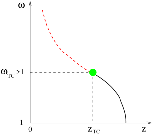
Figure 1: (Color online) Schematic phase diagram of the model of self-attracting self-avoiding walks (SASAW’s) on a lattice. The continuous polymerization transition is represented by a full line (black on line) and the discontinuous transition is located at the dashed line (red on line). Both transition lines are separated by a tricritical point, represented by the circle (green on line).

More recently, an alternative model has been proposed by Krawczyk et al kpor06 for the collapse transition of polymers. In this model, which we may call MMS (multiple monomers per site) model and is a generalization of the Domb-Joyce model dj72 , up to $K$ monomers may occupy the same site of the lattice. The canonical version of the model, with chains of fixed (large) number of monomers $M$, was studied for $K=3$ using computer simulations on the square and cubic lattices. Besides the case with no additional restrictions, which was named RA (immediate reversals allowed) model by the authors, a more restrictive model, where the chain is not allowed to return to the lattice site it occupied two steps ago, (RF model), was also studied. Collapse transitions were found only for the RF model on the cubic lattice, indicating that, at least for this lattice, the restrictions seem to be essential for the existence of these transition. The weight of a site with two and three monomers in the model is $\omega_{1}$ and $\omega_{2}$, respectively, and in the two-dimensional parameter space of the model defined by the variables $\beta_{1}=\ln\omega_{1}$ and $\beta_{2}=\ln\omega_{2}$, it seems that the collapsed polymerized phase (globule) is separated from the regular polymerized extended phase (coil) by lines of continuous and discontinuous transitions, both transition lines meeting at a tricritical point. We note that, in the SASAW’s model discussed above, the extended-collapsed transition in the canonical situation is continuous and of tricritical nature. One point which needs to be understood is the apparent absence of transitions in both models on the square lattice and in the RA model on the cubic lattice.

Motivated by the questions above, the grand-canonical version of the MMS model was studied on Bethe and Husimi lattices. Initially, both versions of the model (RA and RF) with $K=2$ were solved on a Bethe lattice with general coordination number $q$ pablo07 . Although these initial calculation for the models resulted in phase diagrams with some qualitative differences when compared to the usual behavior of SASAW’s, a revision using a different and better fundamented procedure to find the coexistence loci resulted in diagrams which are similar to the ones for SASAW’s, in both cases (RA and RF), with continuous transitions between the polymerized phases in the canonical formalism ss10 . The solution of the $K=2$ RF model on the Husimi lattice oss08 lead to a phase diagram similar to the one found for the same model on the Bethe lattice. A natural interpretation of this model is to consider that monomers on the same lattice attract each other, so that the statistical weights of sites with one and two monomers will be $\omega_{1}=z$ and $\omega_{2}=\omega z^{2}$, where $z$ is the fugacity of a monomer and $\omega=\exp(-\beta\epsilon)$ is the Boltzmann factor associated to the attractive interaction energy $\epsilon$ between monomers on the same site. While the tricritical point in the Bethe lattice solution of the model corresponds to $\omega_{TC}=1$, the solution on the Husimi lattice shows the tricritical point located at $\omega\approx 1.09$, in the region of attractive monomer-monomer interactions, as expected. More recently, the RF model for $K=3$ was solved on the Bethe lattice in the grand-canonical ensemble tiago09 . In the two-dimensional subspace of the three-dimensional parameter space used in the grand-canonical calculations, which corresponds to the canonical phase diagram, again the transitions between the polymerized phases are always continuous. Two transition lines, one composed by tricritical points and the other by critical endpoints, meet at a multicritical point, not far from the region in the parameter space where the tricritical point was found in the original simulations of the $K=3$ RF model on the cubic lattice.

Here we present calculations for the $K=3$ RA model on the Bethe lattice, partially motivated by the surprising result in the original simulations that no transition was found for this unrestricted model between the polymerized phases, while at least in the $K=2$ case the Bethe lattice calculations revealed no qualitative differences in the phase diagrams of the RA and RF models, both similar to the one found for the SASAW’s model. In section II we define the model in more detail and present its solution on the Bethe lattice in terms of recursion relations. The thermodynamic behavior of the model is determined by the fixed points of the recursion relations, together with a bulk free energy which is useful to locate the coexistence loci, and these results may be found in section III. Final discussions and the conclusion are presented in section IV.

II Definition of the model and solution in terms of recursion relations

We study the MMS-RA model proposed by Krawczyk et al in kpor06 in the core of a Cayley tree with arbitrary coordination number $q$. In this model, self- and mutually avoiding walks are considered but the excluded volume condition is relaxed, so that each site of the tree may be occupied by up to $K=3$ monomers, or, equivalently, each lattice site way be visited up to three times by the walks. No other restriction is imposed in the model, so that immediate reversals of the walk are allowed (RA model), differently from the more restrictive model studied in tiago09 where immediate reversals are forbidden (RF model), and thus a subset of the configurations of the walks considered here was included.

As usual, the endpoints of the walks are placed on the surface of the tree. Like in the original model kpor06 , a walk is described by the sequence of sites that it visits, so that the monomers placed on the same site are considered to be indistinguishable. A statistical weight $\omega_{i}$ is associated to a site occupied by $i$ monomers, with $i=1,2,3$. So, the grand-canonical partition function of the model will be given by:

$$Y=\sum_{N_{1},N_{2},N_{3}}\omega_{1}^{N_{1}}\omega_{2}^{N_{2}}\omega_{3}^{N_{3}}$$ (2)

where the sum is over the configurations of the walks on the tree, while $N_{i}$ , $i=1,2,3$, is the number of sites visited $i$ times by the walks. In Fig. 2, an example of a Cayley tree with three generations of sites is shown, as well as the contribution to the partition function which corresponds to the configuration of the walks in this case.

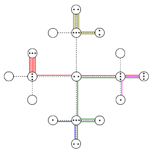
Figure 2: (Color online) A contribution to the partition function of the model on a Cayley tree with $q=4$ and 3 generations. The weight of this contribution will be $\omega_{1}^{3}\omega_{2}^{4}\omega_{3}^{6}$.

To solve the model on the Bethe lattice (the core of the Cayley tree) we start considering rooted subtrees, defining partial partition functions (ppf’s) for them, where we sum over all possible configurations of the chains for a fixed configuration of the root of the subtree (this is the reason for calling the partition functions partial). We thus define fourteen partial partition functions $g_{i}$, $i=0,1,\ldots,14$, shown in Fig. 3. The number of partial partition functions we need to define for the RA model is larger than the one we used for the RF model, where four root configurations were sufficient tiago09 , since more configurations are allowed in the present case.

When we define the possible root configurations, with up to four polymer bonds on the root edge. It is important to notice that, since immediate reversals of the walk are now allowed, it is possible to have closed loops on the tree and the ppf’s have to be carefully defined in order to avoid rings in the walks. This possibility does not exist in the RF model on the Bethe lattice. When rings are allowed, even the universality class of a polymer model changes to a model with $n=1$ components in the order parameter, that is, to the universality class of the Ising model. Therefore, in ppf’s with two or more bonds on the root edge, we need to distinguish between bond pairs that are connected (in earlier generations of the tree), or not. In Fig. 3, we have four ppf’s with two bonds in the root site ($g_{2}$ to $g_{5}$), for example. In bond pairs not connected by horizontal lines in our notation, such as in the root configurations for $g_{2}$ and $g_{6}$ (taken two by two) and one pair of $g_{10}$, the two walks will never meet on the tree at a site in earlier generations, or, in other words, if the walks are followed all the way to the surface of the tree, they end at different surface sites. When we draw horizontal lines connecting two bonds at the root edge, it means that they are connected to the same site in earlier generations and there are three possibilities for this: 1) The two bonds are connected to the same monomer of the root site (one line); 2) Both walks are connected to the same site in some earlier generation and visit the same sites of the tree (two lines); and 3) Same as case 2, but the walks visit different sites of the tree (three lines). In the last case, the two bonds are distinguishable, because the sequence of visited sites is different if we begin in one or other bond, although the visited sites are the same. These definitions are applied for every ppf with at least two bonds in the root site, and leads to the rather large number of ppf’s we need to define.

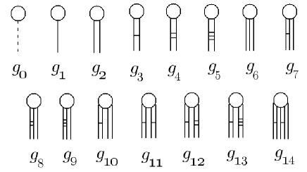
Figure 3: Illustration of the rooted subtrees which correspond to the partial partition functions. The meaning of the horizontal lines between bonds on the root edge is discussed in the text.

We then proceed obtaining recursion relations for the ppf’s, by considering the operation of attaching $q-1$ subtrees with a certain number of generations to a new root site and edge, thus building a subtree with an additional generation. Below the recursion relations are presented. In general, the partial partition function $g^{\prime}_{i}$ with an additional generation is the sum of contributions involving the parameters of the model and partial partition functions $g_{i}$. The primes denote the partial partition function of the subtree with one more generation. Whenever appropriate, the contributions to the sums begin with a product of two numerical factors, the first of which is the multiplicity of the configuration of the incoming bonds and the second is the multiplicity of the connections with the monomers located at the new root site. In the expressions below, $f_{i}\equiv\binom{\sigma}{i}g_{0}^{i}$, where $\sigma=q-1$ is the ramification of the tree. The recursion relations for the 14 ppf’s are:

$$g^{\prime}_{0} = f_{0}+\omega_{1}[f_{2}g_{1}^{2}+f_{1}g_{2}]+\omega_{2}[f_{4}\times 3g_{1}^{4}+3f_{3}\times 3g_{1}^{2}g_{2}+3f_{3}g_{1}^{2}(g_{3}+g_{4}+2g_{5})+2f_{2}\times 3g_{1}g_{6}+$$ (3)

$$2f_{2}g_{1}(g_{7}+g_{8}+2g_{9})+f_{2}\times 3g_{2}^{2}+2f_{2}g_{2}(g_{3}+g_{4}+2g_{5})+f_{1}g_{10}]+\omega_{3}[f_{6}\times 15g_{1}^{6}+$$

$$5f_{5}\times 15g_{1}^{4}g_{2}+6f_{4}\times 15g_{1}^{2}g_{2}^{2}+12f_{4}\times 6g_{1}^{2}g_{2}(g_{3}+g_{4}+2g_{5})+6f_{3}\times 15g_{1}g_{2}g_{6}+$$

$$6f_{3}\times 6g_{1}g_{2}(g_{7}+g_{8}+2g_{9})+5f_{5}\times 6g_{1}^{4}(g_{3}+g_{4}+2g_{5})+6f_{4}\times 2g_{1}^{2}(g_{3}+g_{4}+2g_{5})^{2}+$$

$$6f_{3}\times 6g_{1}(g_{3}+g_{4}+2g_{5})g_{6}+6f_{3}\times 2g_{1}(g_{3}+g_{4}+2g_{5})(g_{7}+g_{8}+2g_{9})+4f_{4}\times 15g_{1}^{3}g_{6}+$$

$$4f_{4}\times 6g_{1}^{3}(g_{7}+g_{8}+2g_{9})+3f_{3}\times 6g_{1}^{2}g_{10}+3f_{3}g_{1}^{2}(g_{11}+2g_{12}+4g_{13})+2f_{2}g_{1}g_{14}+f_{3}\times 15g_{2}^{3}+$$

$$3f_{3}\times 6g_{2}^{2}(g_{3}+g_{4}+2g_{5})+3f_{3}\times 2g_{2}(g_{3}+g_{4}+2g_{5})^{2}+2f_{2}\times 6g_{2}g_{10}+2f_{2}g_{2}(g_{11}+2g_{12}+4g_{13})+$$

$$2f_{2}\times 2(g_{3}+g_{4}+2g_{5})g_{10}+f_{2}\times 15g_{6}^{2}+2f_{2}\times 6g_{6}(g_{7}+g_{8}+2g_{9})+f_{2}\times 2(g_{7}+g_{8}+2g_{9})^{2}];$$

$$g^{\prime}_{1} = \omega_{1}f_{1}g_{1}+\omega_{2}[f_{3}\times 3g_{1}^{3}+2f_{2}\times 3g_{1}g_{2}+2f_{2}g_{1}(g_{3}+g_{4}+2g_{5})+f_{1}\times 3g_{6}+f_{1}(g_{7}+g_{8}+2g_{9})]+$$ (4)

$$\omega_{3}[f_{5}\times 15g_{1}^{5}+4f_{4}\times 15g_{1}^{3}g_{2}+3f_{3}\times 15g_{1}g_{2}^{2}+6f_{3}\times 6g_{1}g_{2}(g_{3}+g_{4}+2g_{5})+$$

$$4f_{4}\times 6g_{1}^{3}(g_{3}+g_{4}+2g_{5})+3f_{3}\times 2g_{1}(g_{3}+g_{4}+2g_{5})^{2}+3f_{3}\times 15g_{1}^{2}g_{6}+$$

$$3f_{3}\times 6g_{1}^{2}(g_{7}+g_{8}+2g_{9})+2f_{2}\times 6g_{1}g_{10}+2f_{2}g_{1}(g_{11}+2g_{12}+4g_{13})+2f_{2}\times 15g_{2}g_{6}+$$

$$2f_{2}\times 6g_{2}(g_{7}+g_{8}+2g_{9})+2f_{2}\times 6(g_{3}+g_{4}+2g_{5})g_{6}+2f_{2}\times 2(g_{3}+g_{4}+2g_{5})(g_{7}+g_{8}+2g_{9})+$$

$$f_{1}g_{14}];$$

$$g^{\prime}_{2} = \omega_{2}[f_{2}g_{1}^{2}+f_{1}g_{2}]+\omega_{3}[f_{4}\times 6g_{1}^{4}+3f_{3}\times 6g_{1}^{2}g_{2}+3f_{3}\times 2g_{1}^{2}(g_{3}+g_{4}+2g_{5})+2f_{2}\times 6g_{1}g_{6}+$$ (5)

$$2f_{2}\times 2g_{1}(g_{7}+g_{8}+2g_{9})+f_{2}\times 6g_{2}^{2}+2f_{2}\times 2g_{2}(g_{3}+g_{4}+2g_{5})+f_{1}\times 2g_{10}];$$

$$g^{\prime}_{3} = \omega_{1}+\omega_{2}[f_{2}g_{1}^{2}+f_{1}g_{2}]+\omega_{3}[f_{4}\times 3g_{1}^{4}+3f_{3}\times 3g_{1}^{2}g_{2}+3f_{3}g_{1}^{2}(g_{3}+g_{4}+2g_{5})+2f_{2}\times 3g_{1}g_{6}+$$ (6)

$$2f_{2}g_{1}(g_{7}+g_{8}+2g_{9})+f_{2}\times 3g_{2}^{2}+2f_{2}g_{2}(g_{3}+g_{4}+2g_{5})+f_{1}g_{10}];$$

$$g^{\prime}_{4} = \omega_{2}f_{1}(g_{3}+g_{4})+\omega_{3}[3f_{3}g_{1}^{2}(g_{3}+g_{4})+2f_{2}g_{1}(g_{7}+g_{8})+2f_{2}g_{2}(g_{3}+g_{4})+f_{1}g_{10}+f_{1}g_{11}];$$ (7)

$$g^{\prime}_{5} = \omega_{2}f_{1}g_{5}+\omega_{3}[3f_{3}g_{1}^{2}g_{5}+2f_{2}g_{1}g_{9}+2f_{2}g_{2}g_{5}+f_{2}(g_{3}+g_{4}+2g_{5})^{2}+f_{1}(g_{12}+2g_{13})];$$ (8)

$$g^{\prime}_{6} = \omega_{3}[f_{3}g_{1}^{3}+2f_{2}g_{1}g_{2}+f_{1}g_{6}];$$ (9)

$$g^{\prime}_{7} = \omega_{2}f_{1}g_{1}+\omega_{3}[f_{3}\times 3g_{1}^{3}+2f_{2}\times 3g_{1}g_{2}+2f_{2}g_{1}(g_{3}+g_{4}+2g_{5})+f_{1}\times 3g_{6}+f_{1}(g_{7}+g_{8}+2g_{9})];$$ (10)

$$g^{\prime}_{8} = \omega_{3}[2f_{2}g_{1}(g_{3}+g_{4})+f_{1}(g_{7}+g_{8})];$$ (11)

$$g^{\prime}_{9} = \omega_{3}[2f_{2}g_{1}g_{5}+f_{1}g_{9}];$$ (12)

$$g^{\prime}_{10} = \omega_{3}[f_{2}g_{1}^{2}+f_{1}g_{2}];$$ (13)

$$g^{\prime}_{11} = \omega_{2}+\omega_{3}[f_{2}g_{1}^{2}+f_{1}g_{2}];$$ (14)

$$g^{\prime}_{12} = \omega_{3}f_{1}(g_{3}+g_{4});$$ (15)

$$g^{\prime}_{13} = \omega_{3}f_{1}g_{5};$$ (16)

$$g^{\prime}_{14} = \omega_{3}f_{1}g_{1}.$$ (17)

The partial partition functions are expected to grow exponentially with the number of iterations, so we define ratios of them, which usually remain finite in the thermodynamic limit. Furthermore, we notice in the above equations that some ppf’s only appear in sums, they are $(g_{3}+g_{4}+2g_{5})$, $(g_{7}+g_{8}+2g_{9})$ and $(g_{11}+2g_{12}+4g_{13})$. Thus, it is convenient to define the following ratios:

$$R_{1}=\dfrac{g_{1}}{g_{0}},\quad R_{2}=\dfrac{g_{2}}{g_{0}},\quad R_{3}=\dfrac{(g_{3}+g_{4}+2g_{5})}{g_{0}},\quad R_{4}=\dfrac{g_{6}}{g_{0}}$$

$$R_{5}=\dfrac{(g_{7}+g_{8}+2g_{9})}{g_{0}},\quad R_{6}=\dfrac{g_{10}}{g_{0}},\quad R_{7}=\dfrac{(g_{11}+2g_{12}+4g_{13})}{g_{0}}\quad\text{and}\quad R_{8}=\dfrac{g_{14}}{g_{0}}.$$ (18)

From the recursion relations for the ppf’s, similar expressions may be obtained for the ratios. Denoting the binomial coefficients as $b_{i}\equiv\binom{\sigma}{i}$, the recursion relations for the ratios are:

$$R^{\prime}_{1} = \frac{1}{D}[\omega_{1}b_{1}R_{1}+\omega_{2}(3b_{3}R_{1}^{3}+6b_{2}R_{1}R_{2}+2b_{2}R_{1}R_{3}+3b_{1}R_{4}+b_{1}R_{5})+$$ (19)

$$\omega_{3}(15b_{5}R_{1}^{5}+60b_{4}R_{1}^{3}R_{2}+45b_{3}R_{1}R_{2}^{2}+36b_{3}R_{1}R_{2}R_{3}+24b_{4}R_{1}^{3}R_{3}+$$

$$6b_{3}R_{1}R_{3}^{2}+45b_{3}R_{1}^{2}R_{4}+18b_{3}R_{1}^{2}R_{5}+12b_{2}R_{1}R_{6}+2b_{2}R_{1}R_{7}+30b_{2}R_{2}R_{4}+$$

$$12b_{2}R_{2}R_{5}+12b_{2}R_{3}R_{4}+4b_{2}R_{3}R_{5}+b_{1}R_{8})];$$

$$R^{\prime}_{2} = \frac{1}{D}[\omega_{2}(b_{2}R_{1}^{2}+b_{1}R_{2})+\omega_{3}(6b_{4}R_{1}^{4}+18b_{3}R_{1}^{2}R_{2}+6b_{3}R_{1}^{2}R_{3}+12b_{2}R_{1}R_{4}+$$ (20)

$$4b_{2}R_{1}R_{5}+6b_{2}R_{2}^{2}+4b_{2}R_{2}R_{3}+2b_{1}R_{6})];$$

$$R^{\prime}_{3} = \frac{1}{D}[\omega_{1}+\omega_{2}(b_{2}R_{1}^{2}+b_{1}R_{2}+b_{1}R_{3})+\omega_{3}(3b_{4}R_{1}^{4}+9b_{3}R_{1}^{2}R_{2}+6b_{3}R_{1}^{2}R_{3}+$$ (21)

$$6b_{2}R_{1}R_{4}+4b_{2}R_{1}R_{5}+3b_{2}R_{2}^{2}+4b_{2}R_{2}R_{3}+2b_{2}R_{3}^{2}+2b_{1}R_{6}+b_{1}R_{7})];$$

$$R^{\prime}_{4} = \frac{\omega_{3}}{D}[b_{3}R_{1}^{3}+2b_{2}R_{1}R_{2}+b_{1}R_{4}];$$ (22)

$$R^{\prime}_{5} = \frac{1}{D}[\omega_{2}b_{1}R_{1}+\omega_{3}(3b_{3}R_{1}^{3}+6b_{2}R_{1}R_{2}+4b_{2}R_{1}R_{3}+3b_{1}R_{4}+2b_{1}R_{5})];$$ (23)

$$R^{\prime}_{6} = \frac{\omega_{3}}{D}[b_{2}R_{1}^{2}+b_{1}R_{2}];$$ (24)

$$R^{\prime}_{7} = \frac{1}{D}[\omega_{2}+\omega_{3}(b_{2}R_{1}^{2}+b_{1}R_{2}+2b_{1}R_{3})];$$ (25)

$$R^{\prime}_{8} = \frac{\omega_{3}}{D}b_{1}R_{1}.$$ (26)

The denominator $D$ is defined as:

$$D = 1+\omega_{1}(b_{2}R_{1}^{2}+b_{1}R_{2})+\omega_{2}(3b_{4}R_{1}^{4}+9b_{3}R_{1}^{2}R_{2}+3b_{3}R_{1}^{2}R_{3}+6b_{2}R_{1}R_{4}+2b_{2}R_{1}R_{5}+$$ (27)

$$3b_{2}R_{2}^{2}+2b_{2}R_{2}R_{3}+b_{1}R_{6})+\omega_{3}(15b_{6}R_{1}^{6}+75b_{5}R_{1}^{4}R_{2}+90b_{4}R_{1}^{2}R_{2}^{2}+72b_{4}R_{1}^{2}R_{2}R_{3}+$$

$$36b_{3}R_{1}R_{3}R_{4}+90b_{3}R_{1}R_{2}R_{4}+36b_{3}R_{1}R_{2}R_{5}+30b_{5}R_{1}^{4}R_{3}+12b_{4}R_{1}^{2}R_{3}^{2}+12b_{3}R_{1}R_{3}R_{5}+$$

$$60b_{4}R_{1}^{3}R_{4}+24b_{4}R_{1}^{3}R_{5}+18b_{3}R_{1}^{2}R_{6}+3b_{3}R_{1}^{2}R_{7}+2b_{2}R_{1}R_{8}+15b_{3}R_{2}^{3}+18b_{3}R_{2}^{2}R_{3}+$$

$$6b_{3}R_{2}R_{3}^{2}+12b_{2}R_{2}R_{6}+2b_{2}R_{2}R_{7}+4b_{2}R_{3}R_{6}+15b_{2}R_{4}^{2}+12b_{2}R_{4}R_{5}+2b_{2}R_{5}^{2}).$$

The grand-canonical partition function of the model on the Cayley tree may be obtained if we consider the operation of attaching $q$ subtrees to the central site of the lattice, similar to the one used for deriving the recursion relations for the ppf’s. The result will be:

$$Y=g_{0}^{q}(1+P+Q+S),$$ (28)

where:

$$P = \omega_{1}(c_{2}R_{1}^{2}+c_{1}R_{2});$$ (29a)

$$Q = \omega_{2}(3c_{4}R_{1}^{4}+9c_{3}R_{1}^{2}R_{2}+3c_{3}R_{1}^{2}R_{3}+6c_{2}R_{1}R_{4}+2c_{2}R_{1}R_{5}+$$ (29b)

$$3c_{2}R_{2}^{2}+2c_{2}R_{2}R_{3}+c_{1}R_{6});$$

$$S = \omega_{3}(15c_{6}R_{1}^{6}+75c_{5}R_{1}^{4}R_{2}+90c_{4}R_{1}^{2}R_{2}^{2}+72c_{4}R_{1}^{2}R_{2}R_{3}+36c_{3}R_{1}R_{3}R_{4}+$$ (29c)

$$90c_{3}R_{1}R_{2}R_{4}+36c_{3}R_{1}R_{2}R_{5}+30c_{5}R_{1}^{4}R_{3}+12c_{4}R_{1}^{2}R_{3}^{2}+12c_{3}R_{1}R_{3}R_{5}+$$

$$60c_{4}R_{1}^{3}R_{4}+24c_{4}R_{1}^{3}R_{5}+18c_{3}R_{1}^{2}R_{6}+3c_{3}R_{1}^{2}R_{7}+2c_{2}R_{1}R_{8}+15c_{3}R_{2}^{3}+$$

$$18c_{3}R_{2}^{2}R_{3}+6c_{3}R_{2}R_{3}^{2}+12c_{2}R_{2}R_{6}+2c_{2}R_{2}R_{7}+4c_{2}R_{3}R_{6}+15c_{2}R_{4}^{2}+$$

$$12c_{2}R_{4}R_{5}+2c_{2}R_{5}^{2}).$$

where $c_{i}\equiv\binom{q}{i}$. We notice that the contributions to $P$, $Q$, $S$ correspond to placing one, two and three monomers on the central site, respectively. Using the expressions above, we may obtain the densities at the central site of the tree, considering the configuration of this site for each contribution to the grand-canonical partition function 28. The density of sites occupied by one ($\rho_{1}$), two ($\rho_{2}$) and three ($\rho_{3}$) monomers are given, respectively, by:

$$\rho_{1} = \frac{P}{1\,+\,P\,+\,Q\,+\,S},$$ (30a)

$$\rho_{2} = \frac{Q}{1\,+\,P\,+\,Q\,+\,S},\mbox{and}$$ (30b)

$$\rho_{3} = \frac{S}{1\,+\,P\,+\,Q\,+\,S}.$$ (30c)

The Bethe lattice solution of the model is defined by its thermodynamic behavior in the core of the tree, represented by the densities just defined. The total density of monomers on the Bethe lattice, that is, the total number of monomers divided by the number of sites, is $\rho=\rho_{1}+2\rho_{2}+3\rho_{3}$, and will be in the range $0\leq\rho\leq 3$.

III Thermodynamic properties of the model

The thermodynamic phases of the system on the Bethe lattice will be given by the stable fixed points of the recursion relations, which are reached after infinite iterations of the recursion relations and thus correspond to the thermodynamic limit. We find three different stable solutions for the fixed point equations $R_{i}^{\prime}=R_{i}$, associated to one non-polymerized phase (NP) and two polymerized ones (P1 and P2).

The NP phase is characterized by the fixed point $R_{i}=0$ for all $i$, excluding $i=3$ and $i=7$. These last two may be obtained solving the equations:

$$2b_{2}\omega_{3}R_{3}^{2}+(b_{1}\omega_{2}+2b_{1}^{2}\omega_{3}^{2}-1)R_{3}+(\omega_{1}+b_{1}\omega_{2}\omega_{3})=0,$$ (31)

and

$$R_{7}=\omega_{2}+2b_{1}\omega_{3}R_{3}.$$ (32)

The quadratic equation for $R_{3}$ can be easily solved, but the explicit expression for $R^{NP}_{3}$ is too large to be shown here. Looking the equations 29 and 30 we see that $\rho=0$ in the NP phase, as expected.

In the two polymerized phases all ratios are non-vanishing and, in order to obtain the fixed point values, we have to iterate the recursion relations or solve the fixed point equations numerically. It is important to remark that the metastable phases with double e triple occupation of sites, that appear in the RF model tiago09 , are absent here. As is discussed in pablo07 , the immediate reversal of the walk makes the probabilities of find these configurations in the central site vanish.

The stability limits of all phases are obtained calculating the jacobian of the recursion relations:

$$J_{i,j}=\left(\frac{\partial R^{\prime}_{i}}{\partial R_{j}}\right).$$ (33)

A fixed point is stable if the dominant eigenvalue of the jacobian has a modulus smaller than unity, and the stability limit of the corresponding phase (spinodal) is located in the loci where this modulus becomes equal to unity.

In order to find the coexistence surfaces in the phase diagrams, we obtain the free energies of the thermodynamic phases of the model. This free energy may not be calculated directly from the partition function Eq. (28), since it refers to the whole Cayley tree and, remembering that in the thermodynamic limit the number of surface sites correspond to a finite fraction of the total number of sites, reflects the influence of the surface. The free energy per site in the core of the tree, which corresponds to the Bethe lattice solution, may be calculated following the Gujrati’s argument g95 , which was also derived in another way in tiago09 . The result for the grand-canonical free energy per site on the Bethe lattice (divided by $k_{B}T$) is:

$$\phi_{b}=-\frac{1}{2}\left[q\ln\left(D\right)-(q-2)\ln\left(1+P+Q+S\right)\right]$$ (34)

Using the spinodals to find the continuous transitions and the free energy to determine the coexistence surfaces we built the whole phase diagram of the system. Before presenting the complete three-dimensional phase diagram, in the space defined by the statistical weights $\omega_{1}$, $\omega_{2}$, and $\omega_{3}$, it is instructive look at the thermodynamic behavior in some cuts of the parameter space. All results presented below are for a lattice of coordination $q=4$ and qualitatively identical diagrams are obtained for other values of $q>2$.

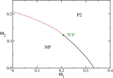
Figure 4: (Color online) Phase diagram for $\omega_{3}=0$. The red curve (above the tricritical point-TCP) is a first order transition and the black line (below the TCP) is a continuous transition between the NP and P2 phases. The TCP is indicated by the green square.

The diagram for $\omega_{3}=0$ ($K=2$) is shown in Fig. 4. For small values of $\omega_{2}$, we find a continuous transition, between the NP e P2 phases, which ends up at a tricritical point (TCP) located at $\omega_{1}^{TCP(K=2)}=0.2177$ and $\omega_{2}^{TCP(K=2)}=0.1146$ (for $q=4$). Above the tricritical point the transition becomes discontinuous. It is important to stress that this particular case ($\omega_{3}=0$) was studied by one of the authors in pablo07 , considering distinguishable monomers and using the natural initial conditions method to find the coexistence lines. There, only a discontinuous transition was found between the non-polymerized phase and a polymerized one (called P2 here). We notice that the diagram of pablo07 changes if Gujrati’s prescription is used to obtain the bulk free energy and the coexistence lines are determined using this free energy. Since this latter procedure has a better fundamentation than the earlier based on natural initial conditions tiago09 , the results provided by it are more reliable. We also notice that the phase diagram found here is very similar to one obtained for the RF model in tiago09 . However, the RF tricritical point was located at $\omega^{RF}_{1}=1/3$ and $\omega^{RF}_{2}=1/9$ tiago09 , which is far from the location found here. A generalization of the model for $K=2$, with the RA and RF models as particular cases, shows a line of tricritical points joining the two ones for both models ss10 .

For increasing values of $\omega_{3}$, the qualitative behavior of the phase diagrams, in the $(\omega_{1},\omega_{2})$ plane, is similar to the one depicted in Fig. 4. Thus, there is a tricritical point (TCP) line in the three dimensional phase diagram. This line ends up at a multicritical point (MCP), located at ($\omega_{1}^{MCP}=0.2700819$, $\omega_{2}^{MCP}=0.0182769$, $\omega_{3}^{MCP}=0.0450771$), so the TCP line lies in the region $0\leq\omega_{3}<\omega_{3}^{MCP}$. For $\omega_{3}>\omega_{3}^{MCP}$, more complex diagrams are found, as will be discussed below. The location of this multicritical point may be determined by noting that it corresponds to a higher order NP root of the fixed point equations. This will be discussed in some detail in the appendix.

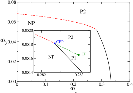
Figure 5: (Color online) Phase diagram for $\omega_{2}=0$. At the red (left of the critical endpoint-CEP) and the magenta (right of the CEP) curves we find first order transitions between the polymerized phase (P1) and the non-polymerized phase (NP) and between both polymerized phases, respectively. The black line (below the CEP) corresponds to continuous transitions between the NP and the polymerized phases. The blue (square) and magenta (circle) points are the critical endpoint (CEP) and a critical point (CP), respectively. All these features are better seen in the inset, which shows a small region close to the point where the discontinuous (NP-P2) and continuous (NP-polymerized) transitions lines meet.

A rich phase diagram was found in the $\omega_{2}=0$ plane, as show in Fig. 5. For small values of $\omega_{1}$ there is a first order transition between the NP em P2 phases, ending at a critical end-point (CEP), located at $\omega_{1}^{CEP}\approx 0.2823$ and $\omega_{3}^{CEP}\approx 0.0518$. In a tiny region of the phase diagram, where $\omega_{1}>\omega_{1}^{CEP}$ and $\omega_{3}\lessapprox\omega_{3}^{CEP}$, we found the second polymerized phase (P1). The two polymerized phases (P1 and P2) coexists in line which limits this region until a critical point is reached (at $\omega_{1}^{CP}\approx 0.2831$ and $\omega_{3}^{CP}\approx 0.0516$). This is shown in the inset of figure 5. Below the coexistence line (for $\omega_{1}>\omega_{1}^{CEP}$ and $\omega_{3}<\omega_{3}^{CEP}$), there is a continuous transition line between the NP and the polymerized phases.

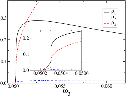
Figure 6: (Color online) Densities as a function of $\omega_{3}$, for $\omega_{1}=0.2799$ and $\omega_{2}=0.004$. In the inset we show a detail of the region with discontinuous transitions.

Comparing the phase diagram of Fig. 5 with the one of the RF model (for $\omega_{2}=0$) tiago09 , we can see that the qualitative picture is the same. However, in the RF model, the P1-P2 coexistence region is larger than the one for the RA model. Besides, as shown in tiago09 , for the RF model, the phase P1 is characterized by $\rho_{1}\gg\rho_{2},\rho_{3}$ at the coexistence with the P2 phase, where $\rho_{1}\sim\rho_{2}\sim\rho_{3}$. On the other hand, here we found that in the P1 phase all densities are of the same order as in P2, and thus the two phases have the same symmetries. In figure 6, we show the densities (defined in Eq. 30) for increasing values of $\omega_{3}$, with $\omega_{1}$ and $\omega_{2}$ fixed in the P1-P2 coexistence region. In face of this result, we can conclude that the restriction imposed in the RF model changes the nature of the P1 phase, which became approximately a SAW in that case, with dominance of sites with a single monomer, while when immediate reversals (RA model) for the walks are allowed, the P1 phase behaves like a regular polymerized phase in the MMS model. We advance that this difference of the P1 phase in the two models may explain the different regimes found in the phase boundaries in the canonical simulations of Krawczyk et al kpor06 . This point will be discussed in more detail below.

The ($\omega_{1},\omega_{3}$) phase diagrams are similar to the one in Fig. 5, for all $\omega_{2}$ smaller then the multicritical point value ($\omega_{2}<\omega_{2}^{MC}$). Therefore, we have lines of CP and CEP in the whole phase diagram and a P1-P2 coexistence surface between these lines. Thus, there exist a NP-P2 coexistence surface and a NP-polymerized critical surface in the three dimensional diagram. For increasing values of $\omega_{2}$, the CP line gets closer to the CEP line, making the numerical determination of their locations very hard. At the multicritical point these lines meet, together with the TCP line. When $\omega_{2}^{MCP}<\omega_{2}<\omega_{2}^{TCP(K=2)}$, the tricritical point line crosses the ($\omega_{1},\omega_{3}$) plane and the $\omega_{1}\times\omega_{3}$ diagrams resembles the one shown in Fig. 4.

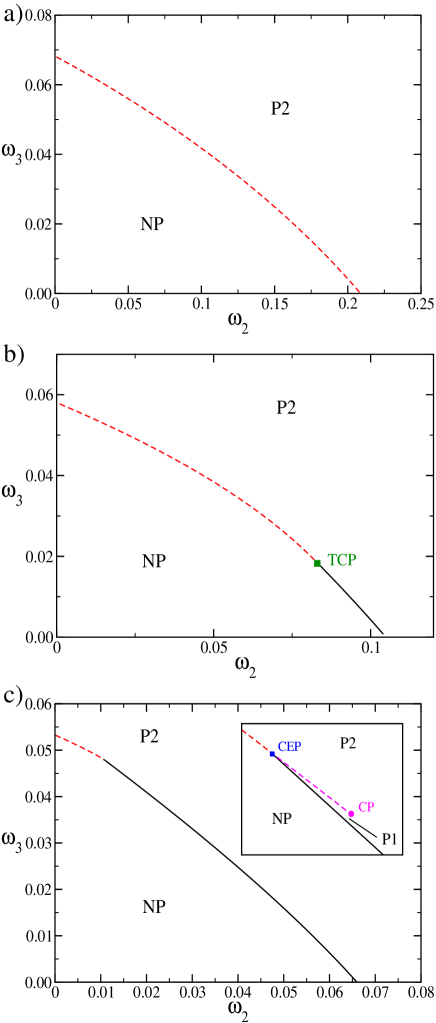
Figure 7: (Color online) Phase diagrams for: a) $\omega_{1}=0.0$, b) $\omega_{1}=0.23$ and c) $\omega_{1}=0.275$. The red and magenta (dashed) curves are NP-P2 and P1-P2 discontinuous transitions, respectively. The black line is the NP-polymerized continuous transition.

In Fig. 7, we show several diagrams, in the ($\omega_{2},\omega_{3}$) plane, for different fixed values of $\omega_{1}$. For $\omega_{1}=0$ (Fig. 7(a)), there is only a NP-P2 coexistence line and, for $\omega_{1}<\omega_{1}^{TCP(K=2)}$, similar diagrams are obtained, forming the NP-P2 coexistence surface. In the range $\omega_{1}^{TCP(K=2)}<\omega_{1}<\omega_{1}^{MCP}$, the NP-P2 transition may be continuous or discontinuous, and both transition lines meet at a tricritical point. In Fig. 7 (b) we show an example of these diagrams for $\omega_{1}=0.23$. Finally, for $\omega_{1}>\omega_{1}^{MCP}$, we find the same behavior of the ($\omega_{1}$, $\omega_{3}$) diagram for small $\omega_{2}$ (see Fig. 5), with two coexistence lines (NP-P2 and P1-P2) which meet at a critical end-point, where the line of continuous transition between the NP and the polymerized phases ends (see Fig. 7 (c)).

Again, the diagrams found here with fixed $\omega_{1}$ are similar to those of the RF model tiago09 . The main difference is that the tricritical and critical end-point lines of the RA model are functions of the three parameters ($\omega_{1}$, $\omega_{2}$ and $\omega_{3}$), while in the RF model these lines lie in the plane $\omega_{1}=1/3$. In the same way, in the RA model the NP-polymerized continuous transition appear as a curved surface, while in the RF model, it is located in the plane $\omega_{1}=1/3$.

A sketch of the whole three-dimensional phase diagram is shown in Fig. 8, summarizing the features we have discussed above. Like discussed above, the CEP and CP lines are very close in the phase diagram and we can not see the two lines in the figure 8. Therefore, we show only the CEP line in the diagram, but it is important to keep in mind that there is also a CP line in the neighborhood of this line. In particular, due to the existence of this additional coexistence surface between both polymerized phases, the NP-P critical surface and the NP-P coexistence surface do not meet tangentially at the CEP line, and the angle between the normal vectors to both surfaces at this line becomes larger as further we are from the multicritical point, where the tricritical, critical endpoint and P1-P2 critical line meet tangentially. Therefore, this angle is largest when $\omega_{2}=0$, as may be seen in Fig. 5.

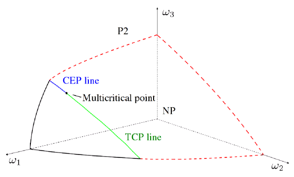
Figure 8: (Color online) Sketch of the three-dimensional phase diagram. The NP-P2 discontinuous transition surface (red, dashed lines) and the NP-polymerized critical surface (black, continuous line) are shown. The P1-P2 coexistence surface and critical line close to the CEP line are to small to be represented here.

IV Final discussions and conclusions

Although the Bethe lattice solution of the RA model is close to the one of the restrictive RF model, the polymerized phases P1 are very different in the two models. Moreover, in the RF model the continuous transition surface exists between the NP and P1 phases only, while here the main part of this surface are between the NP and a polymerized phase that can not be identified as P1 or P2, because they are above the critical point line. These results may explain the difference found in the canonical simulations of Krawczyk et al kpor06 between the RA and RF models. For the RF model, Krawczyk et al kpor06 suggest a canonical phase diagram with discontinuous and continuous transition lines which meet at a tricritical point, between a SAW-like phase (sites occupied mainly by a single monomer) and a collapsed one (sites predominantly with two or three monomers). The location of the TCP is not defined precisely by the simulations, but the authors suggest that it is in the region of attractive interaction between monomers, namely, the first quadrant in the $(\beta_{1},\beta_{2})$ parameter space. The Bethe lattice solution of this model tiago09 shows that, in fact, there is a SAW-like phase (the critical surface NP-P1) and a collapsed phase (the coexistence surface NP-P2). However, the discontinuous and continuous transitions lines, suggested in the simulations, are a tricritical and a CEP line in this approximation, respectively. On the other hand, no SAW-collapsed transition was found in the simulations of the RA model in kpor06 . This is in agreement with our results, because here the critical surface NP-polymerized does not lead to a SAW-like phase in the canonical diagram. In contrast with the RF model, where the sites are predominantly visited by one monomer, here the densities in phase P1 depends only on the statistical weights ($\omega_{i}$), like in phase P2. Thus, both the critical surface NP-polymerized and the coexistence surface NP-P2, are associated with collapsed phases, since the sites are occupied predominantly by more than one monomer in both cases. The former leads to a collapsed phase with low density (CLD) of monomers and the last has a larger density (CHD). We believe that the similarity between these phases makes it difficult to distinguish them in the simulations, which could have lead to the conclusion of no transition for the canonical RA model in kpor06 .

In order to compare our grand-canonical results for the RA with the canonical ones obtained in the simulations for the RF model kpor06 , we map our grand-canonical diagram into canonical one. As was discussed in tiago09 , the canonical variables used in the simulations kpor06 are related to the Boltzmann weights of our solution as:

$$\beta_{1}=\ln{\left[\frac{\omega_{2}}{\omega_{1}^{2}}\right]}\quad\quad\text{and}\quad\quad\beta_{2}=\ln{\left[\frac{\omega_{3}}{\omega_{1}^{3}}\right]},$$ (35)

and in the canonical formalism we are always restricted to the boundary of the NP phase. The canonical phase diagram which we found in the $\beta_{1},\beta_{2}$ parameter space is shown in Fig. 9. Like discussed above, we found two collapsed phases with high (CHD) and low (CLD) monomer densities that are related to the grand-canonical NP-P2 coexistence surface and NP-polymerized critical surface, respectively.

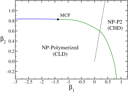
Figure 9: (Color online) Canonical phase diagram. The green curve (below the MCP, represented by the black circle) is the tricritical line and the blue (above the MCP) is the CEP line. On the line $\beta_{2}=3\beta_{1}$ (dashed) the MMS-RA model is related to the SASAW’s model.

The CLD-CHD transitions are always continuous, but of different types: for values of $\beta_{2}$ below the multicritical point there is a tricritical line and above this point a critical end-point line separates the two phases. The multicritical point is located at $\beta_{1}=-1.3840554$ and $\beta_{2}=0.8277081$. The same behavior was found in the Bethe lattice solution of the RF model tiago09 , but there the whole TCP line lies in the region of negative values for $\beta_{2}$ negative axis ($\beta_{1}=0$, $\beta_{2}<0$) and the MCP is placed at the origin ($\beta_{1}=\beta_{2}=0$). Curiously, here the MCP is located in a region with repulsive interaction between monomers at same site, when only two monomers are present. Thus, in this region, sites occupied by two monomers are penalized, while sites with one or three monomers are favored. In fact, in the Fig. 6, that show the densities in a region close to the MCP, we can see that $\rho_{1},\rho_{3}\gg\rho_{2}$.

A connection can be established between the MMS and the SASAW’s models, as was already discussed in tiago09 . If we suppose that only monomers located at the same site have through an attractive pairwise interaction of energy $-\epsilon$, in the grand-canonical ensemble we should have $\omega_{1}=z$, $\omega_{2}=z^{2}\omega$, and $\omega_{3}=3z^{3}\omega$, where, as before, $\omega=\exp(\beta\epsilon)$. In the canonical situation, from Eqs. (35), this leads to $\beta_{2}=3\beta_{1}=3\omega$. This line is shown in Fig. 9, and it crosses the tricritical line, so that the collapse transition in the subspace of the parameter space where the MMS-RA model on the Bethe lattice with $K=3$ is related to the SASAW’s model is tricritical, as it is also in the SASAW’s model.

In conclusion, to study the thermodynamic behavior of models for complex fluids such as the one considered here, for which exact solutions are usually difficult to obtain, we think it is useful to combine numerical simulations with approximate analytic solutions. In particular, the findings in this work suggest that the qualitative behavior of the MMS model without restrictions (RA) may be similar to tho one of the restricted model (RF). Also, on the Bethe lattice, the MMS model shows a behavior which is close to the one of the standard SAW’s model for the collapse transition of polymers. Of course one has to be aware that Bethe lattice solutions, as all mean-field like approximations, overestimate the interactions, and therefore may predict phase transitions in situations where better approximations or exact solutions find none, but in our opinion the results found on the Bethe lattice for the MMS model suggest that additional investigations using simulations or other more precise techniques are desirable.

Appendix A Determination of the location of the multicritical point

The multicritical point may be defined as the common point of the lines of tricritical points and critical endpoints, as may be seen in the full phase diagram depicted in Fig. 8. This definition, however, does not lead directly to a precise algorithm to determine the location of the multicritical point, due to the rather intricate nonlinear fixed point equations which need to be handled for this purpose. Sometimes, in Bethe or Husimi lattice solutions, it may be possible to reduce the fixed point equations to a polynomial, and then the higher order transition loci can be identified with the higher order roots of the NP fixed point, and example of this procedure is described for the particular case $K=2$ of the RF-RA model in ss10 . We were not able to pursue accomplish this calculation in the present case.

Another possibility, which was used for the $K=3$ RF model in tiago09 , is to assume that, close to the NP fixed point, the remaining ratios may be expanded in powers of one of them. By expanding the fixed point equations in powers of the chosen ratio, one then requires the higher order transition loci to be a higher order root of the resulting set of equations in the parameters of the model and the expansion coefficients. In the present case, we expanded the remaining ratios in powers of $R_{1}$ and found a consistent solution of this kind by requiring the multicritical point to satisfy the expanded fixed point equations up to order $R_{1}^{5}$. This rather high order is necessary due to parity effects we found in the expansions of the ratios. We assumed that, up to order $R_{1}^{5}$, the ratios may be expanded as follows:

$$R_{2} = a_{22}R_{1}^{2}+a_{24}R_{1}^{4},$$ (36a)

$$R_{3} = a_{30}+a_{32}R_{1}^{2}+a_{34}R_{1}^{4},$$ (36b)

$$R_{4} = a_{43}R_{1}^{3}+a_{45}R_{1}^{5},$$ (36c)

$$R_{5} = a_{51}R_{1}+a_{53}R_{1}^{3}+a_{55}R_{1}^{5},$$ (36d)

$$R_{6} = a_{62}R_{1}^{2}+a_{64}R_{1}^{4},$$ (36e)

$$R_{7} = a_{70}+a_{72}R_{1}^{2}+a_{74}R_{1}^{4},$$ (36f)

$$R_{8} = a_{81}R_{1}+a_{83}R_{1}^{3}+a_{85}R_{1}^{5}.$$ (36g)

Now these expressions are substituted into the 8 fixed point equations which are obtained by imposing $R_{i}^{\prime}=R_{i}$ in the recursion relations for the ratios Eqs. (19-26). Expanding these fixed point equations up to order $R_{1}^{5}$, using a algebra software for this task, we obtain several expansion coefficients of the fixed point equations. Considering the parity of the expansions shown in Eqs. (36) and denoting by $C_{ij}$ the coefficient of order $R_{1}^{j}$ in the fixed point equation obtained from the recursion relation for $R_{i}$, we are lead to 21 equations $C_{i,j}=0$, corresponding the the coefficients $(1,1)$, $(1,3)$, $(1,5)$, $(2,2)$, $(2,4)$, $(3,0)$, $(3,2)$, $(3,4)$, $(4,3)$, $(4,5)$, $(5,1)$, $(5,3)$, $(5,5)$, $(6,1)$, $(6,3)$, $(6,5)$, $(7,0)$, $(7,2)$, $(7,4)$, $(8,1)$, $(8,3)$ and $(8,5)$. In particular, $C_{3,0}=0$ and $C_{7,0}=0$ lead to the pair of equations (31,32) for the fixed point values of the NP phase presented above. The complete set of equations is too long to be given here. Solving this set of nonlinear algebraic equations for the 18 expansion coefficients $a_{ij}$ and the 3 statistical weights $\omega_{i}$, we obtain the result: $a_{22}=0.4882335108$, $a_{24}=0.2869523407$, $a_{30}=0.3329767741$, $a_{32}=-0.03809592295$, $a_{34}=0.1519415331$, $a_{43}=0.2048247034$, $a_{45}=-0.2633449211$, $a_{51}=0.3220483966$, $a_{53}=0.1813751089$, $a_{55}=-0.6519478195$, $a_{62}=0.2012557404$, $a_{64}=-0.2612169532$, $a_{70}=0.1083347046$, $a_{72}=0.03872548434$, $a_{74}=-0.1169008783$, $a_{81}=0.1352312919$, $a_{83}=-0.2015959772$, and $a_{85}=0.1269313668$ for the expansion coefficients and $\omega_{1}=0.2700819945$, $\omega_{2}=0.01827694593$, and $\omega_{3}=0.04507709731$ for the statistical weights. We did some numerical calculations for the fixed point values of the ratios in the neighborhood of the multicritical point, and found that they are consistent with the expansion coefficients we found.

References

- (1) P. J. Flory, Principles of Polymer Chemistry, edition, Cornell University Press, NY (1966).
- (2) P. G. de Gennes, Scaling Concepts in Polymer Physics, Cornell University Press, NY (1979).
- (3) E. W. Montroll and B. J. West in Studies in Statistical Mechanics - volume VII - Fluctuation Phenomena, edited by E. W. Montroll and J. L. Lebowitz, North Holland (1979).
- (4) B. Nienhuis, Phys. Rev. Lett. (1982).
- (5) C. Domb, J. Phys. C: Solid St. Phys 3, 256 (1970).
- (6) T. J. Oliveira, J. F. Stilck, and P. Serra Phys. Rev. E 80, 041804 (2009).
- (7) P. G. de Gennes, Phys. Lett. A 38,339 (1972). See also the detailed description of this correspondence in J. C. Wheeler and P. Pfeuty, Phys. Rev. A 24, 1050 (1981).
- (8) P. G. de Gennes, J. Physique Lettres 36, 1049 (1975).
- (9) B. Derrida and H. Saleur, J. Phys. A 18, L1075 (1985); H. Saleur, J. Stat. Phys. 45, 419 (1986).
- (10) B. Duplantier and H. Saleur, Phys. Rev. Lett 59, 539 (1987); B. Duplantier, Phys. Rev. A 38, 3647 (1988).
- (11) J. Krawczyk, T. Prellberg, A. L. Owczarek, and A. Rechnitzer, Phys Rev. Lett. 96, 240603 (2006).
- (12) C. Domb and G. S. Joyce, J. Phys. C 5, 956 (1972).
- (13) P. Serra and J. F. Stilck, Phys. Rev. E 75, 011130 (2007).
- (14) P. Serra and J. F. Stilck, in preparation (2010).
- (15) T. J. Oliveira, J. F. Stilck, and P. Serra Phys. Rev. E 77, 041103 (2008).
- (16) P. D. Gujrati, Phys. Rev. Lett. 74, 809 (1995).