Origin of the Pseudogap and Its Influence on Superconducting State

Abstract

When holes move in the background of strong antiferromagnetic correlation, two effects with different spatial scale emerge, leading to a much reduced hopping integral with an additional phase factor. An effective Hamiltonian is then proposed to investigate the underdoped cuprates. We argue that the pseudogap is the consequence of dressed hole moving in the antiferromagnetic background and has nothing to do with the superconductivity. The momentum distributions of the gap are qualitatively consistent with the recent ARPES measurements both in the pseudogap and superconducting state. Two thermal qualities are further calculated to justify our model. A two-gap scenario is concluded to describe the relation between the two gaps.

1. Introduction

One of the most fascinating properties of the cuprates is the opening of the pseudogap above the superconducting (SC) critical temperature $T_{c}$ in the underdoped and optimally doped regime, where most abnormalities observedTTimusk . The origin of the pseudogap and its relation to the SC gap are fundamental questions to realize the physics underline the high-temperature superconductors. Although much progress has been made, the issues remain open. There are two distinct scenarios on the relation between the pseudogap and SC gapSTS . 1) The one-gap scenario: The pseudogap is viewed as the precursor of SC gap, reflecting pair fluctuation above $T_{c}$, and would acquire phase coherence below $T_{c}$.Emery ; PALee The argument was based on angle-resolved photoemission spectroscopy (ARPES)HDing ; Loeser ; Valla , electron tunneling Renner ; Campuzano , and thermal transport measurementsHawthorn , etc.; 2) The two-gap scenario: The pseudogap is not directly related to the SC gap, but emerges from some ordered states such as antiferromagnetismAF , staggered fluxSF , stripeSTRIPE-Emery ; STRIPE-Kivelson , spin or charge density waveSCDW-Moon ; SCDW-Greco , orbital circulating currentsOCC , and resonating valence bond spin liquidYRZ , etc., and competes with SC gap. Many experiments, including ARPESKaminski ; Hashimoto ; RHHe , electronic Raman scatteringLeTacon , and elastic neutron diffractionLipscombe ; Fauque , etc., seem to favor the two-gap scenario. More recently, the improved ARPES dataTanaka ; WSLee ; TKondo ; KTerashima ; Kanigel ; Kanigel2 showed that the gap opens near the gap (antinodal) region, and vanishes near the arc (nodal) region in the pseudogap state, which leads to the arc structure of the Fermi surface. In the SC state, the pseudogap dominates the gapped region, while in the arc region, the simple d-wave type gap dominates.

In normal state of conductors, the low energy excitation can be described in terms of quasiparticle picture by introducing the self-consistent single particle scattering potential. Such simple quasiparticle picture failed to describe the conventional superconducting state due to the emergent particle non-conservation induced by the superconducting condensation. However, the quasiparticle picture can be recovered by further introducing the self-consistent pair potential. It is natural to ask whether the quasiparticle picture remains available in cuprates, especially in the most interested pseudogap state. The widely used slave-bosonBrinckmann and Gutzwiller projection approximationZFC are suitable rather for the overdoped than the underdoped case as compared with experiments. Models account for those above mentioned ordered states capture some aspects of the pseudogap state, but a theoretical framework, which gives a full picture from the pseudogap to SC state, is not yet established. Recently, Yang et al. proposed a phenomenological modelYRZ to account for the underdoped cuprates. However, both the pseudogap and SC gap adopted there are experimentally fitted for different doping in reality. We believe that a reasonable quasiparticle picture can be also proposed in the pseudogap region if the main strong correlation effects have been taken into account. This is significantly important even if it is approximate to some degrees. The questions are now how to extract the main effects and to what degree the quasiparticle picture consists with the experimental measurements.

In this paper, we try to establish an effective single particle Hamiltonian to understand the underdoped cuprates. The strong correlations in the underdoped cuprates are taken into account. The limitation of no double occupancy leads to much reduced effective hopping integral, reflecting the effect with large spatial scale, and the antiferromagnetic (AFM) background introduces an additional phase factor in the hopping term, reflecting the effect with small spatial scale. By considering these two effects with different spatial scale, the doping and momentum dependence of the pseudogap, arc structure Fermi surface, and the evolution of the quasiparticle dispersion are obtained and they are qualitatively consistent with the experimental discovery. We argue the pseudogap, originated from the short-range AFM correlations, is the property of the single particle and irrelevant to the superconductivity. The model Hamiltonian is extended into the superconducting state by adopting a phenomenological SC term. The results are also qualitatively consistent with recent ARPES measurements. The calculations on the specific heat and superfluid density confirm the validity of proposed effective Hamiltonian. Since the most previous studies on the pseudogap and SC gap focus in the momentum space both experimentally and theoretically, we also restrict our investigations in the momentum space to compare with previous experimental and theoretical results. The possible spatial inhomogeneity below $T^{\star}$, which had been discovered experimentallySonier ; Parker , will not be taken into account.

The paper is organized as follows. In Sec. 2, two main strong correlation effects in underdoped cuprates are considered. The effective single-particle Hamiltonian is consequently proposed. This Hamiltonian is discussed in the pseudogap state, and SC state in Sec. 3, and Sec. 4, respectively. In Sec. 5, We calculate the specific heat and superfluid density to further justify our effective Hamiltonian. The conclusion is given in Sec. 6, together with some discussions.

2. Two Spatial Scale Effects and effective single particle Hamiltonian

The strong correlations play the key roles in the underdoped cuprates. Essentially, this includes two main aspects. One is the AFM background, and the other is limitation of the double occupancy. A sophisticated theory should take into account both of them. We start from the extended $t-J$ model, which is thought to capture the main aspects of the cuprates

$$H=-\left(t\sum_{\left\langle ij\right\rangle_{1}\sigma}+t^{\prime}\sum_{\left\langle ij\right\rangle_{2}\sigma}+t^{\prime\prime}\sum_{\left\langle ij\right\rangle_{3}\sigma}\right)c_{i\sigma}^{+}c_{j\sigma}+J\sum_{\left\langle ij\right\rangle_{1}}\vec{S}_{i}\cdot\vec{S}_{j},$$ (1)

where $\left\langle ij\right\rangle_{n}$ with $n=1$, $2$, and $3$ denoting the nearest neighbor (NN), second-NN, and third-NN, respectively.

The long-range AFM order disappears under slightly hole doping. However, the neutron scatteringLipscombe ; Fauque and quantum oscillations measurementsSebastian show that the AFM correlation and its associated staggered flux state remains finite on the $CuO_{2}$ plane in the underdoped regime. Their existence has also been found numericallyLeung1 ; Ivanov ; Leung2 . This gives the substantial contributions to the underdoped cuprates. Unfortunately, Such effect is usually neglected in the previous treatments. In the Table 1, the NN spin-spin correlation $\langle S_{i}\cdot S_{j}\rangle$ is shown by applying the exact diagonalization (ED) technique on the $20$-site lattice. In the underdoped cases, it is always negative, implying the AFM correlation. In the background of the antiferromagnetism, for each site, its four nearest neighbors compose a plaquette. When a hole is introduced into the center of this plaquette, it will sense an effective magnetic field $B_{eff}$ originated from its four neighboring opposite spins as shown in the Fig. 1(a). $B_{eff}$ can be phenomenologically estimated by the NN spin-spin correlation between a spin $1/2$ sitting on the site of the given hole and its surrounding spins

$$B_{eff}=J\sum_{j\in NN}\langle S_{i}\cdot S_{j}\rangle/g\mu_{B}\langle S_{z}\rangle$$ (2)

with $\langle S_{z}\rangle=1/2$, and $g$, $\mu_{B}$ representing Landè factor, Bohr magneton, respectively. This effective magnetic field alters its sign when the given site moves to the nearest neighbor. Correspondingly, there is a doping dependent gauge flux $\Phi=B_{eff}a^{2}$ threading through the plaquette ($a=0.40nm$ denoting the lattice constant) as shown in Fig. 1(b). In its journey of wandering, the hole is affected by the staggered flux field in which $\Phi$ and $-\Phi$ appear alternatively. This staggered flux phase can be also established by consideration of the current-current correlation as manifested in the variational Monte CarloIvanov and ED calculationsLeung2 . Therefore, in the small spatial scale, when the hole hops, it will be exerted by a phase shift $\delta/4$ (or $-\delta/4$ ) due to Aharonov-Bohm effect, where $\delta=2\pi\Phi/\Phi_{0}$ ($\Phi_{0}=hc/e$ is the flux quanta)Harris . This also implies that the original translational symmetry is broken, consisting with the recent STM experimentsSTM .

Table 1: The ED results of the spin-spin correlation function and hopping matrix in the 20-site cluster with different hole concentration. $t=1$, $t^{\prime}=-0.3$, $t^{\prime\prime}=0.2$, and $J=0.4$.

$n_{h}$	$\langle S_{i}\cdot S_{j}\rangle$	$I_{1}$	$I_{2}$	$I_{3}$
$0$	$-0.3454$	$0$	$0$	$0$
$1$	$-0.2745$	$0.0703$	$-0.0297$	$0.0125$
$2$	$-0.2179$	$0.1483$	$-0.0350$	$0.0355$
$3$	$-0.1670$	$0.2116$	$-0.0469$	$0.0510$
$4$	$-0.1399$	$0.2635$	$-0.0594$	$0.0732$
$5$	$-0.0855$	$0.3126$	$-0.0709$	$0.0960$

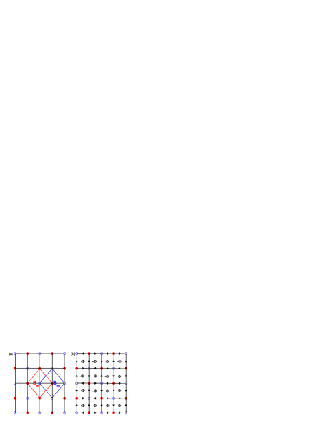
Figure 1: (Color online) (a) Schematic effective magnetic field as described in the text, and (b) staggered flux phase. The solid and blank circles are for the atoms of cuprate. It is divided into two sublattice due to the broken of translational symmetry.

On the other hand, it is well known that the effective hopping is much reduced in the cuprates due to the limitation of no double occupancy. To account for this effect, we directly calculate the hopping matrix, $I_{n}=\left\langle C_{i}^{+}C_{j}+C_{j}^{+}C_{i}\right\rangle$ ($n=1$, $2$, $3$ for the NN, second-NN, and third-NN, respectively), by ED technique as shown in Table. 1. The hermiticity is guaranteed under such selection. Since its value is $1-x^{2}$ if the strong correlations are not taken into accountZFC . For low doping, we neglect the high order term $x^{2}$. Therefore, $I_{n}$ obtained here is just the effective hopping when $t$ is taken as unit. The average process takes account for the all possible configurations. In this sense, it is the effect with large spatial scale. In fact, $I_{n}$ obtained here is similar to the previous renormalized factor adopted in the Slave-boson and Gutzwiller projection approximationsBrinckmann ; ZFC . We find that this value is underestimated in the slave-boson treatments, and overestimated in the Gutzwiller projection treatments for the NN hopping. For the second-NN hopping, it approaches to the value under the slave-boson treatment. Here, we would like to point out that the NN hopping matrix enhances with decreasing $J$. When $J=0$, its value is almost the same as that under the Gutzwiller approximation, especially for $t^{\prime}=0$, and $t^{\prime\prime}=0$. Present treatment is a full consideration of the strong correlation, both the no-double occupancy restriction and the antiferromagnetic correlation are taken into account, compared with only the former is considered in the Gutzwiller projection approximation. For more hole cases, the hopping matrix should be further divided by a factor approximately equal to hole number.

The original lattice is now divided into two sublattices $D$ and $E$ with the corresponding fermionic operators $d$ and $e$ due to the broken translational symmetry as mentioned aboveYQS . The effective hopping is much reduced due to the effect with large spatial scale. Furthermore, an additional phase shift is introduced when the hole hops to the nearest neighbor site due to the effect with the small spatial scale. Consequently, we may write the following effective single particle Hamiltonian as,

$$H=\sum_{k\sigma}\left(\gamma_{k}d_{k\sigma}^{+}e_{k\sigma}+hc\right)+\sum_{k\sigma}\epsilon_{k}\left(d_{k\sigma}^{+}d_{k\sigma}+e_{k\sigma}^{+}e_{k\sigma}\right),$$ (3)

where $\gamma_{k}=-2(I_{1}+J^{\prime}\kappa_{0})(e^{i\delta/4}\cos k_{x}+e^{-i\delta/4}\cos k_{y})$, and $\epsilon_{k}=-4I_{2}\cos k_{x}\cos k_{y}-2I_{3}\left(\cos 2k_{x}+\cos 2k_{y}\right)-\mu$, with $\mu$, a chemical potential determined by the hole density. $\kappa_{0}=\sum_{\sigma}\left\langle c_{i\sigma}^{+}c_{j\sigma}\right\rangle/x$ is the uniform bond order with $J^{\prime}=3J/8$ as usualYRZ . The summation is restricted in the magnetic Brillouin zone (MBZ). Numerically, $t$ (about $0.4eV$ in the real material) is taken as energy unit, $t^{\prime}=-0.3$, $t^{\prime\prime}=0.2$, and $J=0.4$ is adopted. As shown in the Table 1, the hopping matrix $I_{3}$ is strong than $I_{2}$ for more hole doping due to the size effect, $I_{3}$ is then modified to be $2I_{2}/3$.

So far, an effective model Hamiltonian is established based on our knowledge of the moving hole in the background of antiferromagnetism. We emphasize that no special parameters have been introduced in the discussion of normal state. The concept of staggered flux in cuprates is not a new concept. However, it is rather phenomenological and qualitative previously. Here, we explicitly demonstrate the origin of staggered flux and give the way to determine it quantitatively.

3. Results in the Pseudogap State

In the following discussion, we would explore the adaptation of the established effective single particle Hamiltonian (3) to describe the energy spectrum in strongly correlated systems. The effective Hamiltonian is diagonalized with the quasiparticle (QP) dispersion $\epsilon_{k}^{\eta}=\epsilon_{k}+\eta|\gamma_{k}|$ ($\eta=\pm$, $+$ for upper band, and $-$ for lower band). Correspondingly, the diagonal and off diagonal Green’s function is given as $G_{k,\omega}=\sum_{\eta}W^{\eta}/(\omega-\epsilon_{k}^{\eta})$, and $\tilde{G}_{k,\omega}=\sum_{\eta}\tilde{W}^{\eta}/(\omega-\epsilon_{k}^{\eta})$ respectively. The weight factor $W^{\eta}=\frac{1}{2}(1+\eta cos\varphi_{k})$, and $\tilde{W}^{\eta}=-\eta\frac{i}{2}sin\varphi_{k}$ with $e^{i\varphi_{k}}=\gamma_{k}/|\gamma_{k}|$. The QP dispersion together with its weight is shown in upper panel of Fig. 2. The upper and lower band coincide at $(\pi/2,\pi/2)$. This means that no full gap opens, unlike the Mott insulator state. The lower band is rather rigid against doping along the nodal line with much reduced bandwidth $0.65-0.75t(\sim 260-300meV)$. In the antinodal regime, clear flatness below Fermi energy $E_{f}$ (fixed at $0$) up to $x=0.25$ can be found. Therefore, a pseudogap (denoted by $\Delta^{PG}$) opens around this regime. The distance between the flatness part and $E_{f}$ decreases with increasing doping. These features qualitatively coincide with the ARPES dataMarshall . We also plot the evolution of the Fermi surface (FS) in the lower panel of Fig. 2. The intensity is strong near the nodal region, and vanishes in the antinode region due to the opening of the pseudogap, producing a hole pocket structure. On the other hand, the weight factor $W^{+}$ is much reduced beyond the MBZ, especially, near the nodal direction. Therefore, the hole pocket looks more like an arcNorman . It extends to a large hole FS above $x=0.25$, where the pseudogap vanishes gradually. Hence, the arc structure FS is a direct consequence of the opening of pseudogap. The evolution of the arc structure and its length also qualitatively agree with the recent ARPES experimentKMShen but with a slightly expanded doping range because of the overestimating of the spin-spin correlation due to the size effect.

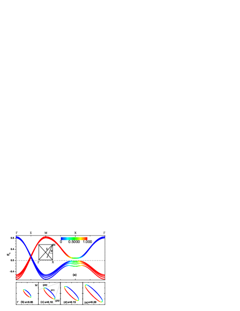
Figure 2: (Color online) Upper panel: the QP dispersion $\epsilon_{k}^{\pm}$ for different hole concentration (from bottom to top at $X$ point in the lower band are $x=0.05$, $0.10$, $0.15$, and $0.20$.), together with its weight factor. Thick, and thin lines are for lower ($-$) and upper ($+$) bands, respectively. The Fermi energy is fixed at $0$. Lower panels: the doping dependent evolution of the Fermi surface. The dotted lines divide the first quadrant of Brillouin zone into gap region and arc region.

The doping and momentum evolution of the pseudogap are shown in Fig. 3. The magnitude of pseudogap is determined by evaluating the minimal distance of the lower band from Fermi energy in the given direction. $\Delta^{PG}(\theta)$ decreases with increasing $\theta$, and disappears at a critical value of $\theta_{c}$. Such behavior had been confirmed by various experimentsWSLee ; TKondo ; KTerashima . Both the pseudogap region and its magnitude decrease with doping as evidenced by ARPES dataValla . $\Delta^{PG}(\theta=0)$ decreases from about $72meV$ at deep underdoped region to about $24meV$ at optimal doping $(x=0.15)$ under the lowest ordered approximation as shown in the insert of Fig. 3. In the present treatments, we do not adopt any pairing potential, which is distinct from the previous slave-boson calculationLJX . Furthermore, the behavior of pseudogap differs from the early ARPES discoveryHDing ; Loeser , and is far from that of the simple d-wave gap. Therefore, the pseudogap is more likely AFM correlation originated, and seem to be not related to the SC pairing. This is well supported by the scaling of $T^{\ast}$ (characterizing of the pseudogap) with the Neel temperature $T_{N}$Keren . We notice that the magnitude of gap below and above $E_{f}$ near the antinode is almost the same in the intermediate doping ($x=0.1\sim 0.15$). That means nearly symmetric gap opens, being analogous to the BCS gap. However, it should be emphasized that this symmetry is broken beyond both the antinodal region and the intermediate doping range as shown in Fig.  2. Therefore, it does not imply the preformation of SC pairing, differs from the conclusion of Yang et al.Yang . The particle-hole asymmetry and possible back-bending phenomena in hole-doped cupratesHashimoto ; RHHe can be further performed, which will be discussed elsewhere. This asymmetry is also obtained within the resonating valence bond spin liquidLeBlanc or charge density wave modelGreco . However, the parameters they selected is rather phenomenological.

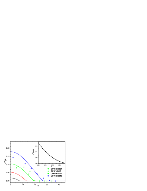
Figure 3: (Color online) The momentum distribution of the pseudogap. The solid line, from top to bottom, is $x=0.05$, $x=0.10$, $x=0.15$, and $x=0.20$, respectively. The symbols are the experimental data of $Bi2212$ (Ref. 26), $Bi2201$ (Ref. 27), and $LSCO$ (Ref. 28). The experimental data are scaled with $t\sim 0.4eV$. Insert is the doping dependence of pseudogap obtained by the linear interpolation of effective parameters.

4. Results in the Superconducting State

To extend our model into the SC state, a phenomenological SC term $-\sum_{k}\Delta_{k}^{SC}\left(d_{k\uparrow}e_{-k\downarrow}+e_{k\uparrow}d_{-k\downarrow}+hc\right)$ is further assumed though the essential mechanism is still unclear now. Here, the SC gap function $\Delta_{k}^{SC}=V\Delta^{SC}\left(\cos k_{x}-\cos k_{y}\right)$ follows the standard d-wave symmetry as evidenced by the ARPES measurementsTKondo ; KTerashima ; Ma ; Wei . $V$ is the pairing potential and $\Delta^{SC}$ denotes the gap parameter which will be determined self-consistently. Clearly, a two-gap scenario is adopted in the SC state. The total gap $\Delta_{k}^{T}$ contains two components: SC gap $\Delta_{k}^{SC}$ and pseudogap $\Delta_{k}^{PG}$. Numerically, the magnitude of $\Delta_{k}^{T}$ is obtained in the same way as $\Delta^{PG}(\theta)$ as discussed in the previous section.

As can be seen from the insert of Fig. 4(a), the magnitude of $\Delta^{SC}(\theta)$ (also SC critical temperature $T_{c}$) increases with increasing doping from $x=0.06$ up to $x=0.25$, where the pseudogap vanishes. It should be pointed out that the magnitude of $\Delta^{SC}(\theta=0)$ is larger than $\Delta^{PG}(\theta=0)$ at about $x=0.15$ at given pairing potential $V=0.23$. These qualitatively agree with the experimental phase diagram. The conventional one-gap slave boson treatment cannot give such doping dependence unless the bosonic condensation is assumedEmery . The suppression of the SC gap is a natural product of the opening of pseudogap. The density of state (DOS) near $E_{f}$ is much reduced as comparing with the normal state. Additionally, this reduction mainly comes from the antinodal region. As well known that they are the main factors to determine the magnitude of d-wave pairing at given pairing potential $V$.

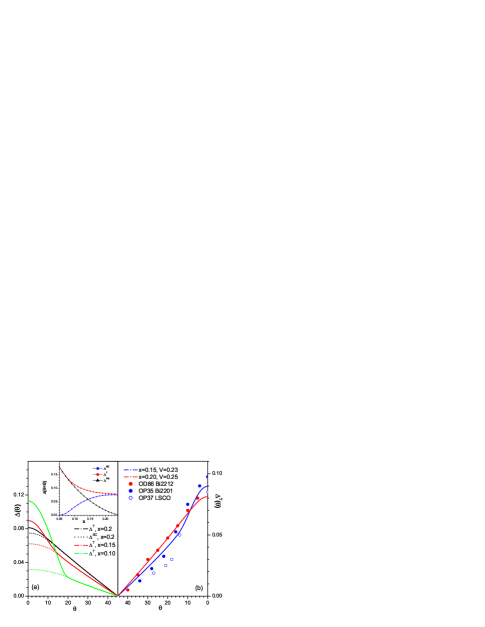
Figure 4: (Color online) (a) The momentum distribution of the total gap in the SC state, together with its corresponding d-wave SC gap with pairing potential $V=0.23$. Insert shows the doping dependence of the total gap $\Delta^{T}$, SC gap $\Delta^{SC}$, and pseudogap $\Delta^{PG}$ at $\theta=0$, the corresponding parameters are obtained by linear interpolation. (b) The comparison of total gap $\Delta^{T}(\theta)$ between the theoretical results and experimental data. Red circles are for $Bi2212$ (Ref. 26), Solid and hollow blue circles are for $Bi2201$ (Ref. 27), and $LSCO$ (Ref. 28), respectively. All experimental data are scaled with $t\sim 0.4eV$

Now, we turn to discuss the momentum distribution of the gap. In the nodal region, $\Delta^{T}(\theta)$ increases almost linearly with decreasing angle $\theta$ as shown in Fig. 4(a). This is the typical d-wave behavior, showing that the d-wave SC pairing dominates this region. In fact, the gap comes from the SC condensation entirely because of the vanished pseudogap along the arc. In the antinodal region, the deviation from the standard d-wave can be found, which weakens upon doping. The shape and value of $\Delta^{T}(\theta=0)$ with small value of $\Delta^{SC}$ are quite similar to that of the pseudogap state, consisting with the so-called ’soft gap’ nature of pseudogapMa . Therefore, the pseudogap dominates the antinodal region. Between the two regions, the pseudogap and the SC gap coexist and compete with each other, so the deviation from the simple d-wave enhances gradually when approaching to the antinodal region. The degree of the deviation depends on the ratio of $\Delta^{SC}\left(\theta=0\right)/\Delta^{PG}(\theta=0)$. Consequently, the deviation weakens upon doping. Such effect can also explain the different deviation in optimal doped $Bi2201$TKondo and $Bi2212$JMesot . These features consist with recent experimentsWSLee ; KTerashima . The deviation had also been obtained in the previous one-gap scenario by applying the spin fluctuation theoryLJX . However, the correction is too small to account for the large deviation in underdoped cuprates. We further compare the experimental data with our theoretical results in Fig. 4 (b). For $Bi2201$TKondo ; Ma and $LSCO$KTerashima materials, a reduced pairing potential $V=0.18$ is adopted. The pseudogap in the two cuprates is almost same as $Bi2212$WSLee at optimal doping, but the SC critical temperature in the former is much weakened than that in the latter. The comparison shows qualitative agreement.

5. Application on Thermodynamic quantities

To justify our theoretical model, the superfluid density $\rho_{s}$ and specific heat $C/T$ are calculated. As well known that $\rho_{s}$ shows almost a low-temperature linear $T$ behavior as shown in Fig. 5(a), expected for clean BCS d-wave superconductor, i.e., $\rho_{s}\left(T\right)$ $=\rho_{s}(0)-bT$. In the underdoped region, $\rho_{s}(0)$ strongly depends on the doping $x$, while the coefficient $b$ is less sensitive to $x$. This can not be understood within a simple BCS d-wave model. On the other hand, it seems that there is a contradiction between the large gap and small superfluid density in the one-gap scenarioBroun ; Hetel . In fact, these curves are slightly concave upward. This upward weakens with doping, and disappears when the pseudogap vanishes in the case of heavy overdoping. The magnitude of $\rho_{s}(0)$ increases with doping in the underdoped region. Our results are similar with that of Ref. 55, in which both the pseudogap and SC gap are fitted from the experimental dataNicol . The results of the specific heat $C/T$ are shown in Fig. 5(b). The jump at critical temperature $T_{c}$, i.e., $\delta C/T$ increases rapidly upon doping, while the entropy $S$ seem to extrapolates to negative value at $T=0$. These main features are consistent with the measurements of Loram et alLoram .

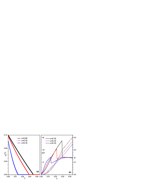
Figure 5: (Color online) (a)Temperature evolution of the superfluid density $\rho_{s}$. (b) Temperature dependence of the specific heat coefficient $C/T$ (left scale) and entropy $S$ (right scale).

6. Conclusion and discussion

In conclusion, we have proposed an effective single particle Hamiltonian to investigate pseudogap in the high-$T_{c}$ cuprates. The dynamic parameters in the Hamiltonian are extracted from the exact diagonalization studies of the $t-J$ model and the consideration of the effective A-B effect. The main idea is to take the effects of two spatial scales into account, one leads to much reduced hopping and the other adds to a phase factor, both reflect physics of the doped holes moving in AFM background. Our results revealed that the pseudogap is the single particle property, and is not directly related to the SC state. It opens near the antinodal region and vanishes around nodal region. In the SC state, the simple d-wave SC gap dominates the nodal region, while the pseudogap dominates the antinodal region. The doping and momentum dependence of the gap are qualitatively consistent with recent ARPES measurements both in the pseudogap state and superconducting state. A two-gap scenario is therefore concluded. The superfluid density and specific heat are further calculated based on the present model, which consists with the experiments qualitatively. Our simple model seems to capture the main features of the underdoped cuprates.

The quasiparticle dispersion obtained from our effective Hamiltonian slightly differs from those obtained by the numerical calculationsNodegap ; Sakai , where the nodal gap above Fermi surface is found. Since only two main effects with different spatial scale are taken into account in present treatment, such deviation is not surprising. However, we would like to point out that the momentum- and doping dependence of the pseudogap and gap in the superconducting state are insensitive to the nodal gap due to the fact that it is well above the Fermi level (about $40\sim 60mev$). On the other hand, as shown in the Fig. 2, the nodal arc length is slightly larger than the experimental resultsKMShen . This can be modified by further considering the random phase approximations. However, we would like to emphasize that this modification does not change the main tendency of the doping dependence and momentum distribution of the gap. In the present treatment, only the influence of pseudogap on the SC gap is considered. The feedback effect of the SC gap to the pseudogap is not considered, which is expected to suppress the spin-spin correlation and will be studied in future.

Y Zhou acknowledges helpful discussions with A Greco , and JX Li. This work was supported by NSFC Projects No. 10804047, 11274276, and A Project Funded by the Priority Academic Program Development of Jiangsu Higher Education Institutions. CD Gong acknowledges 973 Projects No. 2011CB605906. HQ Lin acknowledges RGC Grant of HKSAR, Project No. HKUST3/CRF/09.

References

- (1) T. Timusk, and B. Statt: Rep. Prog. Phys. 62 (1999) 61.
- (2) Ø. Fischer M. Kugler, I. Maggio-Aprile, C. Berthod, and C. Renner: Rev. Mod. Phys. 79 (2007) 353.
- (3) V. J. Emery, and S. A. Kivelson: Nature 374 (1995) 434.
- (4) P. A. Lee: Physica C 317-318 (1999) 194.
- (5) H. Ding, T. Yokoya, J. C. Campuzano, T. Takahashi, M. Randeria, M. R. Norman, T. Mochiku, K. Kadowaki, and J. Giapintzakis: Nature 382 (1996) 51.
- (6) A. G. Loeser, Z.-X. Shen, D. S. Dessau, D. S. Marshall, C. H. Park, P. Fournier, and A. Kapitulnik: Science 273 (1996) 325.
- (7) T. Valla, A. V. Fedorov, Jinho Lee, J. C. Davis, and G. D. Gu: Science 314 (2006) 1914.
- (8) C. Renner, B. Revaz, J.-Y. Genoud, K. Kadowaki, and Ø. Fischer: Phys. Rev. Lett. 80 (1998) 149.
- (9) J. C. Campuzano, H. Ding, M. R. Norman, H. M. Fretwell, M. Randeria, A. Kaminski, J. Mesot, T. Takeuchi, T. Sato, T. Yokoya, T. Takahashi, T. Mochiku, K. Kadowaki, P. Guptasarma, D. G. Hinks, Z. Konstantinovic, Z. Z. Li, and H. Raffy: Phys. Rev. Lett. 83 (1999) 3709.
- (10) D. G. Hawthorn, S. Y. Li, M. Sutherland, E. Boaknin, R. W. Hill, C. Proust, F. Ronning, M. A. Tanatar, J. Paglionea, L. Tailleferb, D. Peets, R.-X. Liang, D. A. Bonn, W. N. Hardy, and N. N. Kolesnikov: Phys. Rev. B 75 (2007) 104518.
- (11) A. P. Kampf and J. R. Schrieffer: Phys. Rev. B 42 (1990) 7967.
- (12) C. Honerkamp and P. A. Lee: Phys. Rev. Lett. 92 (2004) 177002.
- (13) V. J. Emery, S. A. Kivelson, and H. Q. Lin: Phys. Rev. Lett. 64 (1990) 475.
- (14) S. A. Kivelson, I. P. Bindloss, E. Fradkin, V. Oganesyan, J. M. Tranquada, A. Kapitulnik, and C. Howald: Rev. Mod. Phys. 75 (2003) 1201.
- (15) E. G. Moon and S. Sachdev: Phys. Rev. B 80 (2009) 035117.
- (16) A. Greco: Phys. Rev. Lett. 103 (2009) 217001.
- (17) M. E. Simon and C. M. Varma: Phys. Rev. Lett. 89 (2002) 247003.
- (18) K.-Y. Yang, T. M. Rice, and F.-C. Zhang: Phys. Rev. B 73 (2006) 174501.
- (19) A. Kaminski, S. Rosenkranz, H. M. Fretwell, J. C. Campuzano, Z. Li, H. Raffy, W. G. Cullen, H. You, C. G. Olsonk, C. M. Varma, and H. Höchst: Nature 416 (2002) 610.
- (20) M. Hashimoto, R. H. He, K. Tanaka, J. P. Testaud, W. Meevasana, R. G. Moore, D. H. Lu, H. Yao, Y. Yoshida, H. Eisaki, T. P. Devereaux, Z. Hussain, and Z.-X. Shen: Nature Phys. 6 (2010) 417.
- (21) R. H. He, M. Hashimoto, H. Karapetyan, J. D. Koralek, J. P. Hinton, J. P. Testaud, V. Nathan, Y. Yoshida, H. Yao, K. Tanaka, W. Meevasana, R. G. Moore, D. H. Lu, S.-K. Mo, M. Ishikado, H. Eisaki, Z. Hussain, T. P. Devereaux, S. A. Kivelson, J. Orenstein, A. Kapitulnik, and Z.-X Shen: Science 331 (2011) 1579.
- (22) M. Le Tacon, A. Sacuto, A. Georges, G. Kotliar, Y. Gallais, D. Colson, and A. Forget: Nature Phys. 2 (2006) 537.
- (23) O. J. Lipscombe, B. Vignolle, T. G. Perring, C. D. Frost, and S. M. Hayden: Phys. Rev. Lett. 102 (2009) 167002;
- (24) B. Fauqué, Y. Sidis, V. Hinkov, S. Pailhès, C. T. Lin, X. Chaud, and P. Bourges: Phys. Rev. Lett. 96 (2006) 197001.
- (25) K. Tanaka, W. S. Lee, D. H. Lu, A. Fujimori, T. Fujii, Risdiana, I. Terasaki, D. J. Scalapino, T. P. Devereaux, Z. Hussain, and Z.-X. Shen: Science 314 (2006) 1910.
- (26) W. S. Lee, I. M. Vishik, K. Tanaka, D. H. Lu, T. Sasagawa, N. Nagaosa, T. P. Devereaux, Z. Hussain, and Z.-X. Shen: Nature 450 (2007) 81.
- (27) T. Kondo, T. Takeuchi, A. Kaminski, S. Tsuda, and S. Shin: Phys. Rev. Lett. 98 (2007) 267004.
- (28) K. Terashima, H. Matsui, T. Sato, T. Takahashi, M. Kofu, and K. Hirota: Phys. Rev. Lett. 99 (2007) 017003.
- (29) A. Kanigel, M. R. Norman, M. Randeria, U. Chatterjee, S. Souma, A. Kaminski, H. M. Fretwell, S. Rosenkranz, M. Shi, T. Sato, T. Takahashi, Z. Z. Li, H. Raffy, K. Kadowaki, D. Hinks, L. Ozyuzer, and J. C. Campuzano: Nature Phys. 2 (2006) 447.
- (30) A. Kanigel, U. Chatterjee, M. Randeria, M. R. Norman, G. Koren, K. Kadowaki, and J. C. Campuzano: Phys. Rev. Lett. 101 (2008) 137002.
- (31) J. Brinckmann and P. A. Lee: Phys. Rev. Lett. 82 (1999) 2915.
- (32) F. C. Zhang, G. Gros, T. M. Rice and H. Shiba: Supercond. Sci. Technol. 1 (1988) 36.
- (33) J. E. Sonier, M. Ilton, V. Pacradouni, C. V. Kaiser, S. A. Sabok-Sayr, Y. Ando, S. Komiya, W. N. Hardy, D. A. Bonn, R. Liang, and W. A. Atkinson: Phys. Rev. Lett. 101 (2008) 117001.
- (34) The superconducting gap may also be inhomogeneous, for example, C. V. Parker, A. Pushp, A. N. Pasupathy, K. K. Gomes, J. Wen, Z. Xu, S. Ono, G. Gu, and A. Yazdani: Phys. Rev. Lett. 104 (2010) 117001.
- (35) S. E. Sebastian, N. Harrison, C. H Mielke, R.-X. Liang, D. A. Bonn, W. N. Hardy, and G. G. Lonzarich: Phys. Rev. Lett. 103 (2009) 256405.
- (36) P. W. Leung: Phys. Rev. B 73 (2006) 075104.
- (37) D. A. Ivanov, P. A. Lee, and X. G. Wen: Phys. Rev. Lett. 84 (2000) 3958.
- (38) P. W. Leung: Phys. Rev. B 62 (2000) R6112.
- (39) A. B. Harris, T. C. Lubensky, and E. J. Mele: Phys. Rev. B 40 (1989) 2631.
- (40) W. D.Wise, K. Chatterjee, M. C. Boyer, T. Kondo, T. Takeuchi, H. Ikuta, Z. J. Xu, J. S. Wen, G. D. Gu, Y. Y. Wang, and E. W. Hudson: Nature Phys. 5 (2009) 213.
- (41) Q. S. Yuan, T. K. Lee, and C. S. Ting: Phys. Rev. B 71(2005) 134522 .
- (42) D. S. Marshall, D. S. Dessau, A. G. Loeser, C-H. Park, A. Y. Matsuura, J. N. Eckstein, I. Bozovic, P. Fournier, A. Kapitulnik, W. E. Spicer, and Z.-X. Shen: Phys. Rev. Lett. 76 (1996) 4841.
- (43) M. R. Norman, H. Ding, M. Randeria, J. C. Campuzano, T. Yokoya, T. Takeuchik, T. Takahashi, T. Mochiku, K. Kadowaki, P. Guptasarma, and D. G. Hinks: Nature 392 (1998) 157.
- (44) K. M. Shen, F. Ronning, D. H. Lu, F. Baumberger, N. J. C. Ingle, W. S. Lee, W. Meevasana, Y. Kohsaka, M. Azuma, M. Takano, H. Takagi, and Z.-X. Shen: Science 307 (2005) 901.
- (45) J. X. Li, C. Y. Mou, and T. K. Lee: Phys. Rev. B 62 (2000) 640.
- (46) Y. Lubashevsky and A. Keren: Phys. Rev. B 78 (2008) 020505(R).
- (47) H. B. Yang, J. D. Rameau, P. D. Johnson, T. Valla, A. Tsvelik, and G. D. Gu: Nature 456 (2008) 77.
- (48) J. P. F. LeBlanc, J. P. Carbotte and E. J. Nicol: Phys. Rev. B 83 (2011) 184506.
- (49) A. Greco and M. Bejas: Phys. Rev. B 83 (2011) 212503.
- (50) J.-H. Ma, Z.-H. Pan, F. C. Niestemski, M. Neupane, Y.-M. Xu, P. Richard, K. Nakayama, T. Sato, T. Takahashi, H.-Q. Luo, L. Fang, H.-H. Wen, Ziqiang Wang, H. Ding, and V. Madhavan: Phys. Rev. Lett. 101 (2008) 207002.
- (51) J. Wei, Y. Zhang, H. W. Ou, B. P. Xie, D. W. Shen, J. F. Zhao, L. X. Yang, M. Arita, K. Shimada, H. Namatame, M. Taniguchi, Y. Yoshida, H. Eisaki, and D. L. Feng: Phys. Rev. Lett. 101 (2008) 097005.
- (52) J. Mesot, M. R. Norman, H. Ding, M. Randeria, J. C. Campuzano, A. Paramekanti, H. M. Fretwell, A. Kaminski, T. Takeuchi, T. Yokoya, T. Sato, T. Takahashi, T. Mochiku, and K. Kadowaki: Phys. Rev. Lett. 83 (1999) 840.
- (53) D. M. Broun, W. A. Huttema, P. J. Turner, S. Özcan, B. Morgan, Ruixing Liang, W. N. Hardy, and D. A. Bonn: Phys. Rev. Lett. 99 (2007) 237003.
- (54) I. Hetel, T. R. Lemberger, and M. Randeria: Nature Phys. 3 (2007) 700.
- (55) J. P. Carbotte, K. A. G. Fisher, J. P. F. LeBlanc, and E. J. Nicol: Phys. Rev. B 81 (2010) 014522.
- (56) J. W. Loram, J. Luoa, J. R. Coopera, W. Y. Lianga, J. L. Tallon: J. Phys. Chem. Solids 62 (2001) 59.
- (57) T. Tohyama: Phys. Rev. B 70 (2004) 174517.
- (58) S. Sakai, Y. Motome, and M. Imada: Phys. Rev. B 82 (2010) 134505.