Statistical mechanical analysis of a hierarchical random code ensemble in signal processing

Abstract

We study a random code ensemble with a hierarchical structure, which is closely related to the generalized random energy model with discrete energy values. Based on this correspondence, we analyze the hierarchical random code ensemble by using the replica method in two situations: lossy data compression and channel coding. For both the situations, the exponents of large deviation analysis characterizing the performance of the ensemble, the distortion rate of lossy data compression and the error exponent of channel coding in Gallager’s formalism, are accessible by a generating function of the generalized random energy model. We discuss that the transitions of those exponents observed in the preceding work can be interpreted as phase transitions with respect to the replica number. We also show that the replica symmetry breaking plays an essential role in these transitions.

1 Introduction

Signal processing is one of the main topics in information science and gaining much more significance in modern society. In this connection, statistical mechanical approaches to signal processing have been investigated for decades, which have provided various novel viewpoints to information theory [1, 2].

Among various models in information theory, the random code ensemble is known as a fundamental model. This ensemble was introduced by Shannon [3, 4] and found to show the optimal performance in error correction stated in the channel coding theorem investigated by himself. After the original study, Gallager [5] enforced its significance through the perfection of Shannon’s result. In the context of statistical mechanics, this ensemble can be viewed as a fundamental spin-glass model: in certain limits, this corresponds to the random energy model (REM) proposed and rigorously analyzed by Derrida [6, 7]. This relation was first pointed out by Sourlas [8]. His work has been recognized as an epoch-making result followed by numerous works such as [9, 10, 11] about decoding and [12, 13, 14, 15, 16] about performance-achieving code.

As a generalization of the REM, the model with a hierarchical structure, termed the generalized random energy model (GREM), was also proposed and rigorously solved in [17, 18, 19]. The original motivation of the generalization was to clarify the relation of the GREM with the other mean-field spin glass model such as the Sherrington-Kirkpatrick model [20]. In a recent work, Merhav [21] proposed a random code ensemble with a hierarchical structure for performance improvement and argued that such a hierarchical ensemble has a similar structure to the GREM. Based on such a similarity, he investigated two issues by large deviation analysis: distortion in lossy data compression and performance of the Bayesian decoder in channel coding through the binary symmetric channel (BSC). For lossy data compression, he concluded that for higher performance the parameters describing the hierarchical structure should be tuned to a range where the GREM shows the same thermodynamic behavior as the standard REM. He also discussed that the same tuning of hierarchical parameters for optimal performance holds in channel coding. However, for a decisive conclusion more detailed investigations are desired. As a crucial point, in taking the ensemble average for performance evaluation we need to consider quenched average, whereas in his analysis simpler annealed average was adopted although he gave some justifications.

Under the circumstances, we reinvestigate the hierarchical random code ensemble in a more inclusive way by using the replica method, which enables us to evaluate the performance of the code with quenched average. In our recent work [22], we analyzed the GREM by the replica method and found that the multiple-step replica symmetry breaking (RSB) appears at low temperatures in the quenched limit. The quenched and the annealed limits are connected with each other in a region where a replica number is positive. This positive replica region becomes important for the large deviation analysis of the random code ensemble. We analyze this region in detail and see that the similar RSB transitions again appear. They play a crucial role for the transitions of the distortion rate and Gallager’s error exponent [5, 23], which directly concerns the performance of the random code.

The actual analysis is performed on a generalized discrete random energy model (GDREM). This model, where possible values of random energy are discrete unlike the original REM, can be seen as a generalization of the discrete REM in [24, 25, 26]. We apply the replica analysis to the GDREM and obtain the phase diagram for the region of a non-negative replica number. The GDREM is directly mapped to the hierarchical random code ensemble. This mapping enables us to readily interpret the properties of the GDREM in the context of the random code. Phase transitions involving the higher step RSB found in the GDREM are directly connected to those in the distortion rate and Gallager’s error exponent. We emphasize that the transitions in the region of a positive replica number are not merely theoretical matters in the replica analysis, but also have a practical significance in information theory. The physical interpretations of behaviors of the distortion rate and Gallager’s error exponent constitute a part of main results in this paper.

This paper is organized as follows. In section 2, we introduce the GDREM and analyze the phase diagram using the replica method. We show that many phases coexist on the diagram of temperature versus the replica number. In section 3, we briefly review the discussion of distortion in lossy data compression, and compare the result from our replica analysis of the GDREM with [21]. As shown there, the replica analysis enables us to investigate the distortion rate quite readily. The result indicates that the higher step RSB degrades the performance of a general hierarchical code. Error correction by the Bayesian decoder is studied in section 4, where Gallager’s error exponent is rederived from our result. We show that two-parameter optimization probably becomes significant when correlations between codewords exist. We also point out that the concentration of the Gibbs measure can be strongly related to the performance analysis of the Bayesian decoder. The last section is devoted to the conclusion.

2 The GDREM

In this section we introduce and analyze the GDREM. The REM [6, 7] is one of the fundamental models in spin glasses, and in its definition the energy of respective state is taken as random. Derrida and Gardner generalized the REM, termed the GREM, in their subsequent works [17, 18, 19] by incorporating the hierarchical structure in the random energy. In the original work of the REM or the GREM, the probability distribution of the energy is Gaussian, whereas the GDREM dealt with here is the model of discrete random energy. In the following we study the GDREM with the binomial distribution of hierarchical random energy.

2.1 Random variable representation

First we give the definition of the GDREM. We follow the notation for the GREM in our paper [22]. Prepare $K$ hierarchical levels, and for the $\nu$th level $(1\leq\nu\leq K)$ random variables $\epsilon_{\nu}(1),\epsilon_{\nu}(2),\ldots,\epsilon_{\nu}(M_{\nu})$ are assigned. These random variables $\{\epsilon_{\nu}\}$ become the energy components of the $\nu$th hierarchy. The number of independent random variables for the $\nu$th level, $M_{\nu}$, can be factored as

$$M_{\nu}=(\alpha_{1}\cdots\alpha_{\nu})^{N},$$ (1)

where $\alpha_{\nu}^{N}$ is an integer satisfying $1<\alpha_{\nu}^{N}<2^{N}$ and denotes the number of independent random variables $\{\epsilon_{\nu}\}$ belonging to a state in the $(\nu-1)$st level (see figure 1). For the deepest level $\nu=K$, $M_{K}=(\alpha_{1}\cdots\alpha_{K})^{N}=2^{N}$ must be held.

From the random variables, we introduce $2^{N}$ new variables $\{E_{i}\}$, which represent the energy of the system and are defined as

$$E_{i}=\sum_{\nu=1}^{K}\epsilon_{\nu}(\lfloor(i-1)M_{\nu}/2^{N}\rfloor+1)=\sum_{\nu=1}^{K}\epsilon_{\nu}^{(i)},$$ (2)

where $i=1,\ldots,2^{N}$ and $\lfloor x\rfloor$ denotes the floor function indicating the largest integer not exceeding $x$. This structure is depicted in figure 1.

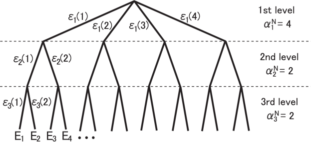
Figure 1: Schematic picture of hierarchical random energy. Here the case of $K=3,N=4$ and $\{\alpha_{1}^{N},\alpha_{2}^{N}\alpha_{3}^{N}\}=\{4,2,2\}$ is depicted. From the root to a leaf (corresponding to a state $i$) of the tree, we sum up $\epsilon_{\nu}(j)$, which becomes the energy of the $i$th state $E_{i}$.

Then, the partition function is defined by

$$Z(\beta)=\sum_{i=1}^{2^{N}}e^{-\beta E_{i}}=\sum_{i=1}^{2^{N}}\exp\left(-\beta\sum_{\nu=1}^{K}\epsilon_{\nu}^{(i)}\right),$$ (3)

with $\beta=1/T$ being the inverse temperature.

The properties of this model are determined by the distribution of the random variables $\{\epsilon_{\nu}\}$. Here we choose the binomial distribution to see the connection with the random code ensemble. For the $\nu$th level, the distribution is characterized by a parameter $L_{\nu}$. The specific form is

$$P_{\nu}(\epsilon_{\nu})=\sum_{l=0}^{L_{\nu}}\frac{L_{\nu}!}{l!(L_{\nu}-l)!}\left(\frac{1}{2}\right)^{L_{\nu}}\delta\left(\epsilon_{\nu},l-\frac{L_{\nu}}{2}\right),$$ (4)

where $\delta(x,y)$ is the Kronecker delta function. The number of possible values of $\epsilon_{\nu}$ is $L_{\nu}+1$, namely, $\epsilon_{\nu}$ can take any of $-L_{\nu}/2,-L_{\nu}/2+1,\ldots,L_{\nu}/2-1,L_{\nu}/2$. For later convenience, we define the parameters $a_{\nu}=L_{\nu}/N$ and $a=\sum_{\nu=1}^{K}a_{\nu}$. In contrast to the case of the Gaussian REM, the value of the parameter $a$ is significant. The RSB occurs only for $a>1$ as discussed in [24], in which case we study in the following.

2.2 Bit representation

Here we give another definition of the GDREM by using bit variables to deal with the hierarchical random code ensemble.

Prepare $aN$ bits taking the value 0 or 1, and divide them into $K$ blocks as $aN=\sum_{\nu=1}^{K}L_{\nu}$. For the $\nu$th block composed of $L_{\nu}$ bits, we randomly choose $M_{\nu}$ bit configurations from possible $2^{L_{\nu}}$ ones, denoted by ${\bm{z}}_{\nu}(1),{\bm{z}}_{\nu}(2),\ldots,{\bm{z}}_{\nu}(M_{\nu})$ where each ${\bm{z}}_{\nu}$ has $L_{\nu}$ components. The $i$th configuration ${\bm{x}}_{i}$ is expressed by arraying the respective configuration of each block as

$$\bm{x}_{i}=\left\{{\bm{z}}_{1}(\lfloor(i-1)M_{1}/2^{N}\rfloor+1),\ldots,{\bm{z}}_{K}(\lfloor(i-1)M_{K}/2^{N}\rfloor+1)\right\},$$ (5)

namely ${\bm{x}}_{i}$ is composed of $aN$ elements. This procedure constructs $2^{N}$ bit configurations from $2^{aN}$ possible ones. The resultant set of chosen configurations, which is denoted as $\cal{C}$ hereafter, has a hierarchy with $K$ levels as the random variable representation.

After construction of states, we define the Hamming distance which counts the number of different bits between bit sequences $\bm{x}_{i}$ and ${\bm{y}}$ as

$$d_{\rm H}(\bm{x}_{i},{\bm{y}})=\sum_{\nu=1}^{K}\sum_{l=1}^{L_{\nu}}\delta({\bm{z}}_{\nu}^{(l)}(\lfloor(i-1)M_{\nu}/2^{N}\rfloor+1),{\bm{y}}_{\nu}^{(l)}).$$ (6)

Here, $\bm{z}_{\nu}^{(l)}$ is the $l$th component of the bit configuration ${\bm{z}}_{\nu}$, and ${\bm{y}}$ is a reference bit sequence which may be chosen as the simplest one such as the all-zero sequence ${\bm{0}}$. Using the Hamming distance, we define the energy of the $i$th state as $E_{i}=d_{\rm H}(\bm{x}_{i},\bm{0})-aN/2$, which leads to the partition function of this system as

$$Z(\beta)=\sum_{{\bm{x}}\in\cal{C}}\exp\left\{-\beta\left(d_{\rm H}({\bm{x}},{\bm{0}})-\frac{aN}{2}\right)\right\}.$$ (7)

The ensemble of bit sequences given here is nothing but the hierarchical random code ensemble introduced in [21]. The energy has the same hierarchical structure as in (2) and the energy of each block is drawn from the binomial distribution in (4), which means that the representation (7) is equivalent to (3). As we see later, this expression is convenient for the discussion of signal processing.

2.3 Replica analysis

We analyze the GDREM by the replica method. As is well known, the replica method is a tool for taking ensemble average of logarithm or arbitrary power of the partition function. This method is thus quite suitable for the performance evaluation of the hierarchical random code ensemble, because the ensemble average of the arbitrary power of the partition function is totally desired, as we see in the following sections. The scheme is the same as demonstrated in [22]. The difference is only in the probability distribution function of energy. We briefly sketch the main result here.

Let us evaluate replicated partition function $Z^{n}$ of the GDREM. When $n$ is a natural number, $Z^{n}$ can be written as

$$Z^{n}(\beta) = \sum_{i_{1}=1}^{2^{N}}\cdots\sum_{i_{n}=1}^{2^{N}}\exp\left(-\beta\sum_{\nu=1}^{K}(\epsilon_{\nu}^{(i_{1})}+\epsilon_{\nu}^{(i_{2})}+\cdots+\epsilon_{\nu}^{(i_{n})})\right)$$ (8)

$$= \sum_{i_{1}=1}^{2^{N}}\cdots\sum_{i_{n}=1}^{2^{N}}\exp\left(-\beta\sum_{\nu=1}^{K}\sum_{j=1}^{M_{\nu}}n_{\nu}(j,\{i_{a}\})\epsilon_{\nu}(j)\right),$$

where

$$n_{\nu}(j,\{i_{a}\})=\sum_{a=1}^{n}I_{\nu}(j,i_{a}),$$ (9)

and $I$ is the indicator function

$$I_{\nu}(j,i_{a})=\left\{\begin{array}[]{cc}1&{\rm for}\ j=\lfloor(i_{a}-1)M_{\nu}/2^{N}\rfloor+1\\ 0&{\rm otherwise.}\end{array}\right.$$ (12)

The ensemble average yields

$$[Z^{n}] = \sum_{i_{1}=1}^{2^{N}}\cdots\sum_{i_{n}=1}^{2^{N}}\exp\left(N\sum_{\nu=1}^{K}\sum_{j=1}^{M_{\nu}}a_{\nu}\ln\cosh\frac{\beta n_{\nu}(j,\{i_{a}\})}{2}\right)$$ (13)

$$= \sum_{\{n_{\nu}\}}\exp\left(S(\{n_{\nu}\})+N\sum_{\nu=1}^{K}\sum_{j=1}^{M_{\nu}}a_{\nu}\ln\cosh\frac{\beta n_{\nu}(j,\{i_{a}\})}{2}\right),$$

where $[\ ]$ means ensemble average and $S(\{n_{\nu}\})$ is the entropy function defined as the logarithm of the number of configurations giving $\{n_{\nu}\}$. In deriving (13), we should take care that the distribution of the energy is binomial, which is only the difference from our preceding work [22]. In the thermodynamic limit $N\to\infty$, we need to calculate the saddle-point contribution of $[Z^{n}]$. A generating function $\phi(\beta,n)\equiv\lim_{N\rightarrow\infty}\ln[Z^{n}]/N$ is convenient for this purpose, and is also significant for signal processing as seen later. In the rest of this section, we focus on calculating this generating function $\phi(\beta,n)$. Hereafter we restrict ourselves to the cases of $K=1,2$ for simplicity.

Practically, we need $\phi(\beta,n)$ for general $n\in\mathbb{R}$, even though the expression (13) is valid only for $n\in\mathbb{N}$. To bridge the gap, we utilize the replica method for analytic continuation from the natural to real number with the Parisi ansatz [27, 28, 29]. For readers not familiar with these procedures, we refer to [1]. Here we demonstrate a part of calculations for the case $K=2$.

According to the standard prescription using the Parisi ansatz, it is sufficient for the current case to consider the replica symmetric (RS) and the one-step RSB (1RSB) solutions in each hierarchy [22, 24]. If the 1RSB occurs in both the hierarchies with different block sizes, it can be interpreted as the two-step RSB (2RSB). Each solution can be graphically expressed by how $n$ “balls” are partitioned into $2^{N}$ “boxes” (figure 2).

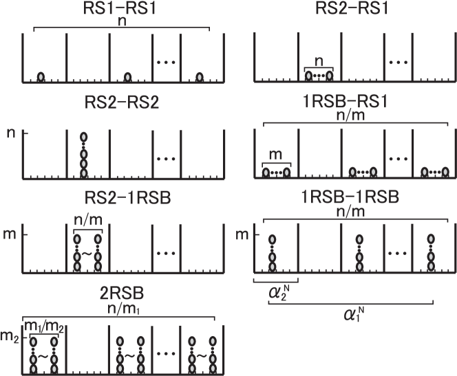
Figure 2: Graphical representation of the possible saddle-point solutions at $K=2$. The horizontal and vertical axes represent the index of configurations and the number of “balls”, respectively. All configurations are divided into $\alpha_{1}^{N}$-groups including $\alpha_{2}^{N}$-configurations.

For each hierarchy, there are two RS solutions: the RS solutions of the first and the second sorts (RS1 and RS2, respectively). For the RS1 solution all $n$ balls are distributed to different states in the hierarchy, while for the RS2 solution all $n$ balls are in the same state in the hierarchy. For example, the RS2-RS1 solution corresponds to the solution being RS2 in the first hierarchy and RS1 in the second one. The entropy of this solution is calculated as

$$S(\{n_{\nu}\})=\ln\{\alpha_{1}^{N}\alpha_{2}^{N}(\alpha_{2}^{N}-1)\cdots(\alpha_{2}^{N}-(n-1))\}\sim N(\ln\alpha_{1}+n\ln\alpha_{2}),$$

and the energetic term becomes

$$\sum_{\nu=1}^{K}\sum_{j=1}^{M_{\nu}}a_{\nu}\ln\cosh\frac{\beta n_{\nu}(j,\{i_{a}\})}{2}=a_{1}\ln\cosh\frac{\beta n}{2}+na_{2}\ln\cosh\frac{\beta}{2}.$$ (15)

These yield the generating function $\phi(\beta,n)$ as

$$\phi(\beta,n)=\ln\alpha_{1}+a_{1}\ln\cosh\frac{\beta n}{2}+n\left(\ln\alpha_{2}+a_{2}\ln\cosh\frac{\beta}{2}\right).$$ (16)

The other solutions are similarly evaluated; therefore, we skip the derivation. For the RSB solutions, there exist additional parameters (such as $m$ and $m_{1,2}$). These parameters are chosen to extremize $\phi(\beta,n)$ and the explicit dependence on those parameters vanishes in the final step. The possible solutions are summarized as follows:

$$\phi(\beta,n)=\left\{\begin{array}[]{ll}n\left(\ln 2+a\ln\cosh\frac{\beta}{2}\right)&{\rm(RS1-RS1)}\\ \ln\alpha_{1}+a_{1}\ln\cosh\frac{\beta n}{2}&\\ \ \ \ \ \ +n\left(\ln\alpha_{2}+a_{2}\ln\cosh\frac{\beta}{2}\right)&{\rm(RS2-RS1)}\\ {\ln 2+a\ln\cosh\frac{\beta n}{2}}&{\rm(RS2-RS2)}\\ {\frac{a_{1}\beta n}{2}\tanh\frac{\beta_{1}}{2}+n\left(\ln\alpha_{2}+a_{2}\ln\cosh\frac{\beta}{2}\right)}&{\rm(1RSB-RS1)}\\ {\ln\alpha_{1}+a_{1}\ln\cosh\frac{\beta n}{2}+\frac{a_{2}\beta n}{2}\tanh\frac{\beta_{2}}{2}}&{\rm(RS2-1RSB)}\\ {\frac{a\beta n}{2}\tanh\frac{\beta_{\rm c}}{2}}&{\rm(1RSB-1RSB)}\\ {\frac{\beta n}{2}\left(a_{1}\tanh\frac{\beta_{1}}{2}+a_{2}\tanh\frac{\beta_{2}}{2}\right)}&{\rm(2RSB)}\\ \end{array}\right.,$$ (25)

where the critical temperature $\beta_{\rm c}$ is defined by the equation

$$R+\ln\cosh\frac{\beta_{\rm c}}{2}-\frac{\beta_{\rm c}}{2}\tanh\frac{\beta_{\rm c}}{2}=0,$$ (27)

with $R\equiv\ln 2/a$. Other critical temperatures $\beta_{1}$ and $\beta_{2}$ are defined by the same equation (27) with substitutions $R=\ln\alpha_{1}/a_{1}\equiv R_{1}$ and $R=\ln\alpha_{2}/a_{2}\equiv R_{2}$, respectively.

Next, we choose the correct solutions from the above seven candidates of $\phi(\beta,n)$, which depend on the values of parameters. We first summarize the case $K=1$ which is naturally included in the above result. For $K=1$, the discrimination between the first and the second hierarchies is useless, which means that the correct solutions are chosen from the RS1-RS1, RS2-RS2 and 1RSB-1RSB solutions (hence abbreviated as RS1, RS2 and 1RSB in the $K=1$ case). When the solution of (27) exists, i.e. $R<\ln 2$ holds, we have three phases on the $T$-$\beta n$ plane as investigated in [24]. The phase diagram in this case is given in figure 3 (left). On the other hand, for the case $\ln 2\leq R$, there is no phase transition and the RS1 solution dominates the whole $T$-$\beta n$ plane, where there is no interest.

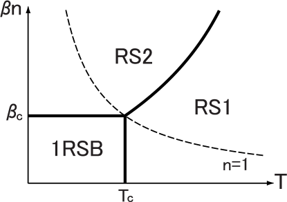
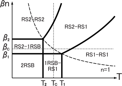
Figure 3: Typical phase diagrams for $K=1$ (left) and $K=2$ with $\ln\alpha_{1}/a_{1}<\ln\alpha_{2}/a_{2}$ and $\beta_{2}<\infty$ (right). $T_{{\rm c},1,2}$ are defined as the inverse of $\beta_{{\rm c},1,2}$ respectively.

In the case of $K=2$, the interesting case is again $R<\ln 2$, i.e. $\beta_{\rm c}$ has a finite value. Moreover, we should distinguish three cases depending on the values of $\beta_{{\rm c},1,2}$.

First, for $R_{2}\leq R_{1}$, the GDREM shows the same behavior as the standard discrete REM, as discussed in [22]. Hence, further investigation is not necessary in this case.

Second, for the case $R_{1}<\ln 2<R_{2}$, where $\beta_{2}$ does not have a finite value, we have three phases: the RS2-RS1, RS1-RS1 and 1RSB-RS1 phases. In this case the second hierarchy is always in the RS1 phase and only the first hierarchy shows phase transitions. In other words the system exhibits a similar phase structure as $K=1$. We focus on the properties of the hierarchical system here, and therefore we skip this case.

The last and the most interesting case is $R_{1}<R_{2}<\ln 2$. This condition means that all the critical temperatures have finite values and $\beta_{1}<\beta_{\rm c}<\beta_{2}$. In this case, there are six phases. The resultant phase diagram is depicted in figure 3 (right). To obtain this phase diagram, we basically determine the contributing phase by the maximization principle based on the saddle-point method. In addition, we need some mathematical and physical criteria such as the continuity of $\phi(\beta,n)$ and the non-negativity of entropy [22]. For instance, let us return to $K=1$ for simplicity. The boundary curve between the RS1 and RS2 phases is obtained by equating $\phi(\beta,n)$ for both the phases. The vertical phase boundary between the RS1 and 1RSB phases is derived by considering entropy crisis, which is identified with spin-glass transition as widely known. The horizontal boundary between the RS2 and 1RSB phases should also exist as described in [24]: the RS2 phase cannot reach the quenched limit $\beta n=0$ because it leads to unphysical behavior, e.g. $\lim_{n\to 0}\phi(\beta,n)/n\to\infty$. Thus, the dominant phase should naturally shift to other phase in decreasing $\beta n$. These discussions can also be applied to $K=2$, where the RSB of multiple step occurs and consequently partial entropy crisis is observed as mentioned in [22].

In the subsequent sections, we move on to the discussions of lossy data compression and channel coding. Actual evaluation of the performance of the random code ensemble is conducted in the range $R_{1}<R_{2}<\ln 2$. The phase diagram (figure 3) and the function $\phi(\beta,n)$ are of great use for this analysis, which explicitly demonstrates the advantage of the replica method.

3 Lossy data compression

We start with the review of lossy data compression in [21]. This issue has also been investigated by statistical mechanics [30, 31, 32, 33], and we concentrate on the hierarchical code here. After establishing how the generating function $\phi(\beta,n)$ relates to lossy data compression, we apply the result of the replica analysis in the previous section.

3.1 Distortion rate

We prepare the hierarchical random code ensemble $\cal C$ with size $2^{N}$ and $aN$-bit hierarchical sequences $(a>1)$ as in [21] or equivalently in section 2.2. For an arbitrary $aN$-bit hierarchical sequence, we represent it by one of the elements in $\cal C$, which amount to the process of lossy data compression. $2^{N}$ sequences out of $2^{aN}$ possible ones have one-to-one correspondence with one of the elements in $\cal C$, whereas others are distorted. To assess the performance of the compression process, we define the distortion (exactly the Hamming distortion) for the signal $\bm{x}$ as

$$\Delta(\bm{x})\equiv\min_{\hat{\bm{x}}\in C}\left(d_{\rm H}(\bm{x},\hat{\bm{x}})-\frac{aN}{2}\right),$$ (28)

where $\bm{x}$ and $\hat{\bm{x}}$ are $aN$-bit sequences. Subtraction of $aN/2$ in the definition is for simplification of the analysis. For extracting more information with regard to the distortion, it is an appropriate manner to define a characteristic function for the distortion [21],

$$\Psi(s)=\left[\exp(-s\Delta({\bm{x}}))\right]_{\bm{x},{\cal C}},$$ (29)

that is, the moment generating function of the distortion. The brackets $[\ ]_{\bm{x},{\cal C}}$ denote the average over $\bm{x}$ and the ensemble of the code. Actually, we may fix the bit sequence $\bm{x}$ as $\bm{x}=\bm{0}$ and remove average over $\bm{x}$, because we take the average over the random code ensemble $[\ ]_{{\cal C}}$. In the large $aN$ limit, the rate of $\Psi(s)$, denoted by $\psi(s)$ and defined as follows, characterizes the performance of the random code ensemble,

$$\psi(s)\equiv-\lim_{N\rightarrow\infty}\frac{\ln\Psi(s)}{aN}=-\lim_{N\rightarrow\infty}\frac{\ln\left[\exp(-s\Delta(\bm{0}))\right]_{\cal C}}{aN}.$$ (30)

This distortion rate $\psi(s)$ has a direct relation with the generating function $\phi(\beta,n)$ of the GDREM. To see this, we should remember that the partition function of the GDREM, $Z(\beta)$, can be written in the bit representation. The distortion $\Delta(0)$ then corresponds to the ground state energy of the GDREM. Accordingly, the following transformation leads to the relation with the replicated partition function of the GDREM:

$$\exp(-s\Delta(\bm{0})) = \lim_{n\rightarrow 0}\left(\sum_{\bm{x}\in{\cal C}}\exp\left\{-\frac{s}{n}\left(d_{\rm H}(\bm{x},\bm{0})-\frac{aN}{2}\right)\right\}\right)^{n}$$ (31)

$$= \lim_{n\rightarrow 0}Z^{n}\left(\frac{s}{n}\right).$$

After taking average over the hierarchical random code ensemble, we have

$$\psi(s)=-\lim_{N\rightarrow\infty}\lim_{n\rightarrow 0}\frac{1}{aN}\ln\left[Z^{n}\left(\frac{s}{n}\right)\right]_{{\cal C}}=-\lim_{n\rightarrow 0}\frac{1}{a}\phi\left(\frac{s}{n},n\right).$$ (32)

Consequently, we can directly assess the distortion rate $\psi(s)$ from the generating function $\phi(\beta,n)$ in the replica analysis.

To summarize, the distortion rate is accessible from the replica analysis using the function $\phi(\beta,n)$ with the constraint $s=\beta n$ and the limit of $n\rightarrow 0$. This means that the contributing phases to $\psi(s)$ are on the $\beta n$ axis in the $T$-$\beta n$ diagram, where there exist phase transitions with respect to $s=\beta n$ as we see in section 2.3. As a result, those transitions lead to the changes of the functional form of the distortion rate.

3.2 Result

In the case of lossy data compression, the parameter $R=\ln 2/a$, which controls the phase transitions of the GDREM, has the significance as the compression rate. Since we deal with compression of data, the compression rate should be smaller than $\ln 2$, in which case the RSB transitions occur as shown in section 2.3.

3.2.1 $K=1$

To calculate the distortion rate $\psi(s)$, we take the limit $n\rightarrow 0$ with keeping $\beta n=s$ in dealing with the function $\phi(\beta,n)$. Accordingly, contributing phases in the current problem turn out to be the RS2 and 1RSB phases. Using (25) and (32), the distortion rate can be derived as

$$\psi(s)=\left\{\begin{array}[]{lll}-\frac{s}{2}\tanh\frac{s_{R}}{2}&({\rm 1RSB})&{\rm for}\ 0\leq s<s_{R}\\ -\ln\cosh\frac{s}{2}-R&({\rm RS2})&{\rm for}\ s_{R}\leq s,\end{array}\right.$$ (35)

where the transition point $s_{R}$ is given from (27),

$$R+\ln\cosh\frac{s_{R}}{2}-\frac{s_{R}}{2}\tanh\frac{s_{R}}{2}=0.$$ (36)

The above solution coincides with the result in [21]. Summarizing, the transition of the distortion rate is interpreted as the phase transition on the $\beta n$ axis in the $T$-$\beta n$ diagram, namely the transition between the RS2 and 1RSB phases.

3.2.2 $K=2$

We consider the case $R_{1}<R_{2}<\ln 2$ as mentioned in section 2.3. As in figure 3, there exist three phases on the $\beta n$ axis, the RS2-RS2, RS2-1RSB and 2RSB. Substituting these solutions into (32), we have

$$\psi(s)=\left\{\begin{array}[]{ll}\frac{s}{2}\left(-\frac{a_{1}}{a}\tanh\frac{s_{R_{1}}}{2}-\frac{a_{2}}{a}\tanh\frac{s_{R_{2}}}{2}\right)&{\rm(2RSB)}\\ &{\rm for}\ 0\leq s<s_{R_{1}}\\ -\frac{a_{1}}{a}\ln\cosh\frac{s}{2}-\frac{a_{1}}{a}R_{1}-\frac{s}{2}\frac{a_{2}}{a}\tanh\frac{s_{R_{2}}}{2}&{\rm(RS2-1RSB)}\\ &{\rm for}\ s_{R_{1}}\leq s<s_{R_{2}}\\ -\ln\cosh\frac{s}{2}-R&{\rm(RS2-RS2)}\\ &{\rm for}\ s_{R_{2}}\leq s,\end{array}\right.$$ (43)

where $s_{R_{1}}$ and $s_{R_{2}}$ are the solutions of equation (36) with substitutions $R=R_{1}$ and $R=R_{2}$, respectively. This also coincides with the result in [21].

3.3 Discussion

To judge whether the hierarchical structure reinforces the performance of the code in lossy data compression or not, we compare the averaged distortion $[\Delta({\bm{0}})]_{\cal C}=\partial\psi/\partial s|_{s=0}$ for both the cases $K=1$ and $2$. The optimal case is the $K=1$ case, because it gives the smallest distortion. This means that the introduction of the hierarchy of the current sort has no positive effect on the lossy data compression, which is the same conclusion as [21]. However, we here stress two advantages of our formulation.

First, our evaluation scheme is quite simple. We can treat both the cases $R_{1}<R_{2}$ and $R_{2}\leq R_{1}$ in a unified framework and can easily see the relation between the cases $K=1$ and $K=2$. Generalization to the larger $K$ cases is also straightforward, whereas such a generalization seems to involve many technical difficulties in the original analysis.

Second, in our approach the transitions observed in the distortion rate can be understood as phase transitions with respect to the replica number, which include the RSB. This can provide more useful insights to signal processing including lossy data compression. For example, we can apply the complexity analysis to the current problem. The complexity, denoted by $\Sigma(E)$ in figure 4, is defined as the logarithm of the number of pure states (see [22, 34] for details), which has a similar meaning to the entropy. Generally speaking, the higher step RSB leads to a decrease in low energy states, which implies the rise in ground-state energy (figure 4).

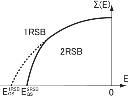
Figure 4: A schematic behavior of complexity as a function of energy. Complexities from the 1RSB and 2RSB solutions are drawn by the dashed and the solid curves, respectively. $E^{\rm 1RSB}_{\rm GS}$ and $E^{\rm 2RSB}_{\rm GS}$ are the ground state energies of the 1RSB and 2RSB phases, respectively. For high energy states both the solutions give the same value of complexity, whereas for low energy states the 2RSB solution yields the smaller one.

This directly elucidates the performance loss of the hierarchical random code ensemble, because the distortion $\Delta(0)$ is identical with the ground-state energy of the GDREM. This observation implies that the higher step RSB generally degrades the performance in lossy data compression.

4 Channel coding

In this section we move on to the problem of channel coding and see the relation with the replica method. Although the basic line of the analysis here is the same as in [24], there is a difference in the discussion of bound for the indicator function.

4.1 General framework

Consider the BSC with reverse probability $p$ $(0\leq p\leq 1/2)$. Following the framework in section 2.2, we also prepare an $N$-bit signal and encode it to a hierarchical $aN$-bit signal ($a>1$), which is included in the codebook $\cal C$ of size $2^{N}$. Then, we transmit an $aN$-bit code sequence $\bm{x}$ through the BSC. The receiver decodes the original signal from an $aN$-bit output by the maximum likelihood decoding, which yields the inferred sequence $\bm{y}$. In the above setting, we define the error probability $P_{\rm E}(\cal C)$ for a given set of original signal and codebook. In particular, we focus on the value averaged over the set of codebook $\cal C$, $\left[P_{\rm E}({\cal C})\right]_{\cal C}$, whose expression is given by

$$\left[P_{\rm E}({\cal C})\right]_{\cal C}=\sum_{\bm{y}}\left[\sum_{\bm{x}\in{\cal C}}P(\bm{x}|{\cal C})P(\bm{y}|\bm{x})\Delta_{\rm ML}(\bm{x},\bm{y}|{\cal C})\right]_{\cal C}.$$ (44)

$P(\bm{x}|\cal C)$ is the prior probability of the original signal $\bm{x}$ and $P(\bm{y}|\bm{x})$ is the posterior probability characterizing the BSC. $\Delta_{\rm ML}(\bm{x},\bm{y}|\cal C)$ is the indicator function of the maximum likelihood decoding, which is zero for successful decoding and unity for failure.

For simplicity, we assume that the probability of the transmit signal $\bm{x}$ is uniform, $P(\bm{x}|{\cal C})=2^{-N}$. The posterior of the BSC is readily calculated as

$$P(\bm{y}|\bm{x}) = (1-p)^{aN-{d_{\rm H}(\bm{x},\bm{y})}}p^{d_{\rm H}(\bm{x},\bm{y})}$$ (45)

$$= \left(\frac{1}{2\cosh(F/2)}\right)^{aN}\exp\left\{-F\left(d_{\rm H}(\bm{x},\bm{y})-\frac{aN}{2}\right)\right\},$$

where $F=\ln\{(1-p)/p\}$ (the Nishimori condition [1, 35]). Besides, we can take the summation over $\bm{y}$ in (44) and replace the reference codeword $\bm{y}$ with $\bm{0}$, because the factor in $\left[~{}\right]_{C}$ becomes independent of $\bm{y}$ due to the summation $\sum_{{\bm{x}}\in{\cal C}}$ and average $\left[~{}\right]_{C}$. Substituting these, we obtain

$$\left[P_{\rm E}({\cal C})\right]_{\cal C}= \frac{1}{2^{N}}\left(\frac{1}{\cosh(F/2)}\right)^{aN}$$ (46)

$$\times\left[\sum_{\bm{x}\in{\cal C}}\exp\left\{-F\left(d_{\rm H}(\bm{x},\bm{0})-\frac{aN}{2}\right)\right\}\Delta_{\rm ML}(\bm{x},\bm{0}|{\cal C})\right]_{\cal C}.$$

It is a formidable task to evaluate the indicator function directly, and its bound is usually discussed by using inequalities. For the hierarchical random code ensemble, it is convenient to use some different inequalities for different $K$.

4.2 Analysis and result

In the case of channel coding, the parameter $R=\ln 2/a$ corresponds to the transmission rate. For successful communication, we have $a>1$ or equivalently $R<\ln 2$, where the RSB phases play significant roles in the GDREM like lossy data compression.

4.2.1 $K=1$

This case corresponds to the conventional random code, and we make use of the inequality in Gallager’s original work [5, 23],

$$\Delta_{\rm ML}(\bm{x},\bm{y}|{\cal C})\leq\left\{\sum_{\tilde{\bm{x}}\in{\cal C}\backslash\bm{x}}\left(\frac{P(\bm{y}|\tilde{\bm{x}})}{P(\bm{y}|\bm{x})}\right)^{\lambda}\right\}^{n}.$$ (47)

The symbol ${\cal C}\backslash\bm{x}$ means the codebook ${\cal C}$ with $\bm{x}$ removed. In this inequality we can take the arbitrary non-negative real values of $\lambda$ and $n$, which should be optimized for the tightest upper bound. In Gallager’s work $\lambda$ was fixed as $\lambda=1/(n+1)$ by using Jensen’s and Hölder’s inequalities. In contrast, in our approach we can readily deal with $\lambda$ without fixing, which is one of the advantageous points of the current analysis. Moreover, the condition $\lambda=1/(n+1)$ may lead to a looser bound in some cases as indicated in [36, 37, 38]. Hence, we adopt the two-parameter optimization here.

Insertion of (45) and (47) into (46) yields

$$\left[P_{\rm E}({\cal C})\right]_{\cal C} \leq \frac{1}{2^{N}}\left(\frac{1}{\cosh(F/2)}\right)^{aN}$$ (48)

$$\times\left[\sum_{\bm{x}\in{\cal C}}\exp\left\{-F(1-n\lambda)\left(d_{\rm H}(\bm{x},\bm{0})-\frac{aN}{2}\right)\right\}\right.$$

$$\times\left.\left(\sum_{\tilde{\bm{x}}\in{\cal C}\backslash\bm{x}}\exp\left\{-F(1-n\lambda)\left(d_{\rm H}(\tilde{\bm{x}},\bm{0})-\frac{aN}{2}\right)\right\}\right)^{n}\right]_{\cal C}.$$

In the current case $K=1$, codewords are not mutually correlated, which allows us to rewrite the upper bound as

$$\left[P_{\rm E}({\cal C})\right]_{\cal C} \leq \frac{1}{2^{N}}\left(\frac{1}{\cosh(F/2)}\right)^{aN}$$

$$\times\left[\sum_{\bm{x}\in{\cal C}}\exp\left\{-F(1-\lambda n)\left(d_{\rm H}(\bm{x},\bm{0})-\frac{aN}{2}\right)\right\}\right]_{\cal C}$$

$$\times\left[\left(\sum_{\tilde{\bm{x}}\in{\cal C}\backslash\bm{x}}\exp\left\{-F\lambda\left(d_{\rm H}(\tilde{\bm{x}},\bm{0})-\frac{aN}{2}\right)\right\}\right)^{n}\right]_{\cal C}$$

$$= \frac{1}{2^{N}}\left(\frac{1}{\cosh(F/2)}\right)^{aN}\exp(N\left\{\phi(F(1-n\lambda),1)+\phi(F\lambda,n)\right\}).$$

With regard to the last factor in the first line, the absence of $\bm{x}$ in the sum over codebook $\cal C$ can be neglected without loss of generality in the limit $N\rightarrow\infty$. Substituting the trivial expression of $\phi(F(1-n\lambda),1)$ and optimizing $\lambda$ and $n$, we obtain the bound

$$\left[P_{\rm E}({\cal C})\right]_{\cal C} \leq \exp(-aNE_{r}^{K=1}(R)),$$ (50)

for $N\rightarrow\infty$, where $E_{r}^{K=1}(R)$ is known as Gallager’s error exponent for the BSC,

$$E_{r}^{K=1}(R)=\mathop{\rm\max}_{0\leq n,\lambda}\left\{-\frac{1}{a}\phi\left(F\lambda,n\right)-\ln\cosh\frac{F(1-\lambda n)}{2}+\ln\cosh\frac{F}{2}\right\}.$$ (51)

Next, we apply the RS1, RS2 and 1RSB solutions in (25) to the computation of the error exponent (51).

• RS1

  The error exponent is expressed as

  $$E_{r}^{K=1}(R) = \mathop{\large\rm max}_{0\leq n,\lambda}\left\{-nR-n\ln\cosh\frac{F\lambda}{2}\right.$$ (52)

  $$\ \ \ \ \ \ \ \left.-\ln\cosh\frac{F(1-\lambda n)}{2}+\ln\cosh\frac{F}{2}\right\}.$$

  From the maximization condition with respect to $n$ we have

  $$R+\ln\cosh\frac{F\lambda}{2}-\frac{F\lambda}{2}\tanh\frac{F\lambda}{2}=0,$$ (53)

  leading $F\lambda=\beta_{\rm c}$. Clearly, this means that the optimal solution is given on the RS1-1RSB boundary if $0\leq n\leq 1$. Hence, we need not to take this solution into account because it can be included in the 1RSB solution. For $n>1$ and $F\lambda=\beta_{\rm c}$, the correct $\phi(F\lambda,n)$ is not given by the RS1, which also leads to the irrelevance of the RS1 solution.

• RS2

  In this case the error exponent is

  $$E_{r}^{K=1}(R) = \mathop{\large\rm max}_{0\leq n,\lambda}\left\{-R-\ln\cosh\frac{F\lambda n}{2}\right.$$ (54)

  $$\ \ \ \ \ \ \ \left.-\ln\cosh\frac{F(1-\lambda n)}{2}+\ln\cosh\frac{F}{2}\right\}.$$

  This form allows us to consider the maximization with respect to the product $\lambda n$, giving $\lambda n=1/2$. The substitution yields

  $$E_{r}^{K=1}(R)=-R-2\ln\cosh\frac{F}{4}+\ln\cosh\frac{F}{2}.$$ (55)

  Due to the functional form of the RS2 solution, where $\lambda$ and $n$ appear only in the product $\lambda n$, we have a redundancy in optimizing $\lambda$ and $n$. On the $T$-$\beta n$ plane, this redundancy means that all the points on a line $\beta n=F/2$ in the RS2 phase give the identical result (55). As $F$ decreases, this horizontal line on the plane goes down along the vertical axis $\beta n$ and finally this reaches the phase boundary between the RS2 and 1RSB phases, which gives the bound of the RS2 solution $2\beta_{\rm c}<F$. This can be regarded as a simple graphical interpretation of the behavior of the error exponent.

• 1RSB

  The error exponent is

  $$E_{r}^{K=1}(R) = \mathop{\large\rm max}_{0\leq n,\lambda}\left\{-\frac{F\lambda n}{2}\tanh\frac{\beta_{\rm c}}{2}-\ln\cosh\frac{F(1-\lambda n)}{2}\right.$$ (56)

  $$\left.\hskip 113.81102pt+\ln\cosh\frac{F}{2}\right\}.$$

  Maximization with respect to $\lambda n$ yields $1-\lambda n=\beta_{\rm c}/F$. Substituting this, we have

  $$E_{r}^{K=1}(R) = -\frac{F}{2}\left(1-\frac{\beta_{\rm c}}{F}\right)\tanh\frac{\beta_{\rm c}}{2}-\ln\cosh\frac{\beta_{\rm c}}{2}+\ln\cosh\frac{F}{2}$$ (57)

  $$= -\frac{F}{2}\tanh\frac{\beta_{\rm c}}{2}+R+\ln\cosh\frac{F}{2}.$$

  Again, on the $T$-$\beta n$ plane, this result is irrespective of temperature similar to the RS2. This solution gives $E_{r}=0$ at $F=\beta_{\rm c}$, which is the bound of successful error correction for the infinite size limit.

Summarizing the above results, we finally obtain

$$E_{r}^{K=1}(R)=\left\{\begin{array}[]{lll}-R-2\ln\cosh\frac{F}{4}&&\\ \qquad+\ln\cosh\frac{F}{2}&{\rm(RS2)}&{\rm for}\ 2\beta_{\rm c}<F\\ -\frac{F-\beta_{\rm c}}{2}\tanh\frac{\beta_{\rm c}}{2}-\ln\cosh\frac{\beta_{\rm c}}{2}&&\\ \qquad+\ln\cosh\frac{F}{2}&{\rm(1RSB)}&{\rm for}\ \beta_{\rm c}\leq F\leq 2\beta_{\rm c}\\ 0&({\rm 1RSB},\beta n=0)&{\rm for}\ F<\beta_{\rm c}.\end{array}\right.$$ (63)

After some calculations, we can confirm that the above error exponent by the replica analysis is in perfect agreement with Gallager’s expression [5, 23], as well as the consistency with Shannon’s channel coding theorem [3, 4].

In fact, the above result is not a novel one, because the error exponent of some models in information theory, including the random code ensemble, has already been investigated by using statistical mechanics in some works [37, 39, 40, 41, 42]. However, the methods used there are different from the one we proposed. We here emphasize some advantages of our method.

The first one is the applicability to larger $K$ cases, which will be demonstrated in the next subsection. In such cases, the codewords are mutually correlated and the analysis becomes more complicated. Despite this, our scheme can evaluate the error exponent without any approximation except for a slight modification of Gallager’s original inequality (47).

Second, as observed and will be observed again for larger $K$, the transition of the error exponent is the RSB between the RS2 and 1RSB phases, which provides a simple interpretation of the function form change of the error exponent. This fact has never been observed or discussed explicitly, which might be due to the condition $\lambda=1/(n+1)$ originated from Jensen’s and Hölder’s inequalities. Moreover, our analysis reveals that the RSB transition with respect to the replica number, which cannot be observed from a thermodynamical quantity after the quenched average, is significant in channel coding. This situation is similar to lossy data compression.

In addition, from the above discussion, we can find that the RS1 phase is excluded from contributing phases, which has a significance in successful decoding. The detail will be argued after the analysis of $K=2$.

4.2.2 $K=2$

In this case, the codewords are mutually correlated, which invalidates the factorization (4.2.1). In such a case, the general form (48) should be directly evaluated, as long as Gallager’s inequality (47) is used. This calculation can actually be done by a novel replica approach, which is somewhat different from the standard one. In this approach, we deal with the factor in $[~{}]_{\cal C}$ in (48) as the partition function of the GDREM with $n+1$ replicas. However, there are two noteworthy points: First, the inverse temperatures are not common to all replicas. One replica out of $n+1$ has the inverse temperature $F(1-n\lambda)$, and others have $F\lambda$. This requires the special treatment of one replica with different temperature in the replica analysis. Second, the correlation between the special one replica and other $n$ replicas exists in this case. As seen in the summation in (48), the special one cannot take the same state as those of other $n$ replicas. Hence, we need to introduce asymmetry between replicas, in addition to the RSB among non-special $n$ replicas. This novel replica method will generally be applicable to any other codes with mutual correlation among codewords, under the situation that Gallager’s inequality is used.

Actually, we applied this novel method to $K=2$ and obtained the bound of the error probability. However this approach requires rather involved calculations. Fortunately we can avoid this novel approach by a slight modification of Gallager’s original inequality. In this paper, we demonstrate this simpler approach in the framework of the ordinary replica analysis of the GDREM for $K=2$. We confirmed that the results from both the schemes coincide with each other.

As stated, we use another inequality for the indicator function here, instead of Gallager’s original inequality (47), as

$$\Delta_{\rm ML}(\{\bm{x}_{1},\bm{x}_{2}(\bm{x}_{1})\},\bm{y}|{\cal C})$$ (65)

$$\leq \ \ \ \left(\sum_{\{\bm{x}_{1},\tilde{\bm{x}}_{2}(\bm{x}_{1})\}\in{\cal C}\backslash\{\bm{x}_{1},\bm{x}_{2}(\bm{x}_{1})\}}\left(\frac{P(\bm{y}|\{\bm{x}_{1},\tilde{\bm{x}}_{2}(\bm{x}_{1})\})}{P(\bm{y}|\{\bm{x}_{1},\bm{x}_{2}(\bm{x}_{1})\})}\right)^{\lambda_{1}}\right)^{n_{1}}$$

$$+\left(\sum_{\{\tilde{\bm{x}}_{1},\tilde{\bm{x}}_{2}(\tilde{\bm{x}}_{1})\}\in{\cal C}\backslash\{\bm{x}_{1},\tilde{\bm{x}}_{2}(\bm{x}_{1})\}}\left(\frac{P(\bm{y}|\{\tilde{\bm{x}}_{1},\tilde{\bm{x}}_{2}(\tilde{\bm{x}}_{1})\})}{P(\bm{y}|\{\bm{x}_{1},\bm{x_{2}}(\bm{x}_{1})\})}\right)^{\lambda_{2}}\right)^{n_{2}},$$

where the codeword $\bm{x}$ is represented by the hierarchical components as $\bm{x}=\{\bm{x}_{1},\bm{x}_{2}(\bm{x}_{1})\}$, and $\{\bm{x}_{1},\tilde{\bm{x}}_{2}(\bm{x}_{1})\}$ is a codeword whose first block is the same as the correct transmission codeword $\bm{x}$. Note that the second-block codeword depends on the first-block one, which is denoted by $\bm{x}_{2}(\bm{x}_{1})$.

Substituting (65) into (46), we can assess the upper bound of the error probability. The contribution from the first term of (65) is equal to

$$\frac{1}{\alpha_{2}^{N}}\left(\frac{1}{\cosh(F/2)}\right)^{a_{2}N}$$

$$\times\left[\sum_{\bm{x}_{2}\in{\cal C}_{2}}\exp\left\{-F(1-\lambda_{1}n_{1})\left(d_{H}(\bm{x}_{2},\bm{0})-\frac{a_{2}N}{2}\right)\right\}\right]_{{\cal C}_{2}}$$

$$\times\left[\ \ \ \left(\sum_{\tilde{\bm{x}}_{2}\in{\cal C}_{2}\backslash\bm{x}_{2}}\exp\left\{-F\lambda_{1}\left(d_{H}(\tilde{\bm{x}_{2}},\bm{0})-\frac{a_{2}N}{2}\right)\right\}\right)^{n_{1}}\right]_{{\cal C}_{2}},$$ (66)

where we express the entire codebook ${\cal C}$ by the hierarchical codebooks as ${\cal C}=({\cal C}_{1},{\cal C}_{2})$, then perform the summations and ensemble average with respect to the first hierarchy, $\sum_{{\bm{x}}_{1}}$ and $[~{}]_{{\cal C}_{1}}$. The sizes of codebooks ${\cal C}_{1}$ and ${\cal C}_{2}$ are $\alpha_{1}^{N}$ and $\alpha_{2}^{N}$, respectively. The statistical independence between two different codebooks in the first hierarchy is essential for deriving expression (66). The absence of correlation between ${\bm{x}}_{2}$ and $\tilde{{\bm{x}}}_{2}\neq{\bm{x}}_{2}$ is necessary as well. From the result of $K=1$, this contribution (66) is simply expressed as $\exp(-a_{2}NE_{r}^{K=1}(R_{2}))$.

The contribution from the second term is

$$\frac{1}{2^{N}}\left(\frac{1}{\cosh(F/2)}\right)^{aN}$$

$$\times\left[\sum_{(\bm{x}_{1},\bm{x}_{2}(\bm{x}_{1}))\in{\cal C}}\exp\left\{-F(1-\lambda_{2}n_{2})\left(d_{H}(\{\bm{x}_{1},\bm{x}_{2}(\bm{x}_{1})\},\bm{0})-\frac{aN}{2}\right)\right\}\right]_{\cal C}$$

$$\times\left[\left(\sum_{\{\tilde{\bm{x}}_{1},\tilde{\bm{x}}_{2}(\tilde{\bm{x}}_{1})\}\atop\in{\cal C}\backslash\{\bm{x}_{1},\tilde{\bm{x}}_{2}(\bm{x}_{1})\}}\exp\left\{-F\lambda_{2}\left(d_{H}(\{\tilde{\bm{x}}_{1},\tilde{\bm{x}}_{2}(\tilde{\bm{x}}_{1})\},\bm{0})-\frac{aN}{2}\right)\right\}\right)^{n_{2}}\right]_{\cal C}.$$

To derive this expression, the absence of correlation between $\bm{x}_{1}$ and $\tilde{\bm{x}}_{1}\neq{\bm{x}}_{1}$ is used in a similar manner. As a result, this contribution is represented by the generating function of the GDREM for $K=2$. Denoting this contribution by $\exp(-aNE_{r}^{K=2}(R,R_{1},R_{2}))$, we can write the exponent as

$$E_{r}^{K=2}(R,R_{1},R_{2}) = \mathop{\rm\max}_{0\leq n,\lambda}\left\{-\frac{1}{a}\phi\left(F\lambda,n\right)-\ln\cosh\frac{F(1-\lambda n)}{2}\right.$$ (68)

$$\left.\hskip 113.81102pt+\ln\cosh\frac{F}{2}\right\}.$$

Note that $\phi(F\lambda,n)$ in (68) is for the $K=2$ case. Hence, the bound of the error probability for $K=2$ is expressed as

$$[P_{E}(E)]_{\cal C}\leq\exp(-a_{2}NE_{r}^{K=1}(R_{2}))+\exp(-aNE_{r}^{K=2}(R,R_{1},R_{2})),$$ (69)

for $N\rightarrow\infty$. Therefore, we must compare the two contributions by computing $E_{r}^{K=1}(R_{2})$ and $E_{r}^{K=2}(R,R_{1},R_{2})$.

Here we give a comment on (69). For $K=2$, an intuitive discussion in [21] suggests the following result

$$[P_{E}(E)]_{\cal C}\leq\exp(-a_{2}NE_{r}^{K=1}(R_{2}))+\exp(-aNE_{r}^{K=1}(R)),$$ (70)

for $N\rightarrow\infty$, which differs from (69). However, as mentioned later, the difference between (69) and (70) is irrelevant because both the bounds are identical for $N\rightarrow\infty$. Despite this irrelevance, we consider that our result is more natural and suggestive. The reason is as follows: In the case of the hierarchical random code ensemble, we can expect that the error probability can be decomposed into failure event from respective hierarchy. Our result (69) based on (65) clearly reflects this feature. In the same way, we can expect the bound of the error probability for general $K$ as

$$[P_{E}(E)]_{\cal C}\leq\sum_{\nu=1}^{K}\exp\left(-\sum_{j=0}^{\nu-1}(a_{K-j})NE_{r}^{K=\nu}\right),$$ (71)

for $N\rightarrow\infty$. This expression should be confirmed in future works.

Next we compute the bound (69) using the result of the replica analysis. The first term has already been estimated in the analysis of $K=1$, and here we evaluate the second term. As stated in section 2.3, the case of $R_{1}(<R)<R_{2}<\ln 2$ is dealt with here. The detail of the analysis is in A. We summarize the main result in the following.

Contributing phases to the error exponent are the RS2-RS2, RS2-1RSB and 2RSB. The error exponent is obtained as

$$E_{r}^{K=2}(R,R_{1},R_{2})$$ (83)

$$= \left\{\begin{array}[]{ll}-R-2\ln\cosh\frac{F}{4}+\ln\cosh\frac{F}{2}&{\rm(RS2-RS2)}\\ &{\rm for}\ 2\beta_{2}<F\\ -\ln\cosh\frac{1}{2}(F-\beta_{x})-\frac{a_{1}}{a}R_{1}&\\ \quad-\frac{a_{1}}{a}\ln\cosh\frac{\beta_{x}}{2}-\frac{a_{2}}{a}\frac{\beta_{x}}{2}\tanh\frac{\beta_{2}}{2}&\\ \quad+\ln\cosh\frac{F}{2}&{\rm(RS2-1RSB)}\\ &{\rm for}\ \beta_{1}+\beta_{y}\leq F<2\beta_{2}\\ -\frac{F-\beta_{y}}{2}\tanh\frac{\beta_{y}}{2}-\ln\cosh\frac{\beta_{y}}{2}&\\ \quad+\ln\cosh\frac{F}{2}&{\rm(2RSB)}\\ &{\rm for}\ \beta_{y}\leq F\leq\beta_{1}+\beta_{y}\\ 0&({\rm 2RSB},\beta n=0)\\ &{\rm for}\ F\leq\beta_{y},\end{array}\right.$$

where $\beta_{x}$ and $\beta_{y}$ are given by

$$a_{1}\tanh\frac{\beta_{x}}{2}+a_{2}\tanh\frac{\beta_{2}}{2}=a\tanh\frac{F-\beta_{x}}{2},$$

$$a_{1}\tanh\frac{\beta_{1}}{2}+a_{2}\tanh\frac{\beta_{2}}{2}=a\tanh\frac{\beta_{y}}{2}.$$ (84)

As a result, only the phases on the $\beta n$ axis contribute to the error exponent similar to lossy data compression. This property will hold for arbitrary $K$, which simplifies the analysis for larger $K$.

Finally we must compare the contributions from the first and the second terms on right hand side of (69). We checked it numerically and concluded that the first term always dominates when $R_{1}<R_{2}<\ln 2$. On the other hand, for $R_{2}\leq R_{1}$, the second term dominates and yields the same result as $K=1$.

4.3 Discussion

Now we are ready to compare the performances of $K=1$ (non-hierarchical) and $K=2$ for $R_{1}<R_{2}<\ln 2$. Comparing the dominant contribution $\exp(-a_{2}NE_{r}^{K=1}(R_{2}))$ for $K=2$ with the non-hierarchical result $\exp(-aNE_{r}^{K=1}(R))$, we found that the error exponent of the non-hierarchical code always surpasses that of the hierarchical code for fixed $N$. Therefore, the hierarchy degrades the performance of decoding for $R_{1}\leq R_{2}$. Although this conclusion is the same as Merhav’s discussion [21], our formulation has crucial advantages in the way of reasoning.

Our approach has never loosened the bound of the error exponent, except for Gallager’s inequality (47). This can be achieved with the aid of the replica method, and furthermore the two-parameter optimization with respect to $\lambda$ and $n$ can be reasonably conducted. In conventional approaches, several inequalities, such as Hölder and Jensen inequalities, are employed as in [21]. However, in such analyses the parameter optimization is usually performed only with respect to $n$, by fixing $\lambda$ as $\lambda=1/(n+1)$. These manipulations do not only loosen the bound of the error exponent but also obscure the origin of transitions of the error exponent. Without such risks, our formulation enables us to analyze the performance of random codes in detail. As a result, some physical significances of the behavior of the error exponent can be extracted as follows.

We know that the contributing phases to the error exponent always include the RS2 phase and/or the 1RSB phase in their hierarchy, and the RS1 phase is excluded. The reason is probably elucidated as follows. In a successful case of decoding, the concentration of the Gibbs measure to a certain input signal is expected to be realized. In the RS2/1RSB phases such concentration actually occurs: for the RS2 a single state is chosen by definition (see figure 2 or [22, 24]) and for the 1RSB the measure concentration occurs due to glassy nature. On the other hand, for the RS1 phase such concentration does not occur or the phase is paramagnetic, which corresponds to an inefficient decoding. Consequently we do not need to consider the RS1 phase for the discussion of optimal decoding. We expect this argument is applicable to a general code ensemble.

The above observation also gives some benefits in the practical analyses of $\phi(\beta,n)$: this function will always be written by the function of the product $\beta n$ for the contributing RS2/1RSB phases. This is due to the measure concentration for successful decoding, in which case the replicated partition function is written with the product $\beta n$. From this discussion, we also conclude that the condition $\lambda=1/(n+1)$ for the one-parameter optimization, which is used in the original discussion [5, 23] and valid there, sometimes yields a looser upper bound than the two-parameter optimization. Actually, if we put $\lambda=1/(n+1)$ in (69), the RS1 phase becomes included in the final solution, and we obtain a looser bound than (83), although it does not contribute to the error probability for $N\rightarrow\infty$ due to the dominance of the first term $\exp(-a_{2}NE_{r}^{K=1}(R_{2}))$ in the current situation. Hence, the one-parameter optimization used in Gallager’s work should be carefully examined. This observation will also be helpful to other problems of channel coding.

5 Conclusion

We investigated the hierarchical random code ensemble by using the direct relation with the GDREM. We sketched how the replica analysis is carried out and is useful for large deviation analysis, namely computations of the distortion rate in lossy data compression and Gallager’s error exponent in channel coding. We provided formulae for these quantities and demonstrated how they are evaluated in the case of two hierarchy levels. For lossy data compression, the distortion rate from the replica analysis is in perfect agreement with [21]. Using our method, we could calculate the distortion rate quite readily, which is one of the advantageous points. We also interpreted the behavior of the distortion rate in terms of the complexity, and found that the emergence of the higher step RSB degrades the performance of data compression. From the relation between the complexity and the RSB transition, this conclusion will hold for a general hierarchical code, which is helpful in designing code. In addition, we obtained the novel result for channel coding. The procedure to compute the upper bound is different from Gallager’s argument. This difference arises from the correlation between codewords in the replica analysis. Our result from the two-parameter optimization seems quite natural because the measure concentration is associated with optimal performance as we discussed.

In both the problems, we argued that the RSB transition with respect to the replica number is significant. Although our analysis is based on the mapping between two fundamental models in signal processing and spin glasses, we expect the application of the proposed method to other ensembles or problems in signal processing. We also hope that the observation in this paper for data compression or channel coding from the viewpoint of the RSB will be of use in other problems. Such an application will be our future work.

Appendix A Error exponent for $K=2$

We evaluate the error exponent in each phase for the case $K=2$ by using (68) and the result of the replica analysis (25).

• RS1-RS1

  This gives the same result as the RS1 of $K=1$.

• RS2-RS1

  From (25),

  $$E_{r}^{K=2}(R,R_{1},R_{2})$$ (85)

  $$= \mathop{\rm max}_{0\leq n,\lambda}\left\{-\left(R_{1}+\frac{a_{1}}{a}\ln\cosh\frac{Fn\lambda}{2}\right)-n\left(R_{2}+\frac{a_{2}}{a}\ln\cosh\frac{F\lambda}{2}\right)\right.$$

  $$\left.-\ln\cosh\frac{F(1-n\lambda)}{2}+\ln\cosh\frac{F}{2}\right\}.$$

  Two extremization conditions give $F\lambda=\beta_{2}$, which means that the extremization region is always on the boundary between the RS2-RS1 and RS2-1RSB phases, and

  $$\frac{a_{1}}{a}\tanh\frac{n\beta_{2}}{2}+\frac{a_{2}}{a}\tanh\frac{\beta_{2}}{2}=\tanh\frac{F-n\beta_{2}}{2}.$$ (86)

  The error exponent is rewritten as

  $$E_{r}^{K=2}(R,R_{1},R_{2})$$ (87)

  $$= -\left(R_{1}+\frac{a_{1}}{a}\ln\cosh\frac{\beta_{2}\hat{n}}{2}\right)-\frac{a_{2}}{a}\frac{\beta_{2}\hat{n}}{2}\tanh\frac{\beta_{2}}{2}$$

  $$-\ln\cosh\frac{F-\beta_{2}\hat{n}}{2}+\ln\cosh\frac{F}{2},$$

  where $\hat{n}$ is the solution of (86). As mentioned, the extremization region is on the phase boundary, and this result can be included in the case of the RS2-1RSB.

• RS2-RS2

  This gives the same result as the RS2 for $K=1$.

• 1RSB-RS1

  From (25),

  $$E_{r}^{K=2}(R,R_{1},R_{2})$$ (88)

  $$= \mathop{\rm max}_{0\leq n,\lambda}\left\{-\frac{a_{1}}{a}\frac{Fn\lambda}{2}\tanh\frac{\beta_{1}}{2}-n\left(R_{2}+\frac{a_{2}}{a}\ln\cosh\frac{F\lambda}{2}\right)\right.$$

  $$\left.-\ln\cosh\frac{F(1-n\lambda)}{2}+\ln\cosh\frac{F}{2}\right\}.$$

  From two extremization conditions we have $F\lambda=\beta_{2}$, which means that the extremization region is always on the boundary between the 1RSB-RS1 and 2RSB phases, and

  $$\frac{a_{1}}{a}\tanh\frac{\beta_{1}}{2}+\frac{a_{2}}{a}\tanh\frac{\beta_{2}}{2}=\tanh\frac{F-n\beta_{2}}{2}.$$ (89)

  Then the error exponent is changed to

  $$E_{r}^{K=2}(R,R_{1},R_{2})$$ (90)

  $$= -\frac{\beta_{2}\hat{n}}{2}\left(\frac{a_{1}}{a}\tanh\frac{\beta_{1}}{2}+\frac{a_{2}}{a}\tanh\frac{\beta_{2}}{2}\right)$$

  $$-\ln\cosh\frac{F-\beta_{2}\hat{n}}{2}+\ln\cosh\frac{F}{2},$$

  where $\hat{n}$ is the solution of (89). As stated, the extremization region is on the phase boundary. This result can be included in the case of the 2RSB.

• RS2-1RSB

  From (25),

  $$E_{r}^{K=2}(R,R_{1},R_{2})$$ (91)

  $$= \mathop{\rm max}_{0\leq n,\lambda}\left\{-\frac{a_{1}}{a}R_{1}-\frac{a_{1}}{a}\ln\cosh\frac{F\lambda n}{2}-\frac{a_{2}}{a}\frac{F\lambda n}{2}\tanh\frac{\beta_{2}}{2}\right.$$

  $$\left.-\ln\cosh\frac{F(1-\lambda n)}{2}+\ln\cosh\frac{F}{2}\right\}.$$

  The extremization condition with respect to $\lambda n$ gives

  $$\frac{a_{1}}{a}\tanh\frac{F\lambda n}{2}+\frac{a_{2}}{a}\tanh\frac{\beta_{2}}{2}=\tanh\frac{F(1-\lambda n)}{2}.$$ (92)

  Substituting the solution of (92), we have a part of solution (83).

• 2RSB

  From (25),

  $$E_{r}^{K=2}(R,R_{1},R_{2})$$ (93)

  $$= \mathop{\rm max}_{0\leq n,\lambda}\left\{-\frac{F\lambda n}{2}\left(\frac{a_{1}}{a}\tanh\frac{\beta_{1}}{2}+\frac{a_{2}}{a}\tanh\frac{\beta_{2}}{2}\right)\right.$$

  $$\left.-\ln\cosh\frac{F(1-\lambda n)}{2}+\ln\cosh\frac{F}{2}\right\}.$$

  From the extremization with respect to $\lambda n$,

  $$\frac{a_{1}}{a}\tanh\frac{\beta_{1}}{2}+\frac{a_{2}}{a}\tanh\frac{\beta_{2}}{2}=\tanh\frac{F(1-\lambda n)}{2}.$$ (94)

  Inserting the solution of (94), we have a part of solution (83).

References

References

- [1] Nishimori H 2001 Statistical Physics of Spin Glasses and Information Processing: An Introduction (Oxford: Oxford University Press)
- [2] Mézard M and Montanari A 2009 Information, Physics, and Computation (Oxford: Oxford University Press)
- [3] Shannon C E 1948 Bell. Syst. Tech. J. 27 379
- [4] Shannon C E 1948 Bell. Syst. Tech. J. 27 623
- [5] Gallager R G 1965 IEEE Trans. Inform. Theory 11 3
- [6] Derrida B 1980 Phys. Rev. Lett.45 79
- [7] Derrida B 1981 Phys. Rev.B 24 2613
- [8] Sourlas N 1989 Nature 339 693
- [9] Rújan P 1993 Phys. Rev. Lett.70 2968
- [10] Sourlas N 1994 Europhys. Lett. 25 159
- [11] Kabashima Y and Saad D 1998 Europhys Lett. 44 668
- [12] Kanter I and Saad D 1999 Phys. Rev. Lett.83 2660
- [13] Vicente R, Saad D and Kabashima Y 1999 Phys. Rev.E 60 5352
- [14] Kabashima Y, Murayama T and Saad D 2000 Phys. Rev. Lett.84 1355
- [15] Montanari A and Sourlas N 2000 Eur. Phys. J. B 18 107
- [16] Montanari A 2000 Eur. Phys. J. B 18 121
- [17] Derrida B 1985 J. Physique lett. 46 L401
- [18] Derrida N and Gardner E 1986 J. Phys. C: Solid State Phys.19 2253
- [19] Derrida N and Gardner E 1986 J. Phys. C: Solid State Phys.19 5783
- [20] Sherrington D and Kirkpatrick S 1975 Phys. Rev. Lett.35 1792
- [21] Merhav N 2009 IEEE Trans. Inform. Theory 55 1250
- [22] Obuchi T, Takahashi K and Takeda K 2010 J. Phys. A: Math. Theor. 43 485004
- [23] Gallager R G 1968 Information theory and Reliable communication (New York: John Wiley & Sons)
- [24] Ogure K and Kabashima Y 2004 Prog. Theor. Phys. 111 661
- [25] Ogure K and Kabashima Y 2009 J. Stat. Mech. P03010
- [26] Ogure K and Kabashima Y 2009 J. Stat. Mech. P05011
- [27] Parisi G 1980 J. Phys. A: Math. Gen.13 L115
- [28] Parisi G 1980 J. Phys. A: Math. Gen.13 1101
- [29] Pasiri G 1980 J. Phys. A: Math. Gen.13 1887
- [30] Murayama T 2002 J. Phys. A: Math. Gen.35 L95
- [31] Hosaka T, Kabashima Y and Nishimori H 2002 Phys. Rev.E 66 066126
- [32] Murayama T and Okada M 2003 J. Phys. A: Math. Gen.36 11123
- [33] Hosaka T and Kabashima Y 2005 J. Phys. Soc. Japan 74 488
- [34] Monasson R 1995 Phys. Rev. Lett.75 2847
- [35] Nishimori H 1981 Prog. Theor. Phys. 69 1169
- [36] Aji S, Jin H, Khandekar A, MacKay D J C and McEliece R J 2001 Codes, Systems, and Graphical Models (New York: Springer-Verlag) p 195
- [37] Kabashima Y and Saad D 2004 J. Phys. A: Math. Gen.37 R1
- [38] Hayashi M 2006 Quantum Information: An Introduction (Berlin: Springer-Verlag)
- [39] Kabashima Y, Sazuka N, Nakamura K and Saad D 2001 Phys. Rev.E 64 046113
- [40] Montanari A 2001 Eur. Phys. J. B 23 121
- [41] Skantzos N S, van Mourik J, Saad D and Kabashima Y 2003 J. Phys. A: Math. Gen.36 11131
- [42] Mora T and Rivoire O 2006 Phys. Rev.E 74 056110