Mapping out the quasi-condensate transition through the 1D-3D dimensional crossover

Abstract

By measuring the density fluctuations in a highly elongated weakly interacting Bose gas, we observe and quantify the transition from the ideal gas to a quasi-condensate regime throughout the dimensional crossover from a purely 1D to an almost 3D gas. We show that that the entire transition region and the dimensional crossover are described surprisingly well by the modified Yang-Yang model. Furthermore, we find that at low temperatures the linear density at the quasi-condensate transition scales according to an interaction-driven scenario of a longitudinally uniform 1D Bose gas, whereas at high temperatures it scales according to the degeneracy-driven critical scenario of transverse condensation of a 3D ideal gas.

Low-dimensional (1D or 2D) systems can have physical properties dramatically different to their 3D counterparts. Experimental realizations of such systems in recent years have been particularly exciting in the field of ultracold atomic gases PetrovReview ; DalibardBloch . Here the reduction of dimensionality is achieved by using highly anisotropic trapping potentials, in which lowering the temperature leads to “freezing” out certain motional degrees of freedom to the respective ground state. For situations when the “freezing” is not perfect, an intriguing fundamental question arises: How the low-dimensional and the 3D physics get reconciled in the dimensional crossover?

In this paper we address this question for a weakly interacting Bose gas that is confined transversely by a harmonic trap of frequency $\omega_{\perp}/2\pi$, but is homogeneous and is in the thermodynamic limit with respect to the longitudinal direction. The 1D regime is obtained when the thermal energy $k_{B}T$ and the chemical potential $\mu$ become much smaller than the transverse excitation energy $\hbar\omega_{\perp}$. In the absence of interatomic interactions, the homogeneous 1D gas is characterised by the absence of Bose-Einstein condensation. In the 3D limit, however, for $k_{B}T\gg\hbar\omega_{\perp}$, a sharp transverse condensation is expected: the atoms accumulate in the transverse ground state due to the saturation of population in the transversally excited states, yet the resulting 1D gas is still uncondensed with respect to the longitudinal states  . Incorporating weak repulsive interactions, one expects, in the 1D limit, a smooth interaction-driven transition from the ideal gas regime towards the so-called quasi-condensate regime Petrov00 characterized by suppressed density fluctuations while the phase still fluctuates. Quasi-condensates can be also created in the 3D limit Petrov01 , as observed experimentally Quasi-condensate-Hannover ; Quasi-condensate-Orsay . In this paper we investigate the nature of the quasi-condensate transition throughout the whole 1D-3D dimensional crossover.

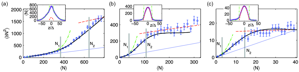
Figure 1: Density fluctuations across the quasi-condensate transition, for $k_{B}T/\hbar\omega_{\perp}=3.6$ (a), 1.0 (b) and 0.09 (c). The measured atom-number variances in individual pixels, $\langle\delta N^{2}\rangle$, as a function of the mean atom number $\langle N\rangle$ are shown as circles, with the error bars representing the statistical uncertainty. Different curves are the predictions from theoretical models, rescaled by the resolution factor $\kappa=0.53$, $0.55$ and $0.4$ for (a), (b) and (c), respectively (see text): modified Yang-Yang model (solid), ideal Bose gas (dash-dotted), quasi-condensate (dashed) and the Poissonian shot-noise level (dotted). The two vertical gray lines give the atom numbers $N_{1}=\Delta n_{1}$ and $N_{2}=\Delta n_{2}$ (see text). The insets show the average density profiles, together with the predictions from the same models (different curves are as in the main graphs). The chemical potential $\mu_{0}$ in the trap center is deduced from the fit of the wings of the density profile to the ideal Bose gas EoS for (a), and from the peak density and the quasi-condensate EoS for (b) and (c). The trap oscillation frequencies are: $\omega_{\perp}/2\pi=3.0$ kHz, $\omega_{\parallel}/2\pi=8.0(5)$ Hz for (a-b) and $\omega_{\perp}/2\pi=3.9$ kHz, $\omega_{\parallel}/2\pi=4.0(5)$ Hz for (c). The absolute temperatures are $T=510$ nK (a), 160 nK (b), and 18 nK (c).

Our study relies on the measurement of atomic density fluctuations, previously used to identify the two limiting regimes – the ideal gas and the quasi-condensate Esteve06 . Owing to a higher measurement precision, we now probe the transition itself, including the crossover from a deeply 1D regime with $k_{B}T\!\ll\!\hbar\omega_{\perp}$ to an almost 3D regime with $k_{B}T\!\simeq\!3\hbar\omega_{\perp}$. For our parameters, the chemical potential becomes non-negligible compared to $\hbar\omega_{\perp}$ only in the quasi-condensate regime so that the dimensional crossover occuring in the quasi-condensate transition is relative to $T$ only. Although the atoms in our experiment are trapped longitudinally, we probe the physics of a longitudinally homogeneous gas because the longitudinal confinement is sufficiently weak and the density fluctuations are measured locally. We find that the transition in the entire dimensional crossover is well described by the so called modified Yang-Yang model (MYYM) Amerongen08 , in which the atoms in the transverse ground state are treated using the exact thermodynamic solution of the 1D Bose gas model with contact interactions YangYang69 , whereas the atoms in the transverse excited states are treated as independent ideal 1D Bose gases. This shows that the quasi-condensate transition maintains its 1D physical origin even for temperatures $k_{B}T\!>\!\hbar\omega_{\perp}$. Moreover, by monitoring the linear density at the quasi-condensation transition, we show that the physics is continuously modified across the dimensional crossover. In the 1D regime, the transition is broad, interaction-driven, and scales as expected from the theory of weakly interacting gases. In the 3D limit, the transition is ruled by the ideal gas scenario of transverse condensation and the transition density no longer depends on the interaction strength. We give a theoretical prediction for the temperature of this dimensional crossover, $T_{DC}$, and show that, unless the interactions are extremely weak, $k_{B}T_{DC}\!\sim\!\hbar\omega_{\perp}$. Dimensional crossover in other ultracold gas systems has been studied both theoretically Das02HardCoreBosons1D-3Dcrossover ; Astrakharchik02QMonteCarlo1D-3D ; Cazalilla04 ; AlKhawaja03dim-Tcrossover and experimentally Gorlitz01 ; Stoferle04Mot1D-3D , but without comparison continuously throughout the crossover.

We conduct our experiment on an atom chip using ⁸⁷Rb atoms in the $|F\!=\!2,m_{F}\!=\!2\rangle$ hyperfine state. The on-chip current carrying micro-wires realise an Ioffe magnetic trap with a longitudinal oscillation frequency ranging from 5.0 Hz to 8 Hz and a transverse oscillation frequency ranging from 3 kHz to 4 kHz. An ultra-cold gas in thermal equilibrium is prepared using rf forced evaporation. We then take in situ absorption images of the atomic cloud using a nearly resonant laser at $\lambda=780$nm, as detailed in ArmijoSkew . The imaging spatial resolution in the object plane has an rms width of about 2 $\mu$m, whereas the camera pixel size is $\Delta=4.5\mu$m. By summing over the transverse pixels, we derive from the images the longitudinal atomic density profile, thus reducing the notion of a pixel to a segment of length $\Delta$. The absolute calibration of the density profiles is described in ArmijoSkew . We perform a statistical analysis of hundreds of images, taken under the same experimental conditions: for each density profile and pixel, we extract the atom number fluctuation $\delta N=N-\langle N\rangle$, where $N$ is the measured number of atoms in the pixel and $\langle N\rangle$ its mean value. The fluctuations are binned according to $\langle N\rangle$ and the variance $\langle\delta N^{2}\rangle$ is computed for each bin. Finally, we subtract the contribution of the optical shot noise, which is typically less than 20% of the atomic fluctuations. Figure 1 shows typical results for $\langle\delta N^{2}\rangle$ for three different temperatures, together with the respective average density profiles. As the images are blurred due to finite imaging resolution, the measured fluctuations are reduced by a factor $\kappa$ compared to their true values. We deduce $\kappa$ from the measurement of atom number correlations between the adjacent pixels, as explained in ArmijoSkew .

For our experimental parameters, we can use the local density approximation along the longitudinal dimension $z$ Kheruntsyan05 , since the correlation length $l_{c}$ of density fluctuations, the pixel length $\Delta$, and the cloud length $L$ satisfy $l_{c}\!\ll\!\Delta\!\ll\!L$. Thus, the gas contained in a pixel $[z,z+\Delta]$ is well described by a longitudinally homogeneous system in the thermodynamic limit, whose local chemical potential is $\mu(z)\!=\!\mu_{0}\!-\!V(z)$, where $V(z)$ is the longitudinal trapping potential. The thermodynamic quantities can be derived from the equation of state (EoS) $n\!=\!n(\mu,T)$ for a longitudinally homogeneous, but transversely trapped gas, where $n$ is the linear (1D) density. In particular, $\langle N\rangle\!=\!n\Delta$ and the atom-number fluctuations can be calculated using the thermodynamic relation

$$\langle\delta N^{2}\rangle=k_{B}T\Delta(\partial n/\partial\mu)_{T}.$$ (1)

Thermometry is done in two alternative ways. For hot gases [such as in Fig. 1 (a)], assuming a perfectly harmonic longitudinal potential, we deduce the temperature by fitting the wings of the density profile to the EoS of an ideal Bose gas,

$$n=\frac{1}{\lambda_{T}}\sum\nolimits_{\alpha=1}^{\infty}\frac{e^{\alpha\mu/k_{B}T}}{\sqrt{\alpha}}\frac{1}{(1-e^{-\alpha\hbar\omega_{\perp}/k_{B}T})^{2}}.$$ (2)

Here, $\lambda_{T}=\sqrt{2\pi\hbar^{2}/mk_{B}T}$ is the thermal de Broglie wavelength, and the EoS is obtained summing the contributions of the transverse harmonic oscillator modes.

For the coldest samples, because of the lack of pixels in the ideal-gas part of the cloud, we deduce the temperature from the measured fluctuations in the quasi-condensate (central) part, using Eq. (1) and the quasi-condensate EoS Fuchs03etMateo2007

$$\mu=\hbar\omega_{\perp}\left(\sqrt{1+4na}-1\right),$$ (3)

valid in the entire 1D-3D crossover region with respect to $\mu$, where $a=5.7~{}$nm is the 3D scattering length. This fluctuation-based thermometry has an accuracy of about $20$%, representing a viable alternative to the thermometry based on the analysis of density ripples appearing after time-of-flight Manz2010 . A related fluctuation-based thermometry Mueller10 ; Sanner10 uses the knowledge of the longitudinal confining potential to deduce the gas compressibility $\partial n/\partial\mu$ from the density profiles. Although less general because of the assumption of validity of Eq. (3), our method has the advantage to work in not perfectly characterised longitudinal potentials, as is often the case in atom-chip experiments Amerongen08 ; Esteve2004 .

Once $\kappa$ and $T$ are determined, the experimental data for the atom number fluctuations are compared with different theoretical models without any further adjustable parameters. As we see from Fig. 1, the two main regimes of a weakly interacting Bose gas KheruntsyanPRL03 ; Kheruntsyan05 are clearly identified. First, at low $\langle N\rangle$ the fluctuations follow the prediction from the ideal gas EoS (2) (dash-dotted curve). Within this regime, but for nondegenerate samples, the fluctuations are Poissonian and follow the shot-noise (dotted) line, as in Fig. 1 (a) for $\langle N\rangle\!<\!200$. For degenerate samples (in the quantum decoherent sub-regime KheruntsyanPRL03 ; Kheruntsyan05 ), atomic bunching due to Bose statistics raises the fluctuations well above the shot-noise level Esteve06 ; BouchouleChipBook . The second main regime is the quasi-condensate regime, where density fluctuations are suppressed by the repulsive interactions. The data in Fig. 1 indeed converge at large $\langle N\rangle$ towards the prediction of the quasi-condensate EoS (3) (dashed lines).

To describe the transition between the two main regimes, we use the modified Yang-Yang model Amerongen08 , whose EoS is

$$n=n_{YY}(\mu,T)+\sum\nolimits_{j=1}^{\infty}(j+1)n_{\rm e}(\mu_{j},T).$$ (4)

Here, the first term describes the atoms in the transverse ground state treated within the exact thermodynamic solution of the 1D Bose gas model YangYang69 , while the second term describes the atoms in the transverse excited states, each treated as an ideal Bose gas with a shifted chemical potential $\mu_{j}=\mu-j\hbar\omega_{\perp}$ and a linear density $n_{\rm e}(\mu_{j},T)=g_{1/2}\left(e^{\mu_{j}/k_{B}T}\right)/\lambda_{T}$, where $g_{1/2}$ is a Bose function. Since $a\ll l_{\perp}$ in our experiment, where $l_{\perp}=\sqrt{\hbar/m\omega_{\perp}}$ is the transverse oscillator length, we use $g=2\hbar\omega_{\perp}a$ Olshanii98 as the effective 1D coupling in the MYYM.

The transition to the quasi-condensate state in a 1D gas occurs when the chemical potential crosses zero Bouchoule07 , over a width $\mu_{t}\!=\!(mg^{2}/\hbar^{2})^{1/3}(k_{B}T)^{2/3}$ BouchouleChipBook . Neglecting correlations between the different transverse states, one can expect the excited state 1D gases to remain nearly ideal and hence the MYYM to correctly describe the quasi-condensate transition as long as $\mu_{t}\!\ll\!\hbar\omega_{\perp}$, or $\mu_{t}/\hbar\omega_{\perp}\!=\!\left[(k_{B}T/\hbar\omega_{\perp})(a/l_{\perp})\right]^{2/3}\!\ll\!1$. Since $a/l_{\perp}\!\simeq 0.03$ in our experiment, the MYYM can be expected to be valid up to temperatures significantly larger than $\hbar\omega_{\perp}/k_{B}$. The experimental data in Fig. 1 are indeed in remarkable agreement with the MYYM prediction in the entire transition region and for all explored temperatures.

In the quasi-condensate regime, however, the MYYM underestimates the fluctuations at high densities. Indeed, when $\mu$ is no longer negligible compared to $\hbar\omega_{\perp}$, the repulsive interactions produce transverse swelling of the density profile – an effect not taken into account in the MYYM. This effect, which is a manifestation of the dimensional crossover with respect to $\mu$ Gorlitz01 , is, on the other hand, captured by the EoS (3), which better describes the quasi-condensate regime [see Fig. 1 (b)].

To quantify the quasi-condensate transition we define the linear densities $n_{1}$ and $n_{2}$ for which the measured fluctuations are 20% lower than the predictions of Eqs. (2) and (3), respectively. Plotting $n_{1}$ and $n_{2}$ against $k_{B}T/\hbar\omega_{\perp}$ (see Fig. 2) maps out the phase diagram and reveals the dimensional crossover as we now explain.

In the 1D limit, $k_{B}T/\hbar\omega_{\perp}\!\ll\!1$, the quasi-condensate transition is expected to occur for a degenerate gas around the density KheruntsyanPRL03 ; Bouchoule07

$$n_{t}\simeq\left[m(k_{B}T)^{2}/\hbar^{2}g\right]^{1/3}.$$ (5)

This estimate can be obtained by considering the EoS of a highly degenerate ideal Bose gas $n\!\simeq\!\sqrt{m(k_{B}T)^{2}/2\hbar^{2}|\mu|}$ , and requiring that $|\mu|$ becomes of the order of the interaction energy $gn$. In the low-temperature (1D) part of the phase diagram, we have fitted the rhs of Eq. (5) to both the $n_{1}$ and $n_{2}$ curves, with two different prefactors $\alpha\!=\!0.28$ and $1.1$, respectively. As we see, the experimental data and the MYYM follow the scaling law of Eq. (5) quite well in this part of the diagram. In contrast, the scaling law of the 1D degeneracy condition, $n_{d}\!=\!1/\lambda_{T}$, does not account for the observed data, which implies that the quasi-condensate transition is governed by interactions and not by degeneracy. Note that the transition begins for a gas that is not highly degenerate, which is a sign that the data are lying close to the crossover towards the strongly interacting regime and which explains why the quantum decoherent sub-regime barely exists in Figs. 1 (b)-(c).

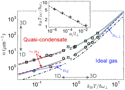
Figure 2: Phase diagram in the 1D-3D crossover. The data at $k_{B}T/\hbar\omega_{\perp}\!<\!0.8$ ($>\!0.8$ kHz) are taken with $\omega_{\perp}/2\pi=3.9$ kHz ($=\!3.0$ kHz). The measured transition boundaries $n_{1}$ (circles) and $n_{2}$ (squares) are plotted along with the predictions from the MYYM (solid gray curves). The dash-dotted curve is the perturbative calculation of $n_{1}$; all other lines are as labeled (see text). The inset shows the dimensional crossover temperature $T_{DC}$ versus $a/l_{\perp}$ (crosses), fitted with a power law $(a/l_{\perp})^{-2/11}$ (dashed line, see text).

In the 3D limit, $k_{B}T/\hbar\omega_{\perp}\!\gg\!1$, $n_{1}$ converges towards the linear density $n_{c\perp}$ corresponding to the the ideal gas scenario of transverse condensation. This occurs when the peak 3D density $\rho_{0}$ reaches the threshold $\rho_{0}\!=\!2.612../\lambda_{T}^{3}$, giving

$$n_{c\perp}=g_{5/2}(1)(k_{B}T/\hbar\omega_{\perp})^{2}/\lambda_{T},$$ (6)

where $g_{5/2}(1)\!=\!1.34..$. For linear densities higher than $n_{c\perp}$, atoms accumulate in the transverse ground state, although no single quantum state is macroscopically occupied. The 3D interaction parameter at the onset of condensation for $T<1~{}\mu$K is $\rho_{0}a^{3}\lesssim 10^{-4}$, so that interactions have a negligible effect in this transition. On the other hand, the ratio $n_{c\perp}/n_{t}$ is of the order of $[(k_{B}T/\hbar\omega_{\perp})(a/l_{\perp})^{2/11}]^{11/6}$. For our experimental parameters, $(l_{\perp}/a)^{2/11}\simeq 1.9$ so that $n_{c\perp}/n_{t}\!\gg\!1$ as soon as $k_{B}T/\hbar\omega_{\perp}\!\gtrsim\!3$. Thus, one expects a quasi-condensate in the transverse ground state to emerge immediately after the transverse condensation. As we see from Fig. 2, Eq. (6) and the MYYM prediction for $n_{1}$ are indeed in very good agreement with each other at high temperatures.

The transition width $(n_{2}-n_{1})/2(n_{1}+n_{2})$ is 0.6 in the 1D regime and decreases as the gas becomes more 3D. Deep in the 3D regime, $n_{2}$ lacks, however, physical meaning. As an example, for our experimental parameters and for $k_{B}T=10\hbar\omega_{\perp}$, one expects only a small fraction of the atoms to be in the quasi-condensate transverse mode at linear density $n_{2}$ and one expects the fluctuations to actually exceed the quasi-condensate prediction at higher densities . We also note that in the 1D limit, the Bogoliubov theory within the quasi-condensate regime Mora03 predicts that the fluctuations are increased slightly when the density is decreased – a feature seen in the MYYM prediction [see Fig. 1 (c)], but which is not resolved experimentally.

In Fig. 2, the change of the scaling of $n_{1}$ from $T^{2/3}$ [Eq. (5)] to $T^{5/2}$ [Eq. (6)] clearly reveals the dimensional crossover. This phase diagram depends, however, on the strength of interactions through the scattering length $a$. To investigate this dependence, we compute $n_{1}$ as a function of $k_{B}T/\hbar\omega_{\perp}$, for several values of $a/l_{\perp}$, using the standard perturbation theory with respect to the 3D coupling $g_{3D}=4\pi\hbar^{2}a/m$, which correctly describes departures from the ideal gas regime. For the parameters of our experiment, with $a/l_{\perp}\!\simeq 0.03$, this calculation (dash-dotted curve in Fig. 2) is in qualitative agreement with the scaling from the 3D to the 1D regime. The disagreement with the data is mainly due to the fact that for such a (large) value of $a/l_{\perp}$, interactions are not negligible even at linear densities smaller than $n_{1}$ . If $a/l_{\perp}$ is decreased, the crossover towards the 3D behavior takes place at a higher temperature. More precisely, $n_{1}$ converges towards $n_{c\perp}$ when $n_{c\perp}\!\gg\!n_{t}$, i.e. when $k_{B}T/\hbar\omega_{\perp}\!\gg\!(a/l_{\perp})^{-2/11}$. By fitting, for each $a/l_{\perp}$, the 1D and 3D asymptotic behavior with the scaling laws of Eqs. (5) and (6), respectively, we define the temperature of the dimensional crossover $T_{DC}$ as the point where these asymptotes intersect. The inset of Fig. 2 shows that $T_{DC}$ scales as $(a/l_{\perp})^{-2/11}$ as expected. We also see that $k_{B}T_{DC}$ becomes significantly larger than $\hbar\omega_{\perp}$ only for extremely small values of $a/l_{\perp}$. In most experimental situations, however, $k_{B}T_{DC}\!\sim\!\hbar\omega_{\perp}$, so that the transverse condensation leads immediately to the formation of a quasi-condensate.

In conclusion, we have mapped out the quasi-condensate transition throughout the 1D-3D dimensional crossover, for $k_{B}T/\hbar\omega_{\perp}$ ranging from $0.06$ to $3.6$. We have found that, whereas the transition is always governed by the 1D physics, it is activated by the degeneracy-driven transverse condensation in the 3D regime while it is interaction driven in the 1D regime. An extension of this work would be to perform similar measurements in 2D gases, characterising the 2D-3D crossover and investigating the breakdown of the scale invariance Rath2010 ; ScaleInvariance2 . For 1D gases, such measurements could also be used to investigate the crossover between the weakly and strongly interacting regimes. More generally, this work shows the power of fluctuation measurements as a test-bed for competing theoretical models for the thermodynamic equation of state of a given physical system.

- (1) D. S. Petrov, D. M. Gangardt, and G. Shlyapnikov, J. Phys. IV (France) 116, 5 (2004).
- (2) I. Bloch, J. Dalibard, and W. Zwerger, Rev. Mod. Phys. 80, 885 (2008), and references therein.
- (3) This phenomenon was first pointed out by N. J. van Druten and W. Ketterle, in Phys. Rev. Lett. 79, 549 (1997), for a system of finite longitudinal size, in which case the atoms eventually condense into the true ground state as the temperature is reduced.
- (4) D. S. Petrov, G. V. Shlyapnikov, and J. T. M. Walraven, Phys. Rev. Lett. 85, 3745 (2000).
- (5) D. S. Petrov, G. V. Shlyapnikov, and J. T. M. Walraven, Phys. Rev. Lett. 87, 050404 (2001).
- (6) S. Dettmer et al., Phys. Rev. Lett. 87, 160406 (2001).
- (7) F. Gerbier et al., Phys. Rev. A 67, 051602 (2003).
- (8) J. Estève et al., Phys. Rev. Lett. 96, 130403 (2006).
- (9) A. H. van Amerongen et al., Phys. Rev. Lett. 100, 090402 (2008).
- (10) C. N. Yang and C. P. Yang, J. Math. Phys. 10, 1115 (1969).
- (11) K. K. Das, M. D. Girardeau, and E. M. Wright, Phys. Rev. Lett. 89, 110402 (2002).
- (12) G. E. Astrakharchik and S. Giorgini, Phys. Rev. A 66, 053614 (2002).
- (13) A. F. Ho, M. A. Cazalilla, and T. Giamarchi, Phys. Rev. Lett. 92, 130405 (2004).
- (14) U. Al Khawaja et al., Phys. Rev. A 68, 043603 (2003).
- (15) A. Görlitz et al., Phys. Rev. Lett. 87, 130402 (2001).
- (16) T. Stöferle et al., Phys. Rev. Lett. 92, 130403 (2004).
- (17) J. Armijo, T. Jacqmin, K. V. Kheruntsyan, and I. Bouchoule, Phys. Rev. Lett. 105, 230402 (2010).
- (18) K. V. Kheruntsyan et al., Phys. Rev. A 71, 053615 (2005).
- (19) J. N. Fuchs, X. Leyronas, and R. Combescot, Phys. Rev. A 68, 043610 (2003), A. Muñoz Mateo and V. Delgado, Phys. Rev. A 77, 013617 (2008).
- (20) S. Manz et al., Phys. Rev. A 81, 031610 (2010).
- (21) T. Müller et al., Phys. Rev. Lett. 105, 040401 (2010).
- (22) C. Sanner et al., Phys. Rev. Lett. 105, 040402 (2010).
- (23) J. Estève et al., Phys. Rev. A 70, 043629 (2004).
- (24) K. V. Kheruntsyan et al., Rev. Lett. 91, 040403 (2003).
- (25) I. Bouchoule, N. J. Van Druten, and C. I. Westbrook, in Atom Chips, Eds. J. Reichel and V. Vuletic (Wiley, Berlin, 2011).
- (26) M. Olshanii, Phys. Rev. Lett. 81, 938 (1998).
- (27) I. Bouchoule, K. V. Kheruntsyan, and G. V. Shlyapnikov, Phys. Rev. A 75, 031606 (2007).
- (28) Eq. (5) and the weak interaction condition give , confirming that the gas is degenerate.
- (29) is obtained from Eq. (2) by taking the limit and then .
- (30) For smaller and/or higher , one can even have .
- (31) C. Mora and Y. Castin, Phys. Rev. A 67, 053615 (2003).
- (32) For smaller values of , the perturbative calculation shows much better agreement with both the scaling law of in the 1D regime and with in the 3D regime.
- (33) S. P. Rath et al., Phys. Rev. A 82, 013609 (2010).
- (34) C.-L. Hung et al., arXiv:1009.0016.