Wave function multifractality and dephasing at metal-insulator and quantum Hall transitions

Abstract

We analyze the critical behavior of the dephasing rate induced by short-range electron-electron interaction near an Anderson transition of metal-insulator or quantum Hall type. The corresponding exponent characterizes the scaling of the transition width with temperature. Assuming no spin degeneracy, the critical behavior can be studied by performing the scaling analysis in the vicinity of the non-interacting fixed point, since the latter is stable with respect to the interaction. We combine an analytical treatment (that includes the identification of operators responsible for dephasing in the formalism of the non-linear sigma-model and the corresponding renormalization-group analysis in $2+\epsilon$ dimensions) with numerical simulations on the Chalker-Coddington network model of the quantum Hall transition. Finally, we discuss the current understanding of the Coulomb interaction case and the available experimental data.

1 Introduction

Localization-delocalization quantum phase transitions form a broad and actively developing field of condensed matter physics, see Ref. [1] for a recent review. In particular, the electron-electron interaction effects at the transition represent one of central research directions [2, 3, 4, 5, 6, 7].

Quite generally, the impact of interaction onto low-temperature transport and localization in disordered electronic systems can be subdivided into effects of (i) renormalization and (ii) dephasing. The renormalization effects, whose role in diffusive systems was investigated by Altshuler and Aronov [2], are governed by virtual processes and become increasingly more pronounced with lowering temperature. Finkelstein developed a renormalization-group (RG) approach [3] in the framework of the non-linear $\sigma$-model in order to treat these effects together with localization phenomena. More recently, this research direction attracted a great deal of attention in connection with experiments on high-mobility low-density electronic structures (Si MOSFETs) giving an evidence in favor of a metal-insulator transition [6, 7, 8]. It was shown that this transition can be explained in the framework of the $\sigma$-model RG for a system with $N>1$ valleys [9] (formally $N$ should be large but in practice $N=2$, as in Si, is already sufficient). Indeed, a detailed analysis has confirmed that the RG theory describes well the experimental data up to lowest accessible temperatures [10, 11]. Very recently, it was shown [12] that interaction effects are also of crucial importance in topological insulators, where they induce novel critical states. Another long-standing issue in the field concerns the interplay of interaction and multifractality of wave functions at Anderson transitions. This problem has been recently addressed in the context of superconductivity near the mobility edge. Focussing on the short-range interaction in the Cooper channel, Ref. [13] predicted that the multifractality of critical wave functions strongly enhances the superconducting pairing correlations.

Dephasing effects are governed by inelastic processes of electron-electron scattering at finite temperature $T$. The dephasing has been studied in great detail for metallic systems where it provides a cutoff for weak-localization effects [2]. As to Anderson localization transitions, dephasing leads to their smearing at finite temperature. The dephasing-induced transition width scales as a power-law function of $T$. In the case of quantum Hall transition, this scaling of the transition width, $\Delta B\propto T^{\kappa}$, has been experimentally explored in many works. While the value of $\kappa$ was a matter of controversy, there seems to be a consensus now that the results $\kappa=0.42\pm 0.04$ [14], $\kappa=0.42\pm 0.01$ [15] properly characterize the quantum Hall transition (when it is not masked by macroscopic inhomogeneities). Scaling near the transition with varying temperature was also experimentally studied at the 3D Anderson transition in doped semiconductors [16, 17].

In this paper we study the scaling properties of dephasing rate at criticality. We consider the situation when the time-reversal invariance is broken, so that the system belongs to the so-called unitary symmetry class. In particular, the quantum Hall transition belongs to this symmetry class. We further assume, following Refs. [18, 19] that the interaction is of short-range character. This greatly simplifies the analysis, since in this case the interaction is irrelevant in the RG sense [4, 18, 20], so that all scaling properties at the transition are governed by the RG flow near the non-interacting fixed point. The goals of this work are as follows. First, we identify the operators controlling the dephasing within the framework of the non-linear $\sigma$-model. Second, we perform the RG analysis of these operators for the $\sigma$-model in $2+\epsilon$ dimensions. Third, we present a numerical investigation of the corresponding wave function correlation functions by using the Chalker-Coddington network as a a model of the quantum Hall transition. Finally, we make conclusions concerning the exponent $\kappa$ governing the temperature scaling of the transition and discuss the current understanding of the Coulomb interaction case, as well as relations between the theoretical and experimental findings.

2 Dephasing rate and exact eigenfunction of the non-interacting problem

2.1 Model

We consider a disordered interacting electronic system characterized by the Hamiltonian

$$\mathcal{H}=\mathcal{H}_{0}+\mathcal{H}_{\rm int}\,.$$ (1)

The one-particle term in the Hamiltonian,

$$\mathcal{H}_{0}=\int d\bm{r}\,\Psi^{{\dagger}}(\bm{r})\Bigl{[}\frac{1}{2m_{e}}(-i\nabla-\bm{A}(\bm{r}))^{2}+V_{\rm dis}(\bm{r})\Bigr{]}\Psi(\bm{r})\,,$$ (2)

is assumed to describe a system with broken time-reversal invariance (unitary symmetry class) at criticality. This may be a 2D system near quantum Hall transition (in which case $\bm{B}={\rm rot}\bm{A}$ is a uniform magnetic field), or a system in $d>2$ dimensions at the Anderson transition point (with a uniform or random magnetic field $\bm{B}(\bm{r})$ breaking the time reversal invariance). The interaction part of the Hamiltonian $\mathcal{H}$ has the form

$$\mathcal{H}_{\textrm{int}}=\,\frac{1}{2}\int d\bm{r_{1}}d\bm{r_{2}}\,U(\bm{r}_{1}-\bm{r}_{2})\Psi^{\dagger}(\bm{r}_{1})\Psi^{\dagger}(\bm{r}_{2})\Psi(\bm{r}_{2})\Psi(\bm{r}_{1})\,,$$ (3)

with a short-range interaction potential $U(r)$.

2.2 First-order correction to the thermodynamic potential

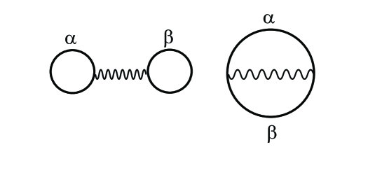
Figure 1: The first-order (Hartree and Fock) interaction corrections to the thermodynamic potential. The wavy line denotes the interaction and the solid line the electron Green’s function.

Following Ref. [18], we begin by considering the first order interaction correction to the thermodynamic potential. The corresponding diagrams are shown in Fig. 1; their total contribution reads

$$\Omega^{(1)}=\frac{1}{2}\sum_{\alpha\beta}n_{f}(\epsilon_{\alpha})n_{f}(\epsilon_{\beta})\int d\bm{r_{1}}d\bm{r_{2}}U(\bm{r_{1}}-\bm{r_{2}})\bigl{|}\mathcal{B}_{\alpha\beta}(\bm{r_{1}},\bm{r_{2}})\bigr{|}^{2}\,,$$ (4)

where $n_{f}(\epsilon)$ is the Fermi-Dirac distribution, $\phi_{\alpha}(\bm{r})$ and $\epsilon_{\alpha}$ are exact eigenfunctions and eigenenergies of the non-interacting Hamiltonian (2), and

$$\mathcal{B}_{\alpha\beta}(\bm{r_{1}},\bm{r_{2}})=\phi_{\alpha}(\bm{r_{1}})\phi_{\beta}(\bm{r_{2}})-\phi_{\alpha}(\bm{r_{2}})\phi_{\beta}(\bm{r_{1}}).$$ (5)

After averaging over disorder, the contribution (4) becomes

$$\langle\Omega^{(1)}\rangle=\int\frac{dEd\omega}{\Delta^{2}}n_{f}(E)n_{f}(E+\omega)\int d\bm{r_{1}}d\bm{r_{2}}U(\bm{r_{1}}-\bm{r_{2}})\mathcal{K}_{1}(\bm{r_{1}},\bm{r_{2}},E,\omega)\,,$$ (6)

where $\Delta=1/\nu_{d}L^{d}$ stands for the mean-level spacing, $L$ is the system size, and $\nu_{d}$ the density of states. The function

$$\mathcal{K}_{1}=\frac{\Delta^{2}}{2}\sum_{\alpha\beta}\left\langle\bigl{|}\mathcal{B}_{\alpha\beta}(\bm{r_{1}},\bm{r_{2}})\bigr{|}^{2}\delta(E+\omega-\epsilon_{\alpha})\delta(E-\epsilon_{\beta})\right\rangle$$ (7)

describes correlations of two eigenstates of the non-interacting Hamiltonian (2). In general, for the system size $L\to\infty$, the function $\mathcal{K}_{1}$ exhibits the following scaling behavior

$$\begin{split}\mathcal{K}_{1}(\bm{r_{1}},\bm{r_{2}},E,\omega)&=L^{-2d}\left(\frac{|\bm{r}_{1}-\bm{r}_{2}|}{L_{\omega}}\right)^{\mu_{2}}\tilde{\mathcal{K}}_{1}\left(\frac{|\bm{r}_{1}-\bm{r}_{2}|}{L_{\omega}}\right),\\ \tilde{\mathcal{K}}_{1}(x)&=\begin{cases}1,\qquad\qquad x\ll 1,\\ x^{-\mu_{2}},\qquad x\gg 1\end{cases}\,,\end{split}$$ (8)

where $L_{\omega}=L(\Delta/|\omega|)^{1/d}$ is the length scale set by the frequency $\omega$. For two adjacent in energy eigenstates one has $\omega\sim\Delta$ and $L_{\omega}\sim L$, for larger frequencies the scale $L_{\omega}$ is much less than $L$. It is important that the exponent $\mu_{2}$ is positive, $\mu_{2}>0$, due to Hartree-Fock antisymmetrization of wave functions in Eq. (5). This means that for distances shorter than $L_{\omega}$ the correlation function (8) is suppressed at criticality as compared to the metallic system. This should be contrasted to multifractal correlations of wave functions (without antisymmetrization) that are enhanced at criticality. We will discuss this point and, more generally, the spectrum of critical exponents within the $\sigma$-model framework in Sec. 3.

We assume the electron-electron interaction of the following form:

$$U(R)=u_{0}\Bigl{[}1+(R/a)^{2}\Bigr{]}^{-\lambda/2}\,,$$ (9)

with $\lambda>d$. This yields

$$\langle\Omega^{(1)}\rangle\propto\int\frac{dEd\omega}{\Delta}n_{f}(E)n_{f}(E+\omega)u(L_{\omega})\,,$$ (10)

where

$$u(L_{\omega})=\nu_{d}u_{0}a^{d}\begin{cases}(a/L_{\omega})^{\mu_{2}},&\qquad d+\mu_{2}<\lambda,\\ (a/L_{\omega})^{\mu_{2}}\ln\frac{L_{\omega}}{a},&\qquad\lambda=d+\mu_{2},\\ (a/L_{\omega})^{\lambda-d},&\qquad d<\lambda<d+\mu_{2}.\end{cases}$$ (11)

Following Ref. [18], we can consider $u(L_{\omega})$ as renormalized interaction parameter. It is seen that for $\lambda>d$ the electron-electron interaction is indeed irrelevant near non-interacting fixed point $u=0$. While the above calculations are based on evaluation of the Hartree-Fock contribution to the thermodynamic potential, this conclusion is in agreement with the analysis of Ref. [20] based on Finkelstein non-linear $\sigma$-model.

2.3 Dephasing rate: Second-order correction to the electron self-energy

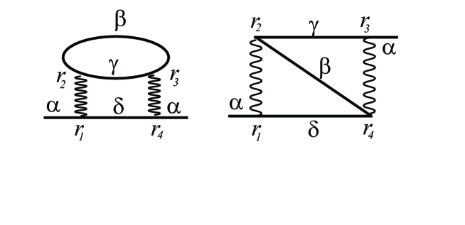
Figure 2: Second-order interaction contributions to the electron self-energy that determine the dephasing rate.

In order to compute the dephasing rate (or, more accurately, the out-scattering rate which in this case coincides with the dephasing rate), one needs to evaluate the second-order interaction correction to the imaginary part of the self-energy (see Fig. 2). In spirit of Ref. [21], we define the self-energy of a given single-particle state $\alpha$,

$$\Sigma_{\alpha}^{R}(\varepsilon)=\frac{1}{8}\int d\bm{r_{1}}d\bm{r_{2}}d\bm{r_{3}}d\bm{r_{4}}U(\bm{r_{1}}-\bm{r_{2}})U(\bm{r_{3}}-\bm{r_{4}})\mathcal{B}^{*}_{\alpha\beta}(\bm{r_{1}},\bm{r_{2}})\mathcal{B}_{\delta\gamma}(\bm{r_{1}},\bm{r_{2}})$$

$$\times\mathcal{B}^{*}_{\gamma\delta}(\bm{r_{3}},\bm{r_{4}})\mathcal{B}_{\beta\alpha}(\bm{r_{3}},\bm{r_{4}})\sum_{\beta\gamma\delta}\frac{n_{f}(\epsilon_{\beta})[1-n_{f}(\epsilon_{\gamma})]+n_{f}(\epsilon_{\delta})[n_{f}(\epsilon_{\gamma})-n_{f}(\epsilon_{\beta})]}{\varepsilon+\epsilon_{\beta}-\epsilon_{\gamma}-\epsilon_{\delta}+i0}.$$ (12)

The next step is the evaluation of the imaginary part of the averaged self-energy

$$\Sigma^{R}(E,\varepsilon)=\Delta\left\langle\sum_{\alpha}\Sigma_{\alpha}^{R}(\varepsilon)\delta(E-\epsilon_{\alpha})\right\rangle.$$ (13)

Since we consider the situation at criticality, where fluctuations may be strong, the averaging is not always an innocent procedure. We will return to the justification of the averaging in Sec. 4.4.

The result of averaging can be presented in the form

$$\operatorname{Im}\Sigma^{R}(E,\varepsilon)=-\pi\left(\prod_{j=1}^{4}\int d\bm{r_{j}}\right)U(\bm{r_{1}}-\bm{r_{2}})U(\bm{r_{3}}-\bm{r_{4}})\int\frac{d\Omega d\varepsilon^{\prime}}{\Delta^{3}}\Bigl{\{}n_{f}(\varepsilon^{\prime}+\Omega)$$

$$\times[1-n_{f}(\varepsilon^{\prime})]+[n_{f}(\varepsilon^{\prime})-n_{f}(\varepsilon^{\prime}+\Omega)]n_{f}(\varepsilon+\Omega)\Bigr{\}}\mathcal{K}_{2}(\{\bm{r}_{j}\},E,\varepsilon,\varepsilon^{\prime},\Omega)\,,$$

where the correlation function $\mathcal{K}_{2}(\{\bm{r}_{j}\},E,\varepsilon,\varepsilon^{\prime},\Omega)$ is defined as follows

$$\mathcal{K}_{2}(\{\bm{r}_{j}\},E,\varepsilon,\varepsilon^{\prime},\Omega)=\frac{\Delta^{4}}{8}\Bigl{\langle}\sum_{\alpha\beta\gamma\delta}\mathcal{B}^{*}_{\alpha\beta}(\bm{r_{1}},\bm{r_{2}})\mathcal{B}_{\delta\gamma}(\bm{r_{1}},\bm{r_{2}})\mathcal{B}^{*}_{\gamma\delta}(\bm{r_{3}},\bm{r_{4}})\mathcal{B}_{\beta\alpha}(\bm{r_{3}},\bm{r_{4}})$$

$$\times\delta(E-\epsilon_{\alpha})\delta(\varepsilon^{\prime}+\Omega-\epsilon_{\beta})\delta(\varepsilon^{\prime}-\epsilon_{\gamma})\delta(\varepsilon+\Omega-\epsilon_{\delta})\Bigr{\rangle}.$$ (15)

To determine the scaling of the dephasing rate, we now specify characteristic values of energy variables. First of all, we are interested in dephasing at the mass shell ($E=\varepsilon$) and at characteristic energy $E\sim T$. Since we are not aiming at calculating the numerical prefactor of order unity, we can simply set $E=0$. Second, we will see that the characteristic values of the integral variables $\varepsilon^{\prime}$ and $\Omega$ are set by the temperature. Performing integration of the Fermi-function factor over energy $\varepsilon^{\prime}$, we find

$$\operatorname{Im}\Sigma^{R}(0,0)\sim-\frac{1}{2\Delta^{3}}\left(\prod_{j=1}^{4}\int d\bm{r_{j}}\right)U(\bm{r_{1}}-\bm{r_{2}})U(\bm{r_{3}}-\bm{r_{4}})\int d\Omega\,\Omega$$

$$\times\Bigl{\{}\coth\frac{\Omega}{2T}-\tanh\frac{\Omega}{2T}\Bigr{\}}\mathcal{K}_{2}(\{\bm{r}_{j}\},0,0,\varepsilon^{\prime}\sim T,\Omega)\,.$$ (16)

In order to proceed further, we need to know the scaling behavior of the function $\mathcal{K}_{2}$. Assuming that $\varepsilon^{\prime}\sim\Omega$ (this is sufficient for our purposes, as both these frequencies are of order of temperature), we have for $|\bm{r}_{1}-\bm{r}_{2}|,|\bm{r}_{3}-\bm{r}_{4}|\ll R\leqslant L_{\Omega}$ the scaling form [18]

$$\mathcal{K}_{2}(\{\bm{r}_{j}\},0,0,\varepsilon^{\prime}\sim\Omega,\Omega)=L^{-4d}\left(\frac{|\bm{r}_{1}-\bm{r}_{2}|}{R}\frac{|\bm{r}_{3}-\bm{r}_{4}|}{R}\right)^{\mu_{2}}\left(\frac{R}{L_{\Omega}}\right)^{\alpha}.$$ (17)

where $\bm{R}=(\bm{r}_{1}+\bm{r}_{2}-\bm{r}_{3}-\bm{r}_{4})/2$. The scaling behavior (17) can be motivated as follows. At distances $R\sim L_{\Omega}$ the correlations between wave functions at $r_{1,2}$, on one hand, and $r_{3,4}$, on the other hand, decouple. Thus, scaling of $\mathcal{K}_{2}$ reduces to that of a product of two independent correlators $\mathcal{K}_{1}$, i.e., $(|\bm{r}_{1}-\bm{r}_{2}|/R)^{\mu_{2}}(|\bm{r}_{3}-\bm{r}_{4}|)/R)^{\mu_{2}}$. The exponent $\alpha$ describes the scaling with respect to a remaining scaling variable $R/L_{\Omega}$. For $R\gg L_{\Omega}$ the correlations quickly (exponentially) decay, so that this range of $R$ is not important for the integral.

Combining Eqs. (16) and (17), we obtain

$$|\operatorname{Im}\Sigma^{R}(0,0)|\sim\nu_{d}T\int_{0}^{T}d\Omega\int_{a}^{L_{\Omega}}d\bm{R}\,u^{2}(R)\left(\frac{R}{L_{\Omega}}\right)^{\alpha}\,.$$ (18)

The result of integration over ${\bf R}$ depends on the relations between $\lambda$, $\mu_{2}$, $\alpha$ and $d$. Let us first assume that $\alpha>-d$. Then, if $\lambda>d+\mu_{2}$, we find

$$\frac{1}{\tau_{\varphi}}\propto\delta u^{2}(a)\begin{cases}(T/\delta)^{1+2\mu_{2}/d},\qquad\qquad d-2\mu_{2}+\alpha>0,\\ (T/\delta)^{1+2\mu_{2}/d}\ln(\delta/T),\quad d-2\mu_{2}+\alpha=0,\\ (T/\delta)^{2+\alpha/d},\qquad\qquad d-2\mu_{2}+\alpha<0.\end{cases}$$ (19)

In the case $\lambda=d+\mu_{2}$, we obtain from Eq. (18)

$$\frac{1}{\tau_{\varphi}}\propto\delta u^{2}(a)\begin{cases}(T/\delta)^{1+2\mu_{2}/d}\ln^{2}(\delta/T),\quad\qquad d-2\mu_{2}+\alpha>0,\\ (T/\delta)^{1+2\mu_{2}/d}\ln^{3}(\delta/T),\qquad d-2\mu_{2}+\alpha=0,\\ (T/\delta)^{2+\alpha/d},\quad\qquad d-2\mu_{2}+\alpha<0.\end{cases}$$ (20)

Finally, if $\lambda<d+\mu_{2}$, we get

$$\frac{1}{\tau_{\varphi}}\propto\delta u^{2}(a)\begin{cases}(T/\delta)^{-1+2\lambda/d},\qquad\qquad 3d-2\lambda+\alpha>0,\\ (T/\delta)^{-1+2\lambda/d}\ln(\delta/T),\quad 3d-2\lambda+\alpha=0,\\ (T/\delta)^{2+\alpha/d},\qquad\qquad 3d-2\lambda+\alpha<0.\end{cases}$$ (21)

Here $\delta=1/\nu_{d}a^{d}$ is the ultraviolet energy cutoff.

For $\alpha\leq-d$, the integration over $\Omega$ is dominated by the infrared cutoff which should be chosen self-consistently at $1/\tau_{\varphi}$, yielding

$$\frac{1}{\tau_{\varphi}}\propto\begin{cases}Tu^{2}(a)|\ln u(a)|,\qquad\qquad\alpha=-d,\\ \delta\left[Tu^{2}(a)/\delta\right]^{-d/\alpha},\qquad\qquad\alpha<-d.\end{cases}$$ (22)

Thus, the temperature behavior of the dephasing rate depends on the exponents $\mu_{2}$ and $\alpha$ as well as on dimensionality $d$ and the index $\lambda$ characterizing the decay of interaction. The exponents $\mu_{2}$ and $\alpha$ belong to a set of exponents characterizing correlations of wave functions at criticality; their values depend on the particular critical point under consideration. In the next section we represent the correlation function $\mathcal{K}_{2}$ in terms of the operators in the non-linear sigma model. This will allow us to substantiate the above scaling arguments by the RG analysis and to evaluate the necessary exponents within the $2+\epsilon$ expansion.

3 Field theoretical approach to wave function correlations

3.1 Non-linear sigma model

The effective theory characterizing long-distance low-energy physics of a disordered electronic system is the non-linear $\sigma$-model [22]. We will use its replica version; the same calculations can be performed in the supersymmetric formulation. The field variable of the theory is the matrix field $Q(\bm{r})$ of size $2n\times 2n$ that obeys the non-linear constraint $Q^{2}(\bm{r})=\bm{1}$. The non-linear sigma model action has the form

$$S_{\sigma}[Q]=-\frac{g}{8}\int d\bm{r}\operatorname{tr}(\nabla Q)^{2}+\frac{gh^{2}}{4}\int d\bm{r}\operatorname{tr}Q\Lambda\,,$$ (23)

where

$$\Lambda=\begin{pmatrix}1_{n}&0\\ 0&-1_{n}\end{pmatrix}.$$ (24)

The parameter $g$ in front of the kinetic term is identified with the dimensionless longitudinal conductance (in units of $e^{2}/h$). In the RG framework, it is interpreted as a running coupling constant of the theory. The second term in Eq. (23), which breaks the ${\rm U}(2n)$ symmetry down to ${\rm U}(n)\times{\rm U}(n)$, normally has an imaginary prefactor proportional to frequency $\varepsilon$. We choose the constant in front of this term to be real, which is more convenient for RG analysis.

In the case of a 2D system in transverse magnetic field, there is an additional contribution to the action that has a form of the topological term  [23]

$$S_{\rm top}[Q]=\frac{\theta}{8\pi}\int d\bm{r}\operatorname{tr}Q\nabla_{x}Q\nabla_{y}Q\,.$$ (25)

The angle $\theta$ in front of the topological term is given by the fractional part of the $2\pi g_{xy}$, where $g_{xy}$ stands for the dimensionless Hall conductivity (in units $e^{2}/h$) [24].

We now proceed by expressing the correlation function $\mathcal{K}_{2}$ in terms of eigenoperators of the $\sigma$-model. This calculation is only based on the symmetry of the theory, so it is equally applicable to the quantum Hall transition in 2D and to the Anderson transition in $d>2$ dimensions.

3.2 Expression for $\mathcal{K}_{2}$ in terms of the eigenoperators

It is convenient to express first the function $\mathcal{K}_{2}$ in terms of the exact single-particle Green’s function $G_{E}^{R,A}(\bm{r},\bm{r}^{\prime})$:

$$\mathcal{K}_{2}(\{\bm{r}_{j}\},E,\varepsilon,\varepsilon^{\prime},\Omega)=\frac{\Delta^{4}}{\pi^{4}}\Bigl{\langle}\operatorname{Im}G_{E}^{R}(\bm{r}_{4},\bm{r}_{1})\operatorname{Im}G_{\varepsilon^{\prime}+\Omega}^{R}(\bm{r}_{3},\bm{r}_{2})\Bigl{[}\operatorname{Im}G_{\varepsilon+\Omega}^{R}(\bm{r}_{1},\bm{r}_{4})$$

$$\times\operatorname{Im}G_{\varepsilon^{\prime}}^{R}(\bm{r}_{2},\bm{r}_{3})-\operatorname{Im}G_{\varepsilon+\Omega}^{R}(\bm{r}_{1},\bm{r}_{3})\operatorname{Im}G_{\varepsilon^{\prime}}^{R}(\bm{r}_{2},\bm{r}_{4})\Bigr{]}\Bigr{\rangle}.$$ (26)

In order to extract the exponent $\alpha$, it is enough to consider scaling of $\mathcal{K}_{2}(\{\bm{r}_{j}\},0,0,0,0)$ with the system size $L$ for fixed $|\bm{r}_{j}-\bm{r}_{k}|$. Then, following standard steps (see e.g. Ref. [25]), we obtain

$$\mathcal{K}_{2}(\{\bm{r}_{j}\},0,0,0,0)=\frac{\Delta^{4}}{(2\pi\gamma)^{4}}\Biggl{\langle}\operatorname{tr}\Bigl{[}\Lambda Q_{ab}(\bm{r_{1}})\Lambda Q_{ba}(\bm{r_{4}})\Bigr{]}\operatorname{tr}\Bigl{[}\Lambda Q_{cd}(\bm{r_{2}})\Lambda Q_{dc}(\bm{r_{3}})\Bigr{]}$$

$$+\operatorname{tr}\Bigl{[}\Lambda Q_{ab}(\bm{r_{1}})\Lambda Q_{bc}(\bm{r_{4}})\Lambda Q_{cd}(\bm{r_{2}})\Lambda Q_{da}(\bm{r_{3}})\Bigr{]}\Biggr{\rangle}$$ (27)

Here $\gamma=(\pi\nu_{d})^{-1}$, the symbol $\operatorname{tr}$ stands for the trace over retarded-advanced space only and $\langle\ldots\rangle$ denotes the averaging with the $\sigma$-model action $S_{\sigma}$. It is important to stress that the replica indices $a,b,c,d$ are fixed and different: $a\neq b\neq c\neq d$. It reflects the fact that we are dealing with four different eigenstates. When deriving Eq. (27), we have assumed that all distances $|\bm{r}_{j}-\bm{r}_{k}|$ exceed the mean free path, so that the averaged Green’s functions between any two points can be neglected. (This assumption does not affect the scaling but simplifies calculations.) On the other hand, we can think about all points as located close to each other from the point of view of the $\sigma$-model (say, on the scale of several mean free paths), so that we omit space argument of $Q$ matrices in what follows.

In view of the presence of the fixed replica indices, Eq. (27) is not convenient for further computations with the action $S_{\sigma}$ which is $U(n)\times U(n)$ invariant. In order to obtain a more convenient, $U(n)\times U(n)$ invariant expression, we use the fact that the correlation function is invariant with respect to global unitary rotations in the replica space. This allows us to average the expression in angular brackets in Eq. (27) over such global unitary rotations. In general, the $U(n)\times U(n)$ invariant operators of the $k$th order in $Q$ matrices have the form $O_{\lambda}=\operatorname{Tr}(\Lambda Q)^{k_{1}}\ldots\operatorname{Tr}(\Lambda Q)^{k_{m}},$ where $\lambda=\{k_{1},\ldots,k_{m}\}$ is a partition of the number $k=k_{1}+\ldots+k_{m}$, such that $k_{1}\geq k_{2}\ldots\geq k_{m}$. In particular, for $k=1$ we have one operator, $\{1\}$, for $k=2$ two operators $\{2\}$ and $\{1,1\}$, for $k=3$ three operators $\{3\}$, $\{2,1\}$, and $\{1,1,1\}$, for $k=4$ five operators $\{4\}$, $\{3,1\}$, $\{2,2\}$, $\{2,1,1\}$, and $\{1,1,1,1\}$, and so on.

Since the correlator $\mathcal{K}_{2}$, Eq. (27), contains four $Q$ matrices, after the averaging over $U(n)\times U(n)$ global rotations the result is expressed in terms of the invariant operators of even orders $\leq 4$, i.e. with $k=4$ and $k=2$ (and in addition a constant term corresponding to $k=0$). Specifically, we obtain (see Appendix B)

$$\mathcal{K}_{2}=\frac{\Delta^{4}}{(2\pi\gamma)^{4}}\left(\sum_{j}C_{j}O_{j}[Q]+C_{0}\right)\,,$$ (28)

where operators $O_{j}[Q]$ and corresponding coefficients are given as

$$O_{4}[Q] = \operatorname{Tr}(\Lambda Q)^{4},$$ (29)

$$O_{3,1}[Q] = \operatorname{Tr}(\Lambda Q)^{3}\operatorname{Tr}\Lambda Q,$$ (30)

$$O_{2,2}[Q] = \operatorname{Tr}(\Lambda Q)^{2}\operatorname{Tr}(\Lambda Q)^{2},$$ (31)

$$O_{2,1,1}[Q] = \operatorname{Tr}(\Lambda Q)^{2}(\operatorname{Tr}\Lambda Q)^{2},$$ (32)

$$O_{1,1,1,1}[Q] = (\operatorname{Tr}\Lambda Q)^{4},$$ (33)

$$O_{2}[Q] = \operatorname{Tr}(\Lambda Q)^{2},$$ (34)

$$O_{1,1}[Q] = (\operatorname{Tr}\Lambda Q)^{2}$$ (35)

and

$$C_{4} = \frac{-3+13n+16n^{2}+4n^{3}}{4n^{2}(-1+n)(1+n)^{2}(2+n)(3+n)},$$ (36)

$$C_{3,1} = -\frac{-7+3n+12n^{2}+4n^{3}}{2n^{2}(-1+n^{2})^{2}(3+n)(2+n)},$$ (37)

$$C_{2,2} = \frac{-3-21n+20n^{2}+32n^{3}+8n^{4}}{8n^{2}(-1+n^{2})^{2}(3+n)(2+n)},$$ (38)

$$C_{2,1,1} = -\frac{3+2n}{2n^{2}(-1+n)(1+n)^{2}(3+n)},$$ (39)

$$C_{1,1,1,1} = \frac{5+5n+2n^{2}}{8n^{2}(-1+n^{2})^{2}(3+n)(2+n)},$$ (40)

$$C_{2} = \frac{-3+3n+4n^{2}}{2n^{2}(-1+n)^{2}(3+n)},$$ (41)

$$C_{1,1} = -\frac{3+5n+4n^{2}}{2n^{2}(-1+n^{2})^{2}(3+n)(2+n)},$$ (42)

$$C_{0} = \frac{-9+93n+4n^{2}-76n^{3}-24n^{4}}{2n(-1+n^{2})^{2}(3+n)(2+n)}.$$ (43)

While the operators $O_{j}[Q]$ are explicitly invariant with respect to the ${\rm U}(n)\times{\rm U}(n)$ symmetry group of the $\sigma$-model, they are not eigenoperators of the renormalization group. The eigenoperators that are linear combinations of $O_{j}[Q]$ are in fact fully determined by the symmetry group (and realize its different representations, similarly to conventional spheric function realizing representations of the rotation group) [29]. The seven RG eigenoperators can be enumerated by Young frames: $P_{4}$, $P_{3,1}$, $P_{2,2}$, $P_{2,1,1}$, $P_{1,1,1,1}$, $P_{2}$, and $P_{1,1}$ [30, 31]. To express these RG eigenoperators in terms of basis operators $O_{j}[Q]$ one can use the results of Refs. [31, 32] or the one-loop renormalization [30, 26]. Finally, using Eq. (28) we represent the correlation function $\mathcal{K}_{2}$ as a linear combination of the eigenoperators of RG,

$$\mathcal{K}_{2}=\frac{\Delta^{4}}{(2\pi\gamma)^{4}}\Biggl{\langle}\frac{4n^{2}}{4n^{2}(n^{2}-1)^{2}}P_{2,2}[Q]-\frac{4n^{2}+8n+3}{6n^{2}(n+1)^{2}(n^{2}+n-2)}P_{2,1,1}[Q]$$

$$+\frac{4n^{2}+16n+15}{2n^{2}(n+1)^{2}(n+2)(n+3)}P_{1,1,1,1}[Q]\Biggr{\rangle}.$$ (44)

It is remarkable that only three eigenoperators (out of seven) enter the obtained expression for the correlation function $\mathcal{K}_{2}$. The eigenoperators $P_{4}$, $P_{3,1}$ and $P_{2}$ with leading singularities in the replica limit $n=0$ do not contribute to $\mathcal{K}_{2}$.

4 Temperature dependence of dephasing rate at criticality

4.1 Anderson transition in $2+\epsilon$ dimensions

In $d=2+\epsilon$ dimensions with small $\epsilon$ the Anderson transition takes place at large dimensionless conductance $g$. This allows one to explore the critical behavior within the $\epsilon$-expansion. The $\beta$-function governing the renormalization of the conductance is known up to the five-loop order [27, 28]

$$-\frac{dt}{d\ln L}=\beta(t)=\epsilon t-2t^{3}-6t^{5}+O(t^{7})\,,$$ (45)

where $t=1/2\pi g$. The metal-insulator transition occurs at the critical point $t_{\star}$ defined by $\beta(t_{\star})=0$ that yields

$$t_{*}=\left(\frac{\epsilon}{2}\right)^{1/2}-\frac{3}{2}\left(\frac{\epsilon}{2}\right)^{3/2}+O(\epsilon^{5/2})\,.$$ (46)

The localization length index $\nu$ reads

$$\nu=-1/\beta^{\prime}(t_{*})=\frac{1}{2\epsilon}-\frac{3}{4}+O(\epsilon)\,.$$ (47)

Further, according to Ref. [31], the anomalous dimensions of the eigenoperators $P_{j}$ are given up to four-loop order as

$$\gamma_{P_{j}}(t)=a_{2}\rho(t)+\zeta(3)c_{3}t^{4}+O(t^{5}),\qquad\rho(t)=t+\frac{3}{2}(n^{2}+1)t^{3}+\frac{n}{3}(n^{2}+7)t^{4}$$ (48)

where coefficients $a_{2}$ and $c_{3}$ are summarized in Table 1. It is worthwhile to mention that the coefficient $c_{3}$ is proportional to $a_{2}$. Therefore, in the replica limit $n\to 0$, the anomalous dimensions of the eigenoperators involved in Eq. (44) become

$$\gamma_{P_{2,2}}(t) = O(t^{5}),$$ (49)

$$\gamma_{P_{2,1,1}}(t) = -4t-6t^{3}+24\zeta(3)t^{4}+O(t^{5}),$$ (50)

$$\gamma_{P_{1,1,1,1}}(t) = -12t-28t^{3}+216\zeta(3)t^{4}+O(t^{5}).$$ (51)

The exponent $\mu_{2}$ is determined by the anomalous dimension of the eigenoperator $P_{1,1}$ [30, 26], see Appendix A. In the replica limit $n\to 0$,

$$\gamma_{P_{1,1}}(t)=-2t-3t^{3}+6\zeta(3)t^{4}+O(t^{5}).$$ (52)

Using Eq. (46), we find the exponent $\mu_{2}$ in $2+\epsilon$ dimensions [26, 31],

$$\mu_{2}=-\gamma_{P_{1,1}}(t_{\star})=\sqrt{2\epsilon}-\frac{3}{2}\zeta(3)\epsilon^{2}+O(\epsilon^{5/2}).$$ (53)

The exponent $\alpha$ is determined by the maximal value of the anomalous dimensions (with oppposite sign) of operators $P_{2,2}$, $P_{2,1,1}$ and $P_{1,1,1,1}$ at the critical point:

$$\alpha=\max\{-\gamma_{P_{2,2}}(t_{\star}),-\gamma_{P_{2,1,1}}(t_{\star}),-\gamma_{P_{1,1,1,1}}(t_{\star})\}.$$ (54)

The anomalous dimensions of the operators $P_{2,1,1}$ and $P_{1,1,1,1}$ are negative, whereas $\gamma_{P_{2,2}}$ vanishes within the known accuracy:

$$\alpha=O(\epsilon^{5/2}).$$ (55)

Table 1: Coefficients of $\gamma$-functions from Ref. [31].

	$a_{2}$	$c_{3}$
$P_{4}$	$12-8n$	$12(3-2n)(2-n)(3-n)$
$P_{3,1}$	$4-8n$	$4(1-2n)(6-13n+n^{2})$
$P_{2,2}$	$-8n$	$84n^{2}$
$P_{2,1,1}$	$-4-8n$	$4(1+2n)(6+13n+n^{2})$
$P_{1,1,1,1}$	$-12-8n$	$12(3+2n)(2+n)(3+n)$
$P_{2}$	$2-4n$	$2(1-2n)(1-n)(3-n)$
$P_{1,1}$	$-2-4n$	$2(1+2n)(1+n)(3+n)$

Therefore, in the case $\lambda>d+\sqrt{2\epsilon}$ (for brevity we keep here only the leading, one-loop, contribution to $\mu_{2}$), the temperature behavior of the dephasing rate is given by

$$\frac{1}{\tau_{\phi}}\propto\delta u^{2}(a)\left(\frac{T}{\delta}\right)^{1+\sqrt{2\epsilon}}.$$ (56)

In the special case $\lambda=d+\sqrt{2\epsilon}$,

$$\frac{1}{\tau_{\varphi}}\propto\delta u^{2}(a)\left(\frac{T}{\delta}\right)^{1+\sqrt{2\epsilon}}\ln^{2}(\delta/T).$$ (57)

Only in the regime $d<\lambda<d+\sqrt{2\epsilon}$, the temperature behavior of the dephasing rate is determined by the exponent $\lambda$:

$$\frac{1}{\tau_{\varphi}}\propto\delta u^{2}(a)\left(\frac{T}{\delta}\right)^{-1+2\lambda/d}.$$ (58)

Let us focus on the case of the “most short-range” interaction, $\lambda>d+\mu_{2}$, when $\tau_{\phi}^{-1}\propto T^{p}$ with $p=1+2\mu_{2}/d$. The scaling of the dephasing length is then given by

$$L_{\phi}\propto T^{-1/z_{T}}\ ;\qquad\qquad z_{T}=\frac{d}{p}=\frac{d}{1+2\mu_{2}/d}\,.$$ (59)

The exponent $z_{T}$ belongs to a class of dynamical critical exponents, as it governs the scaling of a characteristic length scale (dephasing length) with a variable having the dimension of energy. It is worth emphasizing that the localization probems possess rich physics and are in general characterized by several dynamical exponents. This fact has not always been appreciated in the literature. In the present case, one should distinguish the exponent $z_{T}$ controlling the scaling with temperature from the exponent $z$ governing the scaling with frequency. The latter exponent has a trivial (non-interacting) value $z=d$ for the short-range interaction.

The transition width induced by inelastic scattering scales as $T^{\kappa}$, where the exponent $\kappa$ is found by comparison of the dephasing length (59) with the localization (correlation) length $\xi\propto|P-P_{c}|^{-\nu}$, where $P$ is the parameter, driving the transition (e.g., electron concentration or disorder strength). This yields

$$\kappa=\frac{1}{z_{T}\nu}=\frac{1+2\mu_{2}/d}{\nu d}\,.$$ (60)

Substituting the above formulas for $\mu_{2}$ and $\nu$, we get the following results for the dynamical exponent $z_{T}$ and for the index $\kappa$ up to four-loop order of the $\epsilon$-expansion:

$$z_{T} = 2-2\sqrt{2}\epsilon^{1/2}+5\epsilon-4\sqrt{2}\epsilon^{3/2}+O(\epsilon^{2})\,;$$ (61)

$$\kappa = \epsilon+\sqrt{2}\epsilon^{3/2}+\epsilon^{2}+\epsilon^{5/2}/\sqrt{2}+O(\epsilon^{3})\,.$$ (62)

4.2 Integer quantum Hall transition

We have employed numerical techniques in order to calculate ${\mathcal{K}}_{1,2}$ and the corresponding exponents for the quantum Hall transition. Our computations are based on the Chalker-Coddington network. We extract eigenvalues and eigenfunctions near zero (pseudo)energy from large square systems. In the present context the system size $L$ is parametrized with the number of links $N={512,768,1024}$ in each direction. Typically of the order of $10^{4}$ wavefunctions enter the ensemble average for the correlators ${\mathcal{K}}_{1,2}$.

In Fig. 3 we show separately two correlation functions (Hartree and Fock terms), the difference of which constitutes the wave function correlator ${\mathcal{K}}_{1}$ defined in Eq. (7). It is nicely seen that in the scaling regime of point separation $|{\bf r_{1}}-{\bf r_{2}}|$ much smaller than the system size $N$ both correlation functions follow the same power law. The corresponding exponent is well known from the multifractal analysis of moments of wave functions, $\Delta_{2}\simeq-0.52$. It is important that not only the exponent but also the prefactor is the same. This ensures that the difference between the two correlation functions scales with another (subleading) exponent $\mu_{2}$.

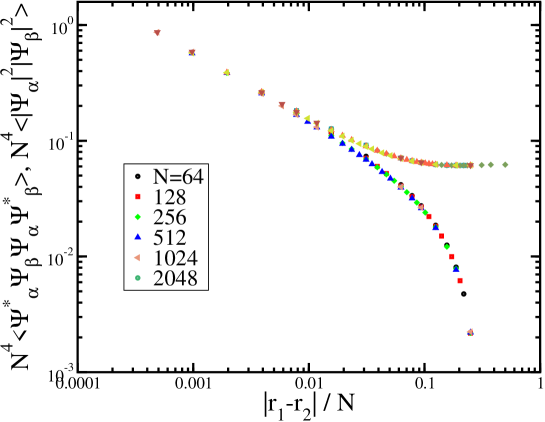
Figure 3: Hartree and Fock contributions to the wave function correlator ${\mathcal{K}}_{1}$ as defined in Eq. (7) for pairs of wavefunctions neighboring in energy. It is seen that in the scaling regime both correlation functions follow the same power law, including the exponent and the amplitude. The corresponding exponent $\Delta_{2}\simeq-0.52$ is known from the multifractal analysis [1].

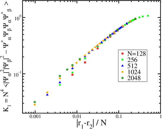
Figure 4: Correlator ${\mathcal{K}}_{1}$ representing the difference of the two functions shown in Fig. 3. The leading power laws cancel and ${\mathcal{K}}_{1}$ is determined by the subleading contributions. Two types of deviations from pure power-law behavior (straight line in the double-log scale) are seen. At small distances the data collapse is not perfect due to corrections to scaling originating from the ultraviolet cutoff scale (lattice constant). At large distances deviations from the power-law scaling are caused by $|{\bf r_{1}}-{\bf r_{2}}|$ approaching $N$. The extracted value of the power-law exponent is $\mu_{2}\simeq 0.62\pm 0.05$.

Figure 4 shows the correlator ${\mathcal{K}}_{1}$ representing the difference of the two functions shown in the previous plot, Fig. 3. As emphasized above, the leading power-law contributions to the Hartree and Fock terms cancel, so that ${\mathcal{K}}_{1}$ is determined by subleading contributions. For a pure power-law scaling behavior we would have a straight line in the double logarithmic scale. We observe two types of deviations from this behavior. At large distances ($|{\bf r}_{1}-{\bf r}_{2}|/N\gtrsim 0.1$) there is a considerable curvature which is related to higher subleading terms. At small distances the data collapse is not perfect due to deviations from scaling related to the ultraviolet cutoff scale (lattice constant) $a$ which leads to emergence of an additional scaling parameter $a/|{\bf r_{1}}-{\bf r_{2}}|$. The numerical analysis yields the power-law exponent $\mu_{2}\simeq 0.62\pm 0.05$.

In Fig. 5 we show the correlation function ${\mathcal{K}}_{2}$ at fixed small distance between pairs of the points, $|{\bf r}_{1}-{\bf r}_{2}|=|{\bf r}_{3}-{\bf r}_{4}|\equiv\rho$, as a function of the distance $R$ between the pairs. When the system size $N$ increases, the data approach a straight line, corresponding to a power-law dependence on $R$ with the exponent $\simeq 1.25$. This exponent is equal to $2\mu_{2}$ within the uncertainty of our numerical analysis. Therefore, within our accuracy the exponent $\alpha$ defined in Eq. (17) is indistinguishable from zero.

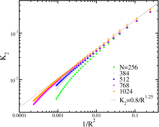
Figure 5: Correlator ${\mathcal{K}}_{2}$ at fixed small distances $|{\bf r}_{1}-{\bf r}_{2}|=|{\bf r}_{3}-{\bf r}_{4}|$ as a function of the distance $R$ between the pairs ${\bf r}_{1,2}$ and ${\bf r}_{3,4}$. Evolution of ${\mathcal{K}}_{2}$ with system size $N$ is shown for a quartett of neighboring energies. The average is over $10^{6}$ samples with two quartetts selected for each sample; the error bars give one standard deviation to indicate the residual statistical uncertainty. It is seen that with increasing $N$ the data approach the straight line, corresponding to a power-law dependence. The corresponding exponent is $\simeq 1.25$, i.e. equal to $2\mu_{2}$ within the numerical uncertainty, implying that $\alpha\simeq 0$.

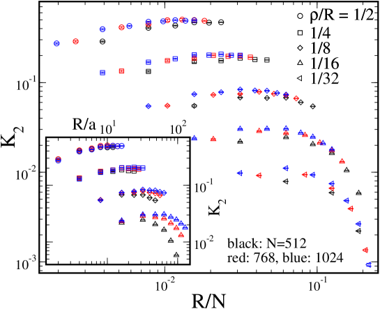
Figure 6: Scaling behavior of ${\mathcal{K}}_{2}$ as a function of $R/N$ for a fixed distance ratio, $\rho/R=1/2,1/4,1/8,1/16,1/32$. Different colors correspond to different system sizes (black: 512, red: 768, blue: 1024). According to Eq. (17), we expect the scaling $\propto(R/N)^{\alpha}$ for $R/N\ll 1$. This scaling behavior is represented by a plateau at intermediate values of $R/N$, yielding $\alpha$ close to zero. At larger $R/N$ we see deviations from a straight line, since other contributions (scaling with higher irrelevant exponents) become significant. At small $R$ deviations from the data collapse are due to corrections in $a/\rho$. Inset: same data replotted as a function of $R/a$. At small distances no $N$-dependence is observed. This confirms that deviations from a simple power-law scaling (straight line) are controlled by $a/\rho$.

The above result on the exponent $\alpha$ is further supported by Fig. 6 where the correlation function ${\mathcal{K}}_{2}$ is plotted as a function of $R/N$ for fixed $\rho/R$. According to Eq. (17), this is a direct way to determine the exponent $\alpha$. We see that at $R/N\lesssim 0.1$ the plots are almost flat, which implies $\alpha\simeq 0$. At small $R$ we observe again the deviations from scaling controlled by the parameter $a/\rho$, as demonstrated in the inset.

To make the scaling properties of ${\mathcal{K}}_{2}$ particularly clear, we replot in the left panel of Fig. 7 the data of Fig. 6, multiplying each trace by $(\rho/R)^{-2\mu_{2}}$ with $2\mu_{2}=1.25$. It is seen that all data (full symbols) collapse on a single-parameter scaling curve showing the dependence of ${\mathcal{K}}_{2}(\rho/R)^{-2\mu_{2}}$ on $R/N$. This confirms that the value of $\mu_{2}$ is correct. The open symbols show the data points for three smallest values of $\rho$; they deviate from the scaling curve due to corrections in $a/\rho$. The plateau of the single-parameter scaling curve at small values of $R/N$ yields $\alpha\simeq-0.05\pm 0.1$ (see the inset in the left panel of Fig. 7 where the same data are shown on a log-log scale). The single-parameter scaling curve is also shown in the right panel of Fig. 7 on the double-linear scale.

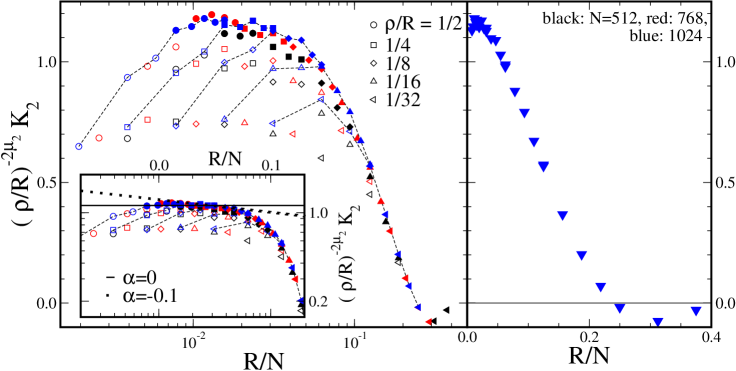
Figure 7: Left panel: Scaling of $(\rho/R)^{-2\mu_{2}}{\mathcal{K}}_{2}$ assuming a critical index $\mu_{2}=0.625$. Different symbols correspond to different values of the ratio $\rho/R$; different colors to different system sizes $N$, as in Fig. 6. Deviations from the single parameter scaling for smallest $\rho$ (open symbols) are due to corrections controlled by $a/\rho$. Inset: Same data on a log-log scale. Solid line (corresponding to $\alpha=0$) and dotted line (corresponding to $\alpha=-0.1$) indicate the power-law scaling region and show the uncertainty range for the numerical value of the exponent $\alpha$. Right panel: Single-parameter scaling function (as obtained from the data points shown by full symbols in the left panel) on the double-linear scale.

To summarize, we have found the values $\mu_{2}\simeq 0.62\pm 0.05$ and $\alpha\simeq-0.05\pm 0.1$ for the critical exponents describing the correlation functions of interest. These values nicely agree with those previously obtained by Lee and Wang [18]. It should be stressed, however, that we used systems of a linear size an order of magnitude larger than in Ref. [18]. The large system sizes $N\gtrsim 500$ were crucially important for our scaling analysis shown in Fig. 7. Indeed, it is seen there that the scaling function reaches the expected power-law behavior $\propto(R/N)^{\alpha}$ (with $\alpha$ close to zero) only at relatively small values of the scaling argument, $R/N\lesssim 0.05$. On the other hand, the scale $\rho$ cannot be too small, since the corrections controlled by the parameter $a/\rho$ become substantial unless $\rho/a\gtrsim 4$. Finally, we have a condition $R\gg\rho$, which in practice requires that $R/\rho\gtrsim 2$. Combining all this, we see that in order to have a window of good power-law scaling, we need $N$ considerably larger than $2\times 4\times 20=160$. Our system sizes reasonably satisfy this requirement. As a result, we get a window of $R/N$ approximately between 0.007 and 0.05, where the required scaling takes place. On the other hand, relatively small system sizes did not allow the authors of Ref. [18] to obtain this scaling window. Indeed, their Fig. 2 shows a function that changes by several orders of magnitude without any developed saturation plateau. While the authors of Ref. [18] argued correctly in favor of small $\alpha$, it seems difficult to make a reliable conclusion concerning $\alpha$ with only data for small systems (as shown in their Fig. 2) at hand.

Using the obtained values of $\mu_{2}$ and $\alpha$, we can calculate the exponents controlling the interaction effects, see Eqs. (59) and (60). Assuming the case of “most short-range interaction”, $\lambda>2+\mu_{2}\simeq 2.62$, we get

$$p\simeq 1.62\ ;\qquad z_{T}\simeq 1.23\ ;\qquad\kappa\simeq 0.346\,.$$ (63)

While calculating $\kappa$ in Eq. (63), we used the value of the localization length exponent, $\nu\simeq 2.35$ found by Huckestein and coauthors (see the review [33]) and confirmed by several later works. Recently, Slevin and Ohtsuki [34] reconsidered the problem and concluded that corrections to scaling are much larger that was previously thought. As a result, they obtained a larger value of the localization length critical exponent, $\nu\simeq 2.59$. If this value as used, we get a somewhat smaller result for the exponent $\kappa$,

$$\kappa\simeq 0.314\,.$$ (64)

We will compare these values to existing experimental results in Sec. 5, where we will also discuss expected modifications in the case of Coulomb interaction.

4.3 Anderson transition in $d=3$ and higher dimensions

For the Anderson transition in $d=3$ the $\epsilon$-expansion cannot give quantitatively reliable predictions for critical exponents. Therefore, one has to rely on numerical simulations. The critical exponent of the localization length for the unitary symmetry class was found to be $\nu=1.43\pm 0.04$ [35]. While the most relevant multifractal exponents (characterizing the scaling of moments of wave function amplitudes) $\Delta_{q}$ have been extensively studied, no numerical analysis of the subleading exponents, in partiuclar $\mu_{2}$ and $\alpha$, has been done to the best of our knowledge. This is an interesting direction for future research. In particular, an intriguing question is whether the condition $d-2\mu_{2}+\alpha>0$ becomes violated in 3D (or, more generally at sufficiently high dimensionality). According to Eq. (19), this would result in a change of the behavior of the dephasing rate $1/\tau_{\phi}$ that would become dependent on the exponent $\alpha$.

4.4 Discussion: Consistency of the calculation of the dephasing rate and the transition width

Having completed the calculation of the dephasing rate and of the localization transition width, we have to come back to the assumptions made in course of the calculation and check their consistency. Specifically, we have made two important assumptions: on the averaging procedure and on the critical character of the wave functions involved.

4.4.1 Critical character of wave functions

When we calculated the dephasing rate as the imaginary part of the self energy ${\rm Im}\>\Sigma(E,\varepsilon)$, we assumed that the zero energy (i.e. the position of the chemical potential $\mu$) is exactly at the critical point. On the other hand, the obtained transition width scales as $\propto T^{\kappa}$ with $\kappa<1$, i.e. it is much larger than $T$. Therefore, it is important to check that finite deviation of $\mu$ from criticality, $|\mu-\mu_{c}|\propto T^{\kappa}$ does not invalidate the calculation. This detuning from criticality will produce a characteristic scale (localization or correlation length), $\xi_{\mu}\propto|\mu-\mu_{c}|^{-\nu}$ that determines the range of critical behavior of correlation functions. Inserting here $|\mu-\mu_{c}|\propto T^{\kappa}$, we get $\xi_{\mu}\propto T^{-1/z_{T}}$, which is just the condition $\xi_{\mu}=L_{\phi}$ that we used to determine the transition width. Therefore, for characteristic detuning from critical energy $\sim|\mu-\mu_{c}|$ the critical correlations extend up to $L_{\phi}\propto T^{-1/z_{T}}$. On the other hand, the range of spatial integration in Eq. (18) was set by the thermal length $L_{T}\propto T^{-1/d}$. We thus have to compare $L_{\phi}$ and $L_{T}$. Since $z_{T}<d$, we have $L_{\phi}\gg L_{T}$, which justifies the calculation.

4.4.2 Averaging of dephasing rate

While evaluating $\tau_{\phi}$, we have performed averaging over the disorder realizations. A natural question to ask is whether this is a valid procedure. Indeed, we know that in the localized phase such an averaging breaks down with lowering temperature [36] since the level spacing of those states with which the given state is coupled becomes larger than the averaged dephasing rate. As a consequence the Golden-rule calculation of the dephasing rate that treats these states essentially as a continuum breaks down. However, in the critical regime we are considering the situation is essentially different. As we discussed in Sec. 4.4.1, the localization length $\xi_{\mu}$, which is equal to the dephasing $L_{\phi}$, increases (with lowering temperature) faster than $T^{-1/d}$. As a result, the number of states contributing to the dephasing rate of a given state—i.e. of states located in the energy interval of width $T$ and in the spatial volume (area for $d=2$) of extension $\xi_{\mu}=L_{\phi}\propto T^{-1/z_{T}}$ increases as a power law with decreasing $T$. In this situation, the dephasing rate $\tau_{\phi}$ is a self-averaging quantity.

4.4.3 Other possible contributions to dephasing

Strictly speaking, what we have calculated in this paper is the lowest-order (golden rule) dephasing rate governed by the generic range of frequencies ($\Omega\sim\varepsilon^{\prime}\sim T$). Thus, putting it rigoristically, we have calculated the upper bound on $L_{\phi}$, and, consequently, the lower bound on $z_{T}$ and upper bound on $\kappa$. Indeed, formally one cannot exclude the possibility that a contribution of a different scaling domain of frequency and spatial variables to the lowest-order dephasing rate or contribution of higher order in $U$ is larger. Our preliminary analysis indicate that this does not happen (apart from possible logarithmic corrections to scaling) for critical points with relatively small anomalous exponents, like Anderson transition in $2+\epsilon$ dimensions and quantum Hall transition which are in the focus of this paper. It is a challenging task to understand whether such exotic contributions may dominate the dephasing rate at transitions with strong fluctuations, like Anderson transition in higher dimensionalities. The complexity of the problem is related to the fact that the other contributions are controlled by wave function correlations characterized by different scaling exponents. We postpone this analysis to future work.

5 Coulomb interaction and experiment

Most of this paper is devoted to the case of short-range interaction, when the interaction irrelevant in the RG sense and the dephasing rate is controlled by critical properties at the non-interacting fixed point. In this section we briefly discuss the present understanding of the case of long-range Coulomb interaction and summarize the available experimental results.

5.1 Criticality at Anderson and quantum Hall transitions with Coulomb interaction

For long-range ($1/r$) Coulomb interaction, the dephasing rate is proportional to temperature, $1/\tau_{\phi}\sim T$. It is easy to see how the short-range interaction results develop into this behavior with decreasing $\lambda$. Indeed, the lowest possible “short-range” $\lambda$ is $\lambda=d$, for which the first line of Eq. (21) should be used, yielding $1/\tau_{\phi}\sim T$. Further decreasing $\lambda$ does not change the scaling of the dephasing rate anymore, since $1/\tau_{\phi}$ cannot vanish slower than temperature in a system with meaningfully defined fermionic excitations. The result $1/\tau_{\phi}\sim T$ implies that the scaling with temperature is the same as with frequency, which is usually the case at “standard” quantum phase transitions. Therefore, in contrast to the case of short-range interaction, for the long-range interaction there is no need in distinguishing the dynamical exponents governing the frequency and temperature scaling, $z_{T}=z$.

On the other hand, the long-range interaction problem is characterized by several dynamical exponents controlling the frequency scaling of different observables [3, 4]. The reason for this complex behavior is the existence of several conserved quantities. Let us assume for simplicity that the system is spin-polarized (or else, the spin invariance is completely broken, e.g., by spin-orbit interaction or by magnetic impurities). Then the conserved quantities are particle number and energy. As a consequence, there are two Goldstone modes, which are characterized by poles of the diffusion type but with a non-trivial scaling, $q^{z_{i}}\sim\omega$. In notations of Ref. [4] $z_{1}$ corresponds to the energy mode, and $z_{3}$ to the density mode.

The exponent $z_{1}$, which was denoted as $\zeta$ by Finkelstein [3] and as $2+\gamma^{*}$ in Ref. [39], governs the renormalization of frequency in the $\sigma$-model action. It is this exponent that plays a role of $z_{T}=z$ for the problem we are considering, i.e., it controls the scaling of the dephasing length $L_{\phi}\sim\tau_{\phi}^{1/z}$ and therefore enters the formula

$$\kappa=1/\nu z\ ;\qquad\qquad z\equiv z_{1}$$ (65)

for the exponent $\kappa$ of the transition width.

We emphasize the distinction between different dynamical exponents, since this was not always appreciated by researchers in the field and has led to confusions and controversies. A number of authors used the exponent $z_{3}$, which is equal to 1 for the case of $1/r$ interaction, instead of $z_{1}$ in Eq. (65). This is incorrect. To make this point clear, it is constructive to draw an analogy with a 2D problem: the critical problem in $2+\epsilon$ dimensions with small $\epsilon$ bears a lot of similarities with a 2D problem with large conductance. The exponent $z_{3}=1$ exists also in 2D: it controls the plasmon pole in the (reducible) density response function. It is well known, however, that the plasmon pole does not affect the conductivity; in particular, the dephasing rate is recalculated in dephasing length according to a diffusion formula $L_{\phi}\propto(D\tau_{\phi})^{1/2}$, corresponding to $z=2$. Furthermore, the localization effects are controlled by cooperons and by “delayed diffusons” [37, 38] that are given by ladder diagramms without interaction vertex corrections. These are just modes that acquire the $z_{1}$ dynamical scaling at criticality.

In $2+\epsilon$ dimensions for the considered symmetry class (time reversal and spin symmetries are broken; denoted as “MI(LR)” in Ref. [4] ), the $\beta$-function, the critical point, and the exponents $\nu$ and $z$ are known up to the two-loop order [39]:

$$\beta(t) = \epsilon t-2t^{2}-4At^{3}\ ;\qquad\qquad A\simeq 1.64\ ;$$ (66)

$$t_{*} = \frac{\epsilon}{2}-\frac{A}{2}\epsilon^{2}+O(\epsilon^{3})$$ (67)

$$\nu = \frac{1}{\epsilon}-A+O(\epsilon)\ ;$$ (68)

$$z = 2+\frac{\epsilon}{2}+\left(\frac{A}{2}-\frac{\pi^{2}}{24}-\frac{3}{4}\right)\epsilon^{2}+O(\epsilon^{3})\,.$$ (69)

Substituting (68) and (69) into (65), we get

$$\kappa=\frac{\epsilon}{2}+\left(\frac{A}{2}-\frac{1}{8}\right)\epsilon^{2}+O(\epsilon^{3})\,.$$ (70)

For the quantum Hall transition with Coulomb interaction not much can be said concerning the values of the exponents on the theoretical level. Since the transition happens in the strong-coupling regime of the $\sigma$-model, no reliable analytical predictions can be made. The numerical analysis is also very difficult: (i) exact diagonalization can be performed for small systems only, which is not suffucient for determining the critical behavior, and (ii) no approximate method that would allow to get the interacting critical exponents has been developed. On general grounds, and using the analogy with the Anderson transition in $2+\epsilon$ dimensions, one can say that there is no reasons to expect that the exponents $\nu$ and $z$ (as well as any other exponents) would take the same values as for the non-interacting system. Also, there is no reasons for the exponent $z\equiv z_{1}$ to take any “simple” value (like, e.g., 1 or 2).

5.2 Experiments on localization transition in interacting systems

5.2.1 Anderson transition in 3D

The 3D localization transition was extensively studied on doped semiconductor systems, such as Si:P, Si:B, Si:As, Ge:Sb. In most of the works, samples with a substantial degree of compensation [i.e. acceptors in addition to donors, e.g. Si:(P,B)] were used, which allows one to vary the amount of disorder and the electron concentration independently. On these samples, values of the conductivity exponent $s$ in the vicinity of $s\approx 1$ were reported [40] with scattering of values and the uncertainties of the order of $10\%$. A similar result was obtained for an amorphous material Nb_xSi_1-x. We recall that $s$ is expected to be equal in 3D to the localization length exponent $\nu$ according to the scaling relation $s=\nu(d-2)$.

On the other hand, the early study of the transition in undoped Si:P [41] gave an essentially different result, $s\approx 0.5$, which is also in conflict with the Harris inequality $\nu>2/d$. This discrepancy was resolved in [42] where it was found that the actual critical region in an uncompensated Si:P is rather narrow and that the scaling analysis restricted to this range yields $s\approx 1.3$. A more recent study along these lines [16] yielded $s=1.0\pm 0.1$, in agreement with the values obtained for samples with compensation. It thus appears that for the orthogonal symmetry class (preserved time-reversal and spin invariances) the experiments have converged to the value $s=1.0\pm 0.1$. (The only exception is a recent experiment on uncompensated Si:B [17] where a larger value was found, $s\approx 1.6$. A possible explanation is that the temperatures reached in this work were not sufficiently low. Another possibility is that Si:B belongs to a different universality class, in view of stronger spin-orbit scattering.) Results on the dynamical scaling are much scarcer: it was found to be $z=2.94\pm 0.3$ in Ref. [16] and $z\approx 2$ in Ref. [17].

The fact that the experimental value $s\approx 1$ differs from the result $s=\nu\simeq 1.57\pm 0.02$ [43] for non-interacting systems of the orthogonal symmetry class is in line with the general expectation that the Coulomb interaction affects the critical exponents.

5.2.2 Quantum Hall transition

Experiments on the integer quantum Hall plateau transition determine the width of the critical region (peak in $\sigma_{xx}$ and plateau transition in $\sigma_{xy}$), which scales with the temperature $T$ as $\Delta B{\propto}T^{\kappa}$. The early measurements of the exponent $\kappa$ performed on InGaAs/InP samples yielded $\kappa{=}0.42{\pm}0.04$ [14]. A number of works discussed the effect of macroscopic inhomogeneities [46, 47, 15] that complicate observation of the true IQH critical behavior. The final conclusion is [15] that for short-range disorder, when the true IQH criticality can be achieved, $\kappa{=}0.42{\pm}0.01$, in agreement with the result of Ref. [14]. A very recent work [48] where the quantum Hall transition in AlGaAs/AlGaAs samples was analyzed down to very low temperatures ($1\>{\rm mK}$) confirmed this result for $\kappa$.

Experimental determination of the exponents $\nu$ and $z_{T}$ is a highly complicated problem. The values reported in the literature are $\nu\simeq 2.3$ [44, 45] and $z_{T}\simeq 1$ [48], with the scattering of data of the order of $10\%$. Our feeling, however, is that these data might be essentially affected by systematic errors. Specifically, the works [44, 45] where $\nu$ was measured reported the values of $\kappa$ in the range from 0.6 to 0.8 (i.e. much larger than the true exponent 0.42). It is understood now that such increased values of $\kappa$ correspond to situations where macroscopic inhomogeneities do not allow one to observe the true quantum Hall criticality. In such a situation the observed $\nu$ may also differ from the actual quantum Hall value. Further, the most direct determination of $z$ [48] was based on the analysis of the data for different system sizes, which is a nice way to find the dephasing length. However, there may be a problem [49] related to the fact that disorder strength was apparently correlated with the sample width (see Fig.3a of Ref. [48]). As a result, the natural temperature scale (mean free time) for different samples is different. This is not a small effect: as is seen from Fig.3a of Ref. [48] changing the sample width by factor of 5 not only changes the saturation temperature by factor of $\approx 5$ but simultaneously changes the characteristic temperature scale by factor of $\approx 2.5$. In our view, this might considerably affect the determination of the dynamical exponent $z_{T}$. It seems that more experimental work may be needed to overcome these difficulties related to systematic errors in evaluation of $z_{T}$ and $\nu$.

Summarizing the experimental findings, the most updated values of the exponents are $\nu=2.3{\pm}0.1$, $\kappa{=}0.42{\pm}0.01$, and $z_{T}\equiv z\simeq 1.0\pm 0.1$, although the error in determination of $\nu$ and $z_{T}$ may be considerably underestimated due to systematic errors. Let us remind the reader that the theoretical results for the case of short-range interaction are as follows: the value of $\nu$ ranges from 2.35 to 2.59, $z_{T}\simeq 1.23$, and $\kappa=1/\nu z_{T}$ is in the range from 0.314 to 0.346. It appears that the difference in values of the exponents between the cases of short-range (theory) and long-range (experiment) interactions is not so large: $\lesssim 10\%$ for $\nu$, $\lesssim 20\%$ for $z_{T}$, and $\lesssim 30\%$ for $\kappa$. (Again, for $\nu$ and $z_{T}$ might be large due to systematic errors.) Nevertheless, the difference demonstrates that the current experiments on criticality at quantum Hall transitions cannot be explained in terms of the non-interacting fixed point. An experimental realization of the short-range interaction universality class remains a challenging issue for future research.

6 Conclusions

To summarize, we have studied the scaling properties of dephasing rate at critical point of the localization transition. We have considered the case of a short-range interaction in systems with no spin degeneracy (or broken spin-rotation symmetry). In this situation the interaction is found to be RG-irrelevant, and the critical properties can be studied by performing the scaling analysis near the non-interacting fixing point.

More specifically, we considered problems with broken time-reversal invariance: the quantum Hall transition and the Anderson transition in $2+\epsilon$ dimensions. Our work combined analytical and numerical analysis. In the analytical part, we used the framework of the non-linear $\sigma$ model. We identified operators controlling the scaling of the correlation function that determines the dephasing rate. Further, we performed their RG analysis in $2+\epsilon$ dimensions. This allowed us to find the analytical results for the exponents $p$, $z_{T}$, and $\kappa$ governing the temperature scaling of the dephasing rate, dephasing length, and the transition width.

The numerical analysis was used to obtain critical exponent at the quantum Hall transition. Our results for the exponents largely agree with those obtained in Refs. [18, 19]. However, our system sizes are much largely than those studied in Ref. [18] that was crucial for getting a window of distances where corrections to power-law scaling are small.

Experimental results on localization transition with short-range interaction are extremely desirable. In the case of quantum Hall transition one could imagine screening of the Coulomb interaction by an external gate. It would be extremely interesting to observe the change of the exponents compared to the case of long-range interaction. This is a challenging task, especially since the difference between the exponents appears to be not so large (see Sec. 5.2.2). For 3D Anderson transition, its experimental realization and investigation in cold-atoms systems would be of great importance.

On the theoretical side, the wave function correlation exponents $\mu_{2}$ and $\alpha$ need to be evaluated for 3D Anderson transition (with and without time-reversal invariance), in order to predict the behavior of the dephasing rate and thus the exponents $p$, $z_{T}$, and $\kappa$. More generally, investigation of the statistics of wave functions at criticality beyond the leading multifractal behavior represents an important research field. It would be interesting to understand the evolution of this statistics (which includes the statistics of Hartree-Fock matrix elements) from the regime of weak to strong multifractality, as it has been done for the spectrum of leading multifractal exponents $\Delta_{q}$ [1].

7 Acknowledgements

The work was supported by RFBR Grant Nos. 09-02-12206 and 09-02-00247, the Council for grants of the Russian President Grant No. MK-125.2009.2, RAS Programs “Quantum Physics of Condensed Matter”, “Fundamentals of nanotechnology and nanomaterials”, the Russian Ministry of Education and Science under contract No. P926, by the Center for Functional Nanostructures of the Deutsche Forschungsgemeinschaft, by the SPP “Graphene” of the DFG, and by the EUROHORCS/ESF EURYI Awards scheme. S.B. and F.E. thank I. Kondov for support in optimizing the computer code used for the numerical simulations. I.S.B. is grateful to A. Pruisken for useful discussions. I.S.B. is grateful to the Institute of Condensed Matter Theory and Institute of Nanotechnology of Karlsruhe Institute of Technology for hospitality.

Appendix A Correlation function $\mathcal{K}_{1}$.

In this Appendix we demonstrate that the function $\mathcal{K}_{1}$ corresponds to the eigenoperator $P_{1,1}$. The function $\mathcal{K}_{1}$ can be expressed in terms of the exact single-particle Green’s functions $G_{R,A}(\bm{r},\bm{r}^{\prime})$:

$$\mathcal{K}_{1}=\frac{\Delta^{2}}{\pi^{2}}\Biggl{\langle}\operatorname{Im}G_{E+\omega}^{R}(\bm{r}_{1},\bm{r}_{1})\operatorname{Im}G_{E}^{R}(\bm{r}_{2},\bm{r}_{2})-\operatorname{Im}G_{E+\omega}^{R}(\bm{r}_{2},\bm{r}_{1})\operatorname{Im}G_{E}^{R}(\bm{r}_{1},\bm{r}_{2})\Biggr{\rangle}.$$ (71)

Following standard steps (see e.g. Ref. [25]), we obtain

$$\mathcal{K}_{1}=\frac{\Delta^{2}}{(2\pi\gamma)^{2}}\left\langle\operatorname{tr}\Lambda Q_{aa}(\bm{r}_{1})\operatorname{tr}\Lambda Q_{bb}(\bm{r}_{2})+\operatorname{tr}\Lambda Q_{ab}(\bm{r}_{1})\Lambda Q_{ba}(\bm{r}_{2})\right\rangle\,,$$ (72)

where repica indices $a,b$ are different, $a\neq b$, which reflects the fact that we are dealing with two different eigenstates. Since we are interested in the case for which two points are close to each other (say, $|\bm{r}_{1}-\bm{r}_{2}|$ is of order of a few lattice constants $a$), we can consider the arguments of $Q$ matrices as equal. Below the arguments are omitted.

Let us define two operators bilinear in $Q$:

$$\tilde{O}_{\pm}[Q]=\operatorname{tr}\Lambda Q_{ab}\Lambda Q_{ba}\pm\operatorname{tr}\Lambda Q_{ab}\operatorname{tr}\Lambda Q_{ba}.$$ (73)

Clearly, $\mathcal{K}_{1}\propto\tilde{O}_{+}$. In order to obtain the $U(n)\times U(n)$ invariant expression let us perform the following global rotation in the $Q$-matrix space,

$$Q(\bm{r})\to U^{-1}Q(\bm{r})U,\qquad U^{pp^{\prime}}_{ab}=U^{p}_{ab}\delta^{pp^{\prime}},$$ (74)

which does not change the action $S_{\sigma}$. Thus, we introduce the averaged, operators

$$O_{\pm}[Q]=\left\langle\operatorname{tr}\Lambda[U^{-1}QU]_{ab}\Lambda[U^{-1}QU]_{ba}\pm\operatorname{tr}\Lambda[U^{-1}QU]_{ab}\operatorname{tr}\Lambda[U^{-1}QU]_{ba}\right\rangle_{U}$$ (75)

where $\langle\dots\rangle_{U}$ denotes averaging over $U(n)\times U(n)$ global rotations. Since the action $S_{\sigma}$ is invariant under $U(n)\times U(n)$, the $\sigma$-model averages of $O_{\pm}[Q]$ and $\tilde{O}_{\pm}[Q]$ are equal,

$$\langle\tilde{O}_{\pm}[Q]\rangle=\langle O_{\pm}[Q]\rangle,$$ (76)

In order to perform the averaging over $U(n)\times U(n)$ rotations, we use the following results [50]:

$$\langle(U^{-1})^{p}_{a\alpha}U^{p}_{\beta b}\rangle_{U}=V_{1}\delta_{ab}\delta_{\alpha\beta},$$ (77)

$$\langle(U^{-1})^{p}_{a\alpha}U^{p}_{\beta b}(U^{-1})^{p}_{c\gamma}U^{p}_{\mu d}\rangle_{U}=V_{1,1}\left[\delta_{ab}\delta_{\alpha\beta}\delta_{cd}\delta_{\gamma\mu}+\delta_{ad}\delta_{\alpha\mu}\delta_{bc}\delta_{\beta\gamma}\right]$$

$$+V_{2}\left[\delta_{bc}\delta_{\alpha\beta}\delta_{da}\delta_{\gamma\mu}+\delta_{ab}\delta_{\alpha\mu}\delta_{cd}\delta_{\beta\gamma}\right]\,,$$ (78)

where $V_{1}$, $V_{1,1}$ and $V_{2}$ are given in Table 2. The index $p=\pm$ distinguishes between the retarded and advanced sectors, i.e. $(U^{+},U^{-})$ is an element of $U(n)\times U(n)$. The averaging over $U^{+}$ and $U^{-}$ is carried out independently.

Performing the averaging, we obtain the following $U(n)\times U(n)$ invariant results:

$$O_{\pm}[Q]=\frac{2n\pm 1}{2n^{2}(n\pm 1)}\left\{\operatorname{Tr}(\Lambda Q)^{2}\pm(\operatorname{Tr}\Lambda Q)^{2}\right\}\pm\frac{(2n-1)\mp 2n}{2n^{2}(n\pm 1)}\operatorname{Tr}\mathbf{1}.$$ (79)

It is not difficult to check that operators $O_{\pm}$ are eigenoperators under the action of the renormalization group: $O_{-}=P_{2}$ and $O_{+}=P_{1,1}$ .

$V_{1}=\frac{1}{n}$,

$V_{1,1}=\frac{n}{n(n^{2}-1)}$,   $V_{2}=-\frac{1}{n(n^{2}-1)}$,

$V_{1,1,1}=\frac{n^{2}-2}{n(n^{2}-1)(n^{2}-4)}$,  $V_{2,1}=-\frac{n}{n(n^{2}-1)(n^{2}-4)}$,   $V_{3}=\frac{2}{n(n^{2}-1)(n^{2}-4)}$,

$V_{1,1,1,1}=\frac{6-8n^{2}+n^{4}}{n^{2}(n^{2}-1)(n^{2}-4)(n^{2}-9)}$,   $V_{2,1,1}=\frac{n(4-n^{2})}{n^{2}(n^{2}-1)(n^{2}-4)(n^{2}-9)}$,  $V_{2,2}=\frac{6+n^{2}}{n^{2}(n^{2}-1)(n^{2}-4)(n^{2}-9)}$,

$V_{3,1}=\frac{2n^{2}-3}{n^{2}(n^{2}-1)(n^{2}-4)(n^{2}-9)}$,   $V_{4}=-\frac{5n}{n^{2}(n^{2}-1)(n^{2}-4)(n^{2}-9)}$

Table 2: Coefficients $V_{j}$ for averaging over the unitary group $U(n)$.

Appendix B Correlation function $\mathcal{K}_{2}$.

In this Appendix, we express the correlation function $\mathcal{K}_{2}$ in terms of basis operators $O_{j}[Q]$. This requires, in addition to bilinear operators considered in Appendix A, introducing operators of the fourth order in $Q$. As in the previous Appendix, it is convenient to perform global transformation (74) and average over $U(n)\times U(n)$ rotations. Then $\mathcal{K}_{2}$ becomes

$$\mathcal{K}_{2}=\frac{\Delta^{4}}{(2\pi\gamma)^{4}}\Bigl{\langle}R_{1}[Q]+R_{2}[Q]\Bigr{\rangle}$$ (80)

where

$$R_{1}[Q]=\langle\operatorname{tr}\Lambda(U^{-1}QU)_{ab}\Lambda(U^{-1}QU)_{ba}\operatorname{tr}\Lambda(U^{-1}QU)_{cd}\Lambda(U^{-1}QU)_{dc}\rangle_{U},$$ (81)

$$R_{2}[Q]=\langle\operatorname{tr}\Lambda(U^{-1}QU)_{ab}\Lambda(U^{-1}QU)_{bc}\Lambda(U^{-1}QU)_{cd}\Lambda(U^{-1}QU)_{da}\rangle_{U}..$$ (82)

In order to perform averaging over $U(n)\times U(n)$ rotations it is convenient to use diagrammatic technique developed in Ref. [51]. The result is as follows

$$R_{1}[Q] = \sum_{p=\pm}\Bigl{\{}V_{2,2}(\operatorname{Tr}Q_{p})^{4}+(4V_{4}+2V_{2,1,1})\operatorname{Tr}Q_{p}^{2}(\operatorname{Tr}Q_{p})^{2}$$ (83)

$$+8V_{3,1}\operatorname{Tr}Q_{p}^{3}\operatorname{Tr}Q_{p}+(2V_{2,2}+V_{1,1,1,1})\operatorname{Tr}Q_{p}^{2}\operatorname{Tr}Q_{p}^{2}$$

$$+(4V_{2,1,1}+2V_{4})\operatorname{Tr}Q_{p}^{4}-4V_{1}V_{2,1}(\operatorname{Tr}Q_{p})^{2}\operatorname{Tr}A_{p}$$

$$-4V_{1}V_{1,1,1}\operatorname{Tr}Q_{p}^{2}\operatorname{Tr}A_{p}-8V_{1}V_{2,1}\operatorname{Tr}(A_{p}Q_{p}^{2})$$

$$-8V_{1}V_{3}\operatorname{Tr}Q_{p}\operatorname{Tr}A_{p}Q_{p}+2(V^{2}_{1,1}+V^{2}_{2})(\operatorname{Tr}A_{p})^{2}$$

$$+4V_{1,1}V_{2}\operatorname{Tr}A_{p}^{2}+V_{1,1}^{2}\operatorname{Tr}Q_{p}^{2}\operatorname{Tr}Q^{2}_{-p}$$

$$+2V_{2}V_{1,1}\operatorname{Tr}Q^{2}_{p}(\operatorname{Tr}Q_{-p})^{2}+V_{2}^{2}(\operatorname{Tr}Q_{p})^{2}(\operatorname{Tr}Q_{-p})^{2}\Bigr{\}},$$

and

$$R_{2}[Q] = \sum_{p=\pm}\Bigl{\{}V_{4}(\operatorname{Tr}Q_{p})^{4}+(4V_{3,1}+2V_{2,2})\operatorname{Tr}Q_{p}^{2}(\operatorname{Tr}Q_{p})^{2}$$ (84)

$$+4(V_{4}+V_{2,1,1})\operatorname{Tr}Q_{p}^{3}\operatorname{Tr}Q_{p}+(V_{4}+2V_{2,1,1})\operatorname{Tr}Q_{p}^{2}\operatorname{Tr}Q_{p}^{2}$$

$$+(V_{2,2}+V_{1,1,1,1}+4V_{3,1})\operatorname{Tr}Q_{p}^{4}-4V_{1}V_{3}(\operatorname{Tr}Q_{p})^{2}\operatorname{Tr}A_{p}$$

$$-4V_{1}V_{2,1}\operatorname{Tr}Q_{p}^{2}\operatorname{Tr}A_{p}-4V_{1}(V_{3}+V_{1,1,1})\operatorname{Tr}(A_{p}Q_{p}^{2})$$

$$-8V_{1}V_{2,1}\operatorname{Tr}Q_{p}\operatorname{Tr}A_{p}Q_{p}+2V_{2}^{2}\operatorname{Tr}Q_{p}\operatorname{Tr}Q_{-p}\operatorname{Tr}A_{p}$$

$$+4V_{2}V_{1,1}\operatorname{Tr}Q_{p}\operatorname{Tr}B_{p}+2V_{1,1}^{2}\operatorname{Tr}B_{p}Q_{p}+2V_{1,1}V_{2}(\operatorname{Tr}A_{p})^{2}$$

$$+(V_{1,1}^{2}+V_{2}^{2})\operatorname{Tr}A_{p}^{2}\Bigr{\}}\,,$$

where the coefficents $V_{j_{1},\ldots,j_{m}}$ are introduced in analogy with Eqs. (77), (78). Specifically, $V_{j_{1},\ldots,j_{m}}$ arises when one averages a product of $j=j_{1}+\ldots+j_{m}$ matrix elements of $U$ and $j$ matrix elements of $U^{-1}$ as a coefficients in front of terms corresponding to $m$ “cycles” of the sizes $j_{1},\ldots j_{m}$. Further, we have introduced the notations

$$Q_{p} = \frac{1+p\Lambda}{2}Q\frac{1+p\Lambda}{2},$$ (85)

$$A_{p} = \frac{1+p\Lambda}{2}Q\frac{1-p\Lambda}{2}Q\frac{1+p\Lambda}{2},$$ (86)

$$B_{p} = \frac{1+p\Lambda}{2}Q\frac{1-p\Lambda}{2}Q\frac{1-p\Lambda}{2}Q\frac{1+p\Lambda}{2}.$$ (87)

Using the expressions for the coefficents $V_{j}$ from Table 2, we can express the operators $R_{1}$ and $R_{2}$ via operators (29)-(35). The result is given in Eq. (28).

References

- [1] F. Evers and A.D. Mirlin, Rev. Mod. Phys. 80, 1355 (2008); A. D. Mirlin, F. Evers, I. V. Gornyi and P. M. Ostrovsky, in 50 years of Anderson localization, ed. by E. Abrahams (World Scientific, 2010), p. 107; Int. J. Mod. Phys. B 24, 1577 (2010).
- [2] B.L. Altshuler and A.G. Aronov, in Electron-Electron Interactions in Disordered Systems, edited by A.L. Efros and M. Pollak (Elsevier, 1985), p.1.
- [3] A.M. Finkelstein, Sov. Sci. Rev. Sect. A 14, 1 (1990); in 50 years of Anderson localization, ed. by E. Abrahams (World Scientific, 2010), p. 385; Int. J. Mod. Phys. B 24, 1855 (2010).
- [4] D. Belitz and T.R. Kirkpatrick, Rev. Mod. Phys. 66, 261 (1994).
- [5] A.M.M.Pruisken, in 50 years of Anderson localization, ed. by E. Abrahams (World Scientific, 2010), p. 503; Int. J. Mod. Phys. B 24, 1895 (2010).
- [6] E. Abrahams, S.V. Kravchenko, and M.P. Sarachik, Rev. Mod. Phys. 73, 251 (2001); S.V. Kravchenko and M.P. Sarachik, Rep. Progr. Phys. 67, 1 (2004); S.V. Kravchenko and M.P. Sarachik, in 50 years of Anderson localization, ed. by E. Abrahams (World Scientific, 2010), p. 361; Int. J. Mod. Phys. B 24, 1640 (2010).
- [7] V.M. Pudalov, M.E. Gershenson, and H. Kojima, in Fundamental Problems of Mesoscopic Physics. Interaction and Decoherence, ed. by I.V. Lerner, B.L. Altshuler, and Y. Gefen, NATO Sci. Series, Kluwer (2004), p. 309.
- [8] S.V. Kravchenko, G.V. Kravchenko, J.E. Furneaux, V.M. Pudalov, and M. D’Iorio, Phys. Rev. B 50, 8039 (1994); S.V. Kravchenko, W.E. Mason, G.E. Bowker, J.E. Furneaux, V.M. Pudalov, and M. D’Iorio, Phys. Rev. B 51, 7038 (1995).
- [9] A. Punnoose and A.M. Finkelstein, Science 310, 289 (2005).
- [10] S. Anissimova, S.V. Kravchenko, A. Punnoose, A.M. Finkel’stein, and T.M. Klapwijk, Nature Phys. 3, 707 (2007).
- [11] D.A. Knyazev, O.E. Omel’yanovskii, V.M. Pudalov, and I.S. Burmistrov, Phys. Rev. Lett. 100, 046405 (2008).
- [12] P. M. Ostrovsky, I. V. Gornyi, and A. D. Mirlin, Phys. Rev. Lett. 105, 036803 (2010).
- [13] M.V. Feigel’man, L.B. Ioffe, V.E. Kravtsov, and E. Cuevas, Annals of Physics 325, 1368 (2010).
- [14] H.P. Wei, D.C. Tsui, M.A. Paalanen, and A.M.M. Pruisken, Phys. Rev. Lett. 61, 1294 (1988).
- [15] W. Li, G. A. Csathy, D. C. Tsui, L. N. Pfeiffer, and K. W. West, Phys. Rev. Lett. 94, 206807 (2005).
- [16] S. Waffenschmidt, C. Pfleiderer, and H. v. Löhneysen, Phys. Rev. Lett. 83, 3005 (1999).
- [17] S. Bogdanovich, M.P. Sarachik, and R.N. Bhatt, Phys. Rev. Lett. 82, 137 (1999).
- [18] D-H. Lee and Z. Wang, Phys. Rev. Lett. 76, 4014 (1996).
- [19] Z. Wang, M.P.A. Fisher, S.M. Girvin, and J.T. Chalker, Phys. Rev. B 61, 8326 (2000).
- [20] M.A. Baranov and A.M.M.Pruisken, Europhys. Lett. 31, 543 (1995).
- [21] E. Abrahams, P.W. Anderson, P.A. Lee, T.V. Ramakrishnan, Phys. Rev. B 24, 6783 (1981).
- [22] F. Wegner, Z. Phys. B 35, 207 (1979).
- [23] H. Levine, S. Libby, and A.M.M. Pruisken, Phys. Rev. Lett. 51 1915 (1983); A.M.M. Pruisken, Nucl. Phys. B 235, 277 (1984).
- [24] A.M.M. Pruisken and I.S. Burmistrov, Ann. Phys. (N.Y.) 316, 285 (2005).
- [25] A.D. Mirlin, Phys. Rep. 326, 259 (2000).
- [26] A.M.M. Pruisken, Phys. Rev. B 31, 416 (1985).
- [27] S. Hikami, Nucl. Phys. B215, 555 (1983).
- [28] W. Bernreuther and F.J. Wegner, Phys. Rev. Lett. 57, 1383 (1986).
- [29] S. Helgason, Groups and geometric analysis (Integral Geometry, Invariant Differential Operators and Spherical Functions), (American Mathematical Society, 2000).
- [30] F. Wegner, Z. Physik B 36, 209 (1980).
- [31] D. Höf, F. Wegner, Nucl. Phys. B 275, 561 (1986); F. Wegner, Nucl. Phys. B 280, 193 (1987); Nucl. Phys. B 280, 210 (1987).
- [32] V.E. Kravtsov and I.V. Lerner, JETP 61, 758 (1985); B.L. Al’tshuler, V.E. Kravtsov, and I.V. Lerner, JETP 64, 1352 (1986)
- [33] B. Huckestein, Rev. Mod. Phys. 67, 357 (1995).
- [34] K. Slevin and T. Ohtsuki, Phys. Rev. B 80, 041304 (2009).
- [35] K. Slevin and T. Ohtsuki, Phys. Rev. Lett. 78, 4083 (1997).
- [36] L. Fleishman and P.W. Anderson, Phys. Rev. B 21, 2366 (1980); I.V. Gornyi, A.D. Mirlin, and D.G. Polyakov, Phys. Rev. Lett. 95, 206603 (2005); D.M. Basko, I.L. Aleiner, and B.L. Altshuler, Ann. Phys. (N.Y.) 321, 1126 (2006).
- [37] D.G. Polyakov and K.V. Samokhin, Phys. Rev. Lett. 80, 1509 (1998).
- [38] T. Ludwig, I.V. Gornyi, A.D. Mirlin, and P. Wölfle, Phys. Rev. B 77, 235414 (2008).
- [39] M.A. Baranov, A.M.M. Pruisken, and B. Škorić, Phys. Rev. B 60, 16821 (1999); M.A. Baranov, I.S. Burmistrov, and A.M.M. Pruisken, Phys. Rev. B 66, 075317 (2002).
- [40] G.A. Thomas, Y. Ootuka, S. Katsumoto, S. Kobayashi, and W. Sasaki, Phys. Rev. B 25, 4288 (1982); A. G. Zabrodskii and K.N. Zinov’eva, Sov. Phys. JETP 59, 425 (1984); S.B. Field and T.F. Rosenbaum, Phys. Rev. Lett. 55, 522 (1985); M.J. Hirsch, U. Thomanschefsky, and D.F. Holcomb, Phys. Rev. B 37, 8257 (1988).
- [41] M.A. Paalanen, T.F. Rosenbaum, G.A. Thomas, and R.N. Bhatt, Phys. Rev. Lett. 48, 1284 (1982); G.A. Thomas, M.A. Paalanen, and T.F. Rosenbaum, Phys. Rev. B 27, 3897 (1983); T.F. Rosenbaum, R.F. Milligan, M.A. Paalanen, G.A. Thomas, R.N. Bhatt, and W. Lin, Phys. Rev. B 27, 7509 (1983).
- [42] H. Stupp, M. Hornung, M. Lakner, O. Madel, and H. v. Löhneysen, Phys. Rev. Lett.71, 2634 (1993); H. Stupp, M. Hornung, M. Lakner, O. Madel, and H. v. Löhneysen, Phys. Rev. Lett.72, 2122 (1994).
- [43] K. Slevin and T. Ohtsuki, Phys. Rev. Lett. 82, 382 (1999).
- [44] S. Koch, R.J. Haug, K. v. Klitzing, and K. Ploog, Phys. Rev. Lett. 67, 883 (1991).
- [45] F. Hohls, U. Zeitler, and R.J. Haug, Phys. Rev. Lett. 86, 5124 (2001); F. Hohls, U. Zeitler, and R.J. Haug, Phys. Rev. Lett. 88, 036802 (2002).
- [46] R. T. F. van Schaijk, A. de Visser, S.M. Olsthoorn, H.P. Wei, and A.M.M. Pruisken, Phys. Rev. Lett. 84, 1567 (2000); A. de Visser, L.A. Ponomarenko, G. Galistu, D.T.N. de Lang, A.M.M. Pruisken, U. Zeitler, and D. Maude, J. Phys.: Conference Series 51, 379 (2006); A.M.M. Pruisken, D.T.N. de Lang, L.A. Ponomarenko, and A. de Visser,Sol. State Comm. 137, 540 (2006).
- [47] B. Karmakar, M.R. Gokhale, A.P. Shah, B.M. Arora, D.T.N. de Lang, A. de Visser, L.A. Ponomarenko, and A.M.M. Pruisken, Physica E 224, 187 (2004); L.A. Ponomarenko, D.T.N. de Lang, A. de Visser, V.A. Kubalchinskii, G.B. Galiev, H. Künzel, and A.M.M. Pruisken, Solid State Comm. 130, 705 (2004).
- [48] W. Li, C. L. Vicente, J. S. Xia, W. Pan, D. C. Tsui, L. N. Pfeiffer, and K. W. West, Phys. Rev. Lett. 102, 216801 (2009).
- [49] A.M.M. Pruisken and I.S. Burmistrov, arXiv:0907.0356v1.
- [50] P.A. Mello, J. Phys. A 23, 4061 (1990).
- [51] P.W. Brouwer and C.W.J. Beenakker, J. Math. Phys. 36, 4904 (1996).