Development in the Scattering Matrix Theory: From Spin-Orbit-Coupling Affected Shot Noise to Quantum Pumping

Abstract

The review chapter starts by a pedagogical introduction to the general concept of the scattering theory: from the fundamental wave-function picture to the second-quantization language, with the aim to clear possible ambiguity in conventional textbooks. Recent progress in applying the method to current fluctuations and oscillating-parameter driven quantum pumping processes is presented with inclusion of contributions by Büttiker, Brouwer, Moskalets, Zhu, etc. In particular, the spin-orbit-coupling affected shot noise can be dealt with by taking into account the spin-dependent scattering processes. A large shot noise suppression with the Fano factor below 0.5 observed experimentally can be illustrated by effective repulsion between electrons with antiparallel spin induced by the Dresselhaus spin-orbit coupling effect. A Floquet scattering theory for quantum-mechanical pumping in mesoscopic conductors is developed by Moskalets et al., which gives a general picture of quantum pumping phenomenon, from adiabatic to non-adiabatic and from weak pumping to strong pumping.

I Pedagogical introduction to the general concept of the scattering theory

I.1 Landauer-Büttiker conductance

The discussion is based on the scattering approach to electrical conductance. This approach, as we will show, is conceptually simple and transparent. Nevertheless, the generality of the scattering approach and its conceptual clarity, make it the desired starting point of a discussion of noise in electrical conductors. By expanding the time-dependent scattering matrix into Fourier series, a description of the quantum pumping phenomenon can be given.

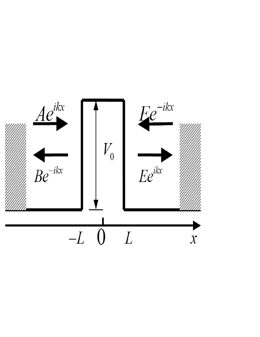
Figure 1: Schematic demonstration of a single-barrier tunneling problem. The quantum states between two reservoirs at zero bias is indicated.

We start with the wave function picture and consider an electron tunneling through a one-dimensional single barrierRef29 , which can be realized in a semiconductor heterostructure with a layer of ${\rm{Al}}_{x}{\rm{Ga}}_{1-x}{\rm{As}}$ of width $2L$ imbedded in $\rm{GaAs}$ as shown in Fig. 1. In the effective mass approximation, the electron motion in each layer of the structure is described by the stationary solution of the envelop equation in the $x$-direction.

$$\left[{\frac{{-\hbar^{2}}}{2}\frac{\partial}{{\partial x}}\frac{1}{{m^{*}\left(x\right)}}\frac{\partial}{{\partial x}}+V_{eff}\left(x\right)}\right]\psi\left(x\right)=E\psi\left(x\right).$$ (1)

Here, $m^{*}$ and $V_{eff}$ are the effective mass and potential in different regions with $E$ the energy of the transporting electron. The electron’s wave functions are expressible as

$$\Psi\left({x,t}\right)=\psi\left(x\right)e^{-iEt/\hbar}=\left\{\begin{array}[]{l}\begin{array}[]{*{20}c}{\left({Ae^{ikx}+Be^{-ikx}}\right)e^{-iEt/\hbar},}&{x\leq-L,}\\ \end{array}\\ \begin{array}[]{*{20}c}{\left({Ce^{\kappa x}+De^{-\kappa x}}\right)e^{-iEt/\hbar},}&{-L\leq x\leq L}\\ \end{array},\\ \begin{array}[]{*{20}c}{\left({Ee^{ikx}+Fe^{-ikx}}\right)e^{-iEt/\hbar},}&{x\geq L,}\\ \end{array}\\ \end{array}\right.$$ (2)

with $k={{\sqrt{2m^{*}E}}\mathord{\left/{\vphantom{{\sqrt{2m^{*}E}}\hbar}}\right.\kern-1.2pt}\hbar}$ and $\kappa={{\sqrt{2m^{*}\left({V_{0}-E}\right)}}\mathord{\left/{\vphantom{{\sqrt{2m^{*}\left({V_{0}-E}\right)}}\hbar}}\right.\kern-1.2pt}\hbar}$. The coefficients $A$ and $B$ are associated respectively with incoming and outgoing waves on the left side relative to the barrier. Likewise, the coefficients $E$ and $F$ are respectively outgoing and incoming waves on the right. The scattering matrix connects the incoming and outgoing fluxes as

$$\left[{\begin{array}[]{*{20}c}B\\ E\\ \end{array}}\right]=\left[{\begin{array}[]{*{20}c}{S_{11}}&{S_{12}}\\ {S_{21}}&{S_{22}}\\ \end{array}}\right]\left[{\begin{array}[]{*{20}c}A\\ F\\ \end{array}}\right].$$ (3)

Ideal (i.e., without scattering) conducting leads connect the scattering region to reservoirs on the left and right characterized by quasi-Fermi energies $\mu_{1}$ and $\mu_{2}$, respectively, corresponding to the electron densities there. These reservoirs or contacts randomize the phase of the injected and absorbed electrons through inelastic processes such that there is no phase relation between particles. For such an ideal 1D system, the current injected from the left and right may be written as an integral over the fluxRef29 ; Ref33

$$I_{L}=\frac{{2e}}{{2\pi}}\left[{\int_{0}^{\infty}{dkv\left(k\right)f_{1}\left(k\right)T\left(E\right)}-\int_{0}^{\infty}{dk^{\prime}v\left({k^{\prime}}\right)f_{2}\left({k^{\prime}}\right)T\left({E^{\prime}}\right)}}\right],$$ (4)

where $v(k)$ is the velocity, $T(E)$ is the transmission coefficient, which can be obtained from the wave function Eq. (2), and $f_{1}$ and $f_{2}$ are the reservoir distribution functions characterized by $\mu_{1}$ and $\mu_{2}$, respectively. The integrations are only over positive $k$ and $k^{\prime}$ relative to the direction of the injected charge as positive $k$ is in $+x$-direction and positive $k^{\prime}$ is in $-x$-direction. If we now assume low temperatures, electrons are injected up to an energy $\mu_{1}$ from the left lead and injected up to $\mu_{2}$ from the right one. Converting to integrals over energy, the current becomes

$$\begin{array}[]{l}I_{L}=\frac{{2e}}{{2\pi}}\left[{\int_{0}^{\mu_{1}}{dE\left({\frac{{dk}}{{dE}}}\right)v\left(k\right)T\left(E\right)}-\int_{0}^{\mu_{2}}{dE\left({\frac{{dk^{\prime}}}{{dE}}}\right)v\left({k^{\prime}}\right)T\left(E\right)}}\right]\\ =\frac{{2e}}{{2\pi\hbar}}\int_{\mu_{2}}^{\mu_{1}}{dET\left(E\right)}.\\ \end{array}$$ (5)

It can be seen that the first term of Eq. (5) is the flux generated by electrons injected from the left reservoir and the second term is that from the right reservoir. The integration is done in two independent ensembles.

The Landauer-Büttiker conductance introduced above can be reproduced in the second-quantization language. Without loss of generality, we assume the input amplitudes from the two reservoirs in Eq. (2) to be unity. For simplicity, as a single channel is considered, the scattering matrix can be described in the relation

$$\hat{b}_{\alpha}=S_{\alpha\beta}\hat{a}_{\beta}$$ (6)

or elaborately

$$\left[{\begin{array}[]{*{20}c}{\hat{b}_{L}}\\ {\hat{b}_{R}}\\ \end{array}}\right]=\left[{\begin{array}[]{*{20}c}{S_{11}}&{S_{12}}\\ {S_{21}}&{S_{22}}\\ \end{array}}\right]\left[{\begin{array}[]{*{20}c}{\hat{a}_{L}}\\ {\hat{a}_{R}}\\ \end{array}}\right]=\left[{\begin{array}[]{*{20}c}r&{t^{\prime}}\\ t&{r^{\prime}}\\ \end{array}}\right]\left[{\begin{array}[]{*{20}c}{\hat{a}_{L}}\\ {\hat{a}_{R}}\\ \end{array}}\right],$$ (7)

where operators $a_{L/R}$ annihilate electrons incident upon the sample from the left/right reservoir and operators $b_{L/R}$ describe electrons in the outgoing states. $t$ and $t^{\prime}$ are the transmission amplitudes of electrons incident rightward and rightward, respectively, and $r$ and $r^{\prime}$ are the corresponding reflection amplitudes, as defined conventionally. Hence, the Landauer-Büttiker formula of the current can be expressed as

$$I_{L}=\frac{e}{{2\pi\hbar}}\int{dE\left\langle{\left[{a_{L}^{\dagger}\left(E\right)a_{L}\left(E\right)-b_{L}^{\dagger}\left(E\right)b_{L}\left(E\right)}\right]}\right\rangle},$$ (8)

where $\left\langle\cdots\right\rangle$ calculates the quantum statistical average of the product of an electron creation operator and annihilation operator of a Fermi gas. As a conventional electron reservoir is considered, we have

$$\begin{array}[]{l}\left\langle{a_{L}^{\dagger}\left(E\right)a_{L}\left({E^{\prime}}\right)}\right\rangle=f_{L}\left(E\right)\delta\left({E-E^{\prime}}\right),\\ \left\langle{a_{R}^{\dagger}\left(E\right)a_{R}\left({E^{\prime}}\right)}\right\rangle=f_{R}\left(E\right)\delta\left({E-E^{\prime}}\right),\\ \left\langle{a_{L}^{\dagger}\left(E\right)a_{R}\left({E^{\prime}}\right)}\right\rangle=\left\langle{a_{R}^{\dagger}\left(E\right)a_{L}\left({E^{\prime}}\right)}\right\rangle=0.\\ \end{array}$$ (9)

It should be noted from the third formula of Eq. (9) that electrons incident from the left and right reservoirs are completely incoherent and the phases of the two reservoirs are randomized and completely unrelated. Substituting Eq. (9) to Eq. (8), the formula of the current expressed in Eq. (5) can be reproduced.

It is interesting to see that if we could build up a system with the conductor connected to two correlated reservoirs, in which the quantum statistical average of the cross product reads

$$\begin{array}[]{l}\left\langle{a_{L}^{\dagger}\left(E\right)a_{R}\left({E^{\prime}}\right)}\right\rangle=\left\langle{a_{R}^{\dagger}\left(E\right)a_{L}\left({E^{\prime}}\right)}\right\rangle=f_{3}\left(E\right)\delta\left({E-E^{\prime}}\right),\\ f_{3}\left(E\right)=\left\{\begin{array}[]{l}1,\begin{array}[]{*{20}c}{}\hfil&{\mu<\min\left({\mu_{1},\mu_{2}}\right),}\\ \end{array}\\ 0,\begin{array}[]{*{20}c}{}\hfil&{{\rm{others}},}\\ \end{array}\\ \end{array}\right.\\ \end{array}$$ (10)

the system can generate a current demonstrating the interference between the electron states incident from the left reservoir and the right one.

$$I_{L}=-\frac{e}{{2\pi\hbar}}\int_{0}^{\mu_{1}}{dE}\left[{\int_{0}^{\mu_{1}}{\left|r\right|^{2}dE}+\int_{0}^{\mu_{2}}{\left|t\right|^{2}dE}+2\int_{0}^{\mu\left({\min}\right)}{{\mathop{\rm Re}\nolimits}\left({r^{*}t^{\prime}}\right)dE}}\right].$$ (11)

In the next subsection, we would use a toy system based on correlated reservoirs to further illustrate the scattering scheme. Significant difference between uncorrelated and correlated reservoirs is illuminated. It is also elaborated that in scattering problems the transmission and reflection process demonstrates the quantum state spanned throughout the space.

I.2 Further illustration of the scattering scheme in a toy system with correlated reservoirs

We consider incidence only from the left in Eq. (2) and the input flux is assumed to be unity. The wave function in different scattering regions can be expressed as

$$\psi\left(x\right)=\left\{\begin{array}[]{l}\begin{array}[]{*{20}c}{e^{ikx}+re^{-ikx},}&{x\leq-L,}\\ \end{array}\\ \begin{array}[]{*{20}c}{Ce^{\kappa x}+De^{-\kappa x},}&{-L\leq x\leq L}\\ \end{array},\\ \begin{array}[]{*{20}c}{te^{ikx},}&{x\geq L.}\\ \end{array}\\ \end{array}\right.$$ (12)

An incident particle is transmitted with probability $\left|t\right|^{2}$ and reflected with probability $\left|r\right|^{2}$. It is determined by the wave function that the particle momentum has value of $\hbar k$ with probability ${{\left({1+\left|t\right|^{2}}\right)}\mathord{\left/{\vphantom{{\left({1+\left|t\right|^{2}}\right)}2}}\right.\kern-1.2pt}2}$ and $-\hbar k$ with probability ${{\left|r\right|^{2}}\mathord{\left/{\vphantom{{\left|r\right|^{2}}2}}\right.\kern-1.2pt}2}$. The mean value of the momentum $\left|t\right|^{2}\hbar k$ characterizes the density of the probability current $\bf{J}$, which can also be obtained from the continuity equation ${{\partial\rho}\mathord{\left/{\vphantom{{\partial\rho}{\partial{\rm{t}}}}}\right.\kern-1.2pt}{\partial{\rm{t}}}}+\nabla\cdot{\bf{J}}=0$ with $\rho$ the probability density.

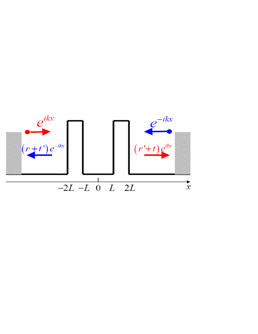
Figure 2: Schematic demonstration of a quantum wire modulated by two potential barriers. The quantum state between two reservoirs at zero bias is indicated.

An interesting interference pattern can be observed if we consider the incidence from the left and the right is correlated. We consider a toy system of a one-dimensional electron gas subject to two oscillating gate volatages (see Fig. 2). The inspiration comes from the quantum pumping phenomenon. The single-particle Hamiltonian reads

$$H=-\frac{\hbar}{{2m^{*}}}\frac{{\partial^{2}}}{{\partial x^{2}}}+U\left({x,t}\right),$$ (13)

with $U\left({x,t}\right)=\Theta\left({x+2L}\right)\Theta\left({-L-x}\right)U_{1}\left(t\right)+\Theta\left({x-L}\right)\Theta\left({2L-x}\right)U_{2}\left(t\right).$ The two barriers $U_{1}$ and $U_{2}$ are adiabatically modulated at the frequency $\omega$ with a phase difference $\phi$.

$$\begin{array}[]{l}U_{1}\left(t\right)=U_{10}+U_{1\omega}\sin\omega t,\\ U_{2}\left(t\right)=U_{20}+U_{2\omega}\sin\left({\omega t-\phi}\right).\\ \end{array}$$ (14)

We assume $\omega$ is extremely small so that a static treatment is valid. Therefore, it is tolerable to consider only the zero order of the Fourier component of the time-dependent scattering matrix without taking into account the photon-absorption/emmission processes, which is done in adiabatic quantum pumping theory.

As shown in Fig. 2, the electrons are incident from the left and right reservoirs with identical amplitudes at zero bias, which is set to be unity without impairing generality. As assumed, incidence from the two correlated reservoirs characterize a coherent single-particle state. The single-particle wave function at a certain time has the following form.

$$\Psi\left({x,t}\right)=\left\{\begin{array}[]{l}\begin{array}[]{*{20}c}{\left[{e^{ikx}+\left({r+t^{\prime}e^{i\theta}}\right)e^{-ikx}}\right]e^{{{-iEt}\mathord{\left/{\vphantom{{-iEt}\hbar}}\right.\kern-1.2pt}\hbar}},}&{x\leq-2L,}\\ \end{array}\\ \begin{array}[]{*{20}c}{\left[{A_{2}e^{\kappa_{2}x}+B_{2}e^{-\kappa_{2}x}}\right]e^{{{-iEt}\mathord{\left/{\vphantom{{-iEt}\hbar}}\right.\kern-1.2pt}\hbar}},}&{-2L\leq x\leq-L}\\ \end{array},\\ \begin{array}[]{*{20}c}{\left[{A_{3}e^{ikx}+B_{3}e^{-ikx}}\right]e^{{{-iEt}\mathord{\left/{\vphantom{{-iEt}\hbar}}\right.\kern-1.2pt}\hbar}},}&{-L\leq x\leq L}\\ \end{array},\\ \begin{array}[]{*{20}c}{\left[{A_{4}e^{\kappa_{4}x}+B_{4}e^{-\kappa_{4}x}}\right]e^{{{-iEt}\mathord{\left/{\vphantom{{-iEt}\hbar}}\right.\kern-1.2pt}\hbar}},}&{L\leq x\leq 2L}\\ \end{array},\\ \begin{array}[]{*{20}c}{\left[{\left({t+r^{\prime}e^{i\theta}}\right)e^{ikx}+e^{-ikx}}\right]e^{{{-iEt}\mathord{\left/{\vphantom{{-iEt}\hbar}}\right.\kern-1.2pt}\hbar}},}&{x\geq 2L.}\\ \end{array}\\ \end{array}\right.$$ (15)

$k={{\sqrt{2m^{*}E}}\mathord{\left/{\vphantom{{\sqrt{2m^{*}E}}\hbar}}\right.\kern-1.2pt}\hbar}$ and $\kappa_{2/4}={{\sqrt{2m^{*}\left({U_{1/2}-E}\right)}}\mathord{\left/{\vphantom{{\sqrt{2m^{*}\left({U_{1/2}-E}\right)}}\hbar}}\right.\kern-1.2pt}\hbar}$. $t$ and $r$ quantify the transmission and reflection amplitudes of the electrons incident from the left reservoir while $t^{\prime}$ and $r^{\prime}$ quantify those incident from the right with $t^{\prime}=t$ and $r^{\prime}={{-tr^{*}}\mathord{\left/{\vphantom{{-tr^{*}}{t^{*}}}}\right.\kern-1.2pt}{t^{*}}}$ . We introduce a geometric phase $\theta$ to describe the unavoidable phase difference between the electrons injected from the two reservoirs. In the toy approach, correlated reservoirs are assumed, which justifies a particular value of $\theta$. For simplicity and without violation of the physics we take $\theta=0$. It is noted that in conventional real reservoirs mixed-ensemble integral should be applied, i.e., the probability flow of the electron incident from the left reservoir absolutely cancels out that of the incidence backward at zero bias as a result of the randomized phase distribution, which absolutely differs from our toy consideration.

From the continuity equation

$$\frac{{\partial\rho}}{{\partial t}}+\nabla\cdot{\bf{J}}=0,$$ (16)

we could derive the probability current flow as functions of the transmission and reflection amplitudes as

$$j_{x}=-\frac{{i\hbar}}{{2m}}\left[{\psi^{\dagger}\frac{\partial}{{\partial x}}\psi-\left({\frac{\partial}{{\partial x}}\psi^{\dagger}}\right)\psi}\right]=-\frac{{4\hbar k}}{m}{\mathop{\rm Re}\nolimits}\left({r^{*}t^{\prime}}\right).$$ (17)

We can also see from the wave function Eq. (15) that the particle momentum has value of $\hbar k$ with probability ${{\left[{1-{\mathop{\rm Re}\nolimits}\left({tr^{*}}\right)}\right]}\mathord{\left/{\vphantom{{\left[{1-{\mathop{\rm Re}\nolimits}\left({tr^{*}}\right)}\right]}2}}\right.\kern-1.2pt}2}$ and $-\hbar k$ with probability ${{\left[{1+{\mathop{\rm Re}\nolimits}\left({tr^{*}}\right)}\right]}\mathord{\left/{\vphantom{{\left[{1+{\mathop{\rm Re}\nolimits}\left({tr^{*}}\right)}\right]}2}}\right.\kern-1.2pt}2}$. The mean value of the momentum $-{\mathop{\rm Re}\nolimits}\left({tr^{*}}\right)\hbar k$ characterizes the density of the probability current of Eq. (17). The net current density can be described by the period-average of the probability current density multiplied by the carrier charge and density. The accumulated contribution by electrons within the $\pm\hbar\omega$ sidebands is taken into account by an integral. Without dynamic modulation, no current occurs as the $\pm\hbar\omega$ energy channel is closed even when the probability current density is nonzero for asymmetric barrier configuration. The current density as a function of the Fermi level thus becomes

$$I_{L}\left(E_{F}\right)=-\frac{{4\hbar}}{{m^{*}}}\int_{E_{F}-\hbar\omega}^{E_{F}+\hbar\omega}{\frac{{ek\rho_{e}N\left(E\right)f\left(E\right)}}{{\left({{{2\pi}\mathord{\left/{\vphantom{{2\pi}\omega}}\right.\kern-1.2pt}\omega}}\right)}}\int_{0}^{\frac{{2\pi}}{\omega}}{{\mathop{\rm Re}\nolimits}\left[{r^{*}\left(t\right)t^{\prime}\left(t\right)}\right]dt}dE},$$ (18)

where the density of states of a one-dimensional electron gas is

$$N\left(E\right)=\frac{V}{{\pi\hbar}}\sqrt{\frac{{m_{e}}}{{2E}}}.$$ (19)

Here, $k$ is the wave vector of the electron. $e$ is the electron charge. $\rho_{e}$ is the carrier density of the two-dimensional electron gas in which the quantum wire is confined. $f(E)$ is the Fermi-Dirac distribution function of the leads. $V$ quantifies the volume of the one-dimensional wire and $m_{e}$ is the mass of a free electron.

Here, in the toy configuration, quantum interference is remarkably demonstrated. The single-electron state Eq. (15) interferes with itself and carries the probability flow and hence the net current through oscillating cycles.

We numerically calculated the current in a one-dimensional electron gas (2DEG) based on the GaAs/AlGaAs heterostructures with the average carrier density $\rho_{e}\sim 10^{11}$ cm^-2 and the effective mass of the electron $m^{*}\sim 0.067m_{e}$Ref73 . The width of the two gate potential barriers $L=20$ Å equally separated by a $2L=40$ Å width well. The amplitudes of the modulations $U_{1\omega}=U_{2\omega}=1$ meV. All of the above setups are not essential as we are dealing with an assumed toy structure.

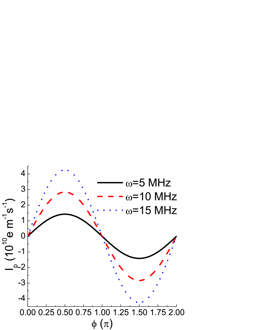
Figure 3: Time-integrated current density as a function of the phase difference between the two modulations for different modulation frequencies. The Fermi level of the two reservoirs $E_{F}=60$ meV counting from the conduction band edge of the electron gas structure.

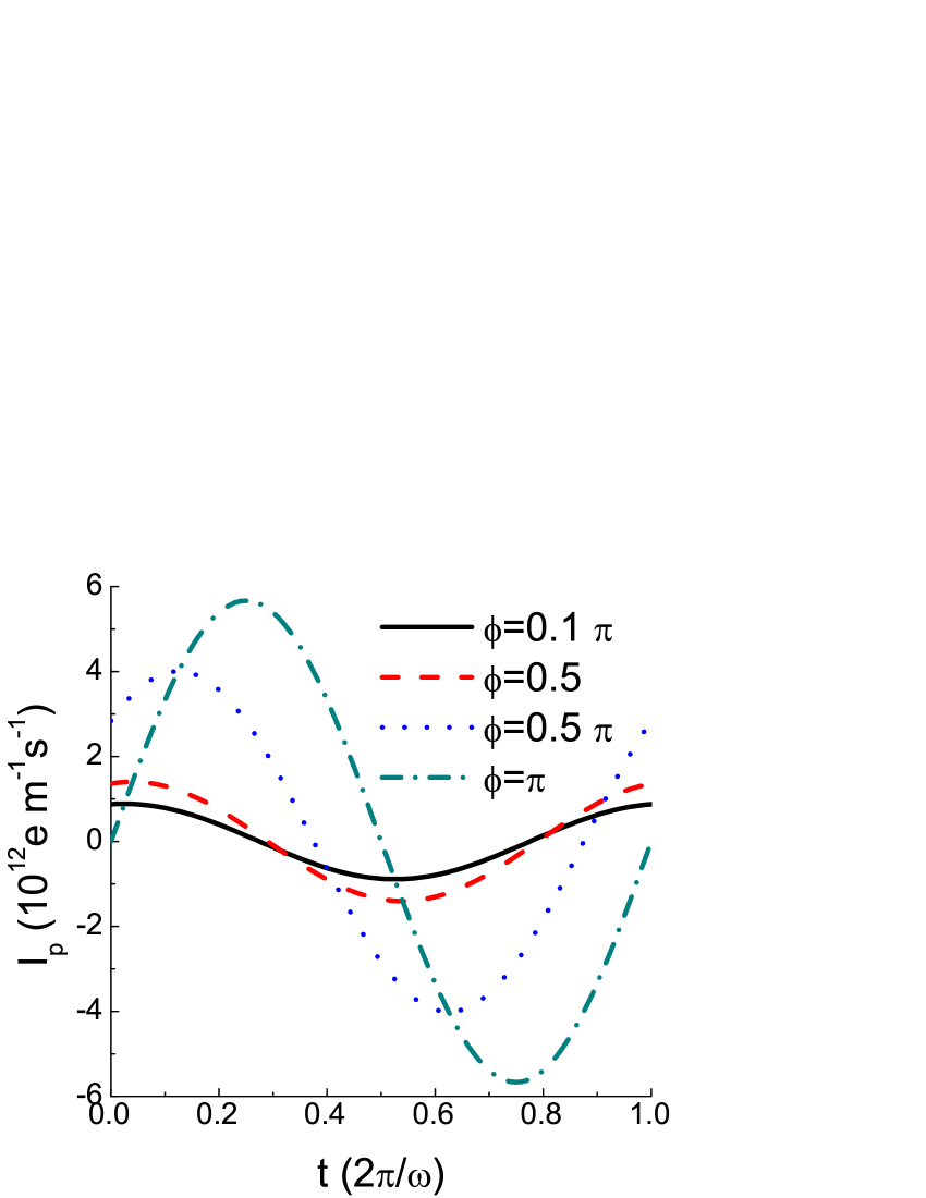
Figure 4: Time variation of the current density within an oscillating cycle. Different phase difference between the two modulations is considered. The modulation frequency is set to be $\omega=10$ MHz and the Fermi level $E_{F}$ to be 60 meV.

In Fig. 3, it is shown that the time-integrated current demonstrates a sinusoidal pattern as a function of the phase difference between two oscillating parameters, which is a result of quantum interference. The probability density flow formulated in Eq. (17) is a result of phase difference between transmission forward and backward. Quantum phase interference gives rise to nonzero probability density flow for asymmetric barrier configurations. The absolute strength of the probability flow increases as the height difference between the two potential barriers increases determined by the phase difference $\phi$. Fig. 4 presented the time variation of the net current within an oscillating cycle. Considering the time-averaged effect, the integrated asymmetry is different. When the phase difference between the two modulations approaches $\pi$, time-reversal symmetry destroys the time-integrated current to zero although the probability density flow maximizes at a certain time. i.e. the probability flow in half a pumping cycle completely offsets that of the other. Therefore a sinusoidal dependence on $\phi$ occurs in the time-integrated current.

In real reservoirs, the single-particle state between reservoirs has a definite momentum direction determined by its source. When coherent reservoirs can be realized in any form, however, quantum states within the mesoscopic conductor can be expressed as Eq. (15) and double-slit interference pattern is observable in an electron device.

I.3 Time-dependent scattering-matrix theory

The scattering-matrix equation $\hat{b}_{\alpha}=S_{\alpha\beta}\hat{a}_{\beta}$ with $\alpha$ and $\beta$ indexes of lead, channel, and spin introduced in Sec. I.A. for the Landauer-Büttiker conductance characterizes the transport properties through a conductor at a certain bias.

In a more general situation with dynamic processes, e.g. in quantum pumping, a time-dependent scattering matrix can be introduced as follows.

$$\hat{b}_{\alpha}\left(t\right)=\int_{-\infty}^{\infty}{S_{\alpha\beta}\left({t,t^{\prime}}\right)\hat{a}_{\beta}\left({t^{\prime}}\right)dt^{\prime}},\begin{array}[]{*{20}c}{}\hfil&{t\geq t^{\prime},}\\ \end{array}$$ (20)

with $\alpha$ and $\beta$ general indexes denoting the lead, channel, and spin. An incident state $\hat{a}_{\beta}$ at time $t^{\prime}$ is scattered into the outgoing state $\hat{b}_{\alpha}$ at time $t$ with the amplitude $S_{\alpha\beta}\left({t,t^{\prime}}\right)$.

The time-dependent scattering-matrix picture described by Eq. (20) is exactly equivalent to the time-dependent Schrödinger equation with the elements of the scatting matrix amplitudes of the wave function. In usual cases, the time-dependent Schrödinger equation cannot be solved exactly, similarly to the time-dependent scattering matrix. In the static or adiabatic cases, it is advantageous to use an analog of the Wigner transform for the matrix $S_{\alpha\beta}\left({t,t^{\prime}}\right)$trs ,

$$S_{\alpha\beta}\left({E,t}\right)=\int_{-\infty}^{\infty}{e^{iE\left({t-t^{\prime}}\right)}S_{\alpha\beta}\left({t,t^{\prime}}\right)dt^{\prime}}.$$ (21)

An on-time scattering process $S_{\alpha\beta}\left({t,t^{\prime}}\right)$ with $t=t^{\prime}$ is sufficient to describe the bias-driven conductance. Namely, from Eq. (21), we can use $S_{\alpha\beta}\left({E}\right)$ with $E$ labeling the energy channel to fully capture the transport physics.

When the scattering time $t-t^{\prime}$ is small (i.e., the dynamic characteristic frequency is much smaller than the inverse Wigner time delay), the dynamics can be approximated into the instant-scattering picture. Physically this means that the scattering matrix changes only a little while an electron is scattered by the mesoscopic sample under dynamic modulation, in which we use the term “adiabatic”. In adiabatic dynamics, we can use low-order Fourier components of $S_{\alpha\beta}\left({E,t}\right)$ to characterize transport physics. Therefore, small $t-t^{\prime}$ is transformed into variation of the particle energy by side-band broadening around the Fermi level.

In Sec. III, we would illustrate the time-dependent scattering approach in adiabatic quantum pumping beyond the linear-response approximation.

II Spin-orbit coupling affected shot noise

II.1 Background

Current fluctuations are present in almost all kinds of conductors and have been developed into a very active and fascinating subfield of mesoscopic physics (for review see Ref. Ref20, ). At low temperatures, thermal fluctuations are extremely small, the current fluctuation properties are governed by the so-called shot noise, which is a consequence of the quantization of charge. Shot noise is useful to obtain information on a system which is not available through conductance measurements. In particular, shot noise experiments can determine the quantum correlation of electrons, the charge and statistics of the quasi-particles relevant for transport, and reveal information on the potential profile as well as internal energy scales of mesoscopic systemsRef34 ; Ref35 ; Ref36 ; Ref37 ; Ref38 ; Ref39 ; Ref40 ; Ref41 ; Ref42 ; Ref43 ; Ref44 ; Ref45 ; Ref22 ; Ref60 . Shot noise is generally more sensitive to the effects of electron-electron interactions than the average conductance.

A convenient measure of shot noise is the Fano factor $F$, which is the ratio of the actual shot noise and the Poisson noise. The Poisson noise would be achieved in measurement if the transport is carried by single independent electrons. Four typical values of the Fano factor characterize the shot noise properties of different mesoscopic conductors.

1. $F=1$ characterizes Poissonian processes. Particles are completely independent during transport corresponding to channels through which transmission is exponentially small. In diffusive transport, they are the so-called approximately-closed channels. Typical conductors featuring $F=1$ include tunneling junction, Schottky-barrier diode, and asymmetric double-barrier diode.

2. $F=0$ characterizes ballistic transport. In ballistic transport, transmission approaches the maximum of unity. Free particles wave function extends throughout the space, i.e. particle beams exhibit full coherence. In diffusive transport, they are the so-called open channels. Typical conductors featuring $F=0$ include pure metal and free two-dimensional electron gas.

3. $F=1/3$ characterizes diffusive transport. Open channels and closed channels are distributed randomly. As a result of ensemble average of channels, the strength shot noise falls between $F=1$ and $F=0$. Typical conductors featuring $F=1/3$ include diffusive metals, graphene, and two-dimensional electron gas modulated by magnetic barriers.

4. $F=1/2$ characterizes ballistic transport constrained by Pauli principle. The Pauli principle forbids two electrons to be in the same channel simultaneously. As a result, the shot noise is suppressed. All kinds of conductors are subject to the Pauli principle. In the symmetric-double-barrier diode, where Pauli exclusion is the only correlation between particles, the shot noise features $F=1/2$.

With increased attentionRef46 ; Ref47 ; Ref48 ; Ref49 ; Ref50 ; Ref51 to semiconductor spintronics, materials such as ${\rm{GaSb}}$, ${\rm{InAs}}$, and ${\rm{InSb}}$ with considerably strong spin-orbit coupling (SOC) constantRef51 ; Ref52 are becoming widely used in mesoscopic conductors, observationsRef34 ; Ref37 ; Ref38 beyond the formalism of earlier theory on current shot noise are reported. The scattering approach is developed to derive a general formula for the shot noise in the presence of the SOC effect and apply it to the double-barrier resonant diode (DBRD) systems. It is demonstrated that the microscopic origin of the super-suppression of the shot noise observed in experimentRef34 ; Ref37 ; Ref38 is the bunching interaction between electrons with opposite spins resulting from the Dresselhaus $k^{3}$ termsRef53 ; Ref54 in the effective Hamiltonian of the bulk semiconductor of the barriers.

II.2 Theoretical approach

In this part, the effect of the Dresselhaus SOC to the shot noise properties in the DBRD structure connected to ferromagnetic or normal metal leads is considered. The theory can be generalized to other coherent mesoscopic conductors subject to Dresselhaus and/or Rashba SOC.

The Dresselhaus SOC is caused by the bulk inversion asymmetry and exists broadly in III-V compound semiconductors with zinc-blende crystal structuresRef53 . Consider the transmission of electrons with identical wave vector ${\bf{k}}=({\bf{k}}_{\parallel},k_{z})$ through a certain potential barrier grown along $z\parallel[001]$ direction. ${\bf{k}}_{\parallel}$ is the wave vector in the plane of the barrier and $k_{z}$ is the wave vector component normal to the barrier. The electron Hamiltonian of the barrier in the effective-mass approximation contains the spin-dependent $k^{3}$ Dresselhaus term

$$\hat{H}_{D}=\gamma(\hat{\sigma}_{x}k_{x}-\hat{\sigma}_{y}k_{y})\frac{{\partial^{2}}}{{\partial z^{2}}},$$ (22)

where $\gamma$ is the material constant denoting the strength of the Dresselhaus SOC, $\hat{\sigma}_{x}$ and $\hat{\sigma}_{y}$ are the Pauli matrices. The Dresselhaus term can be diagonalized by the spinors

$$\chi_{\pm}=\frac{1}{{\sqrt{2}}}\left({\begin{array}[]{*{20}c}1\\ {\mp e^{-i\varphi}}\\ \end{array}}\right),$$ (23)

which describe the spin-up (“$+$”) and spin-down (“$-$”) electron eigenstates.

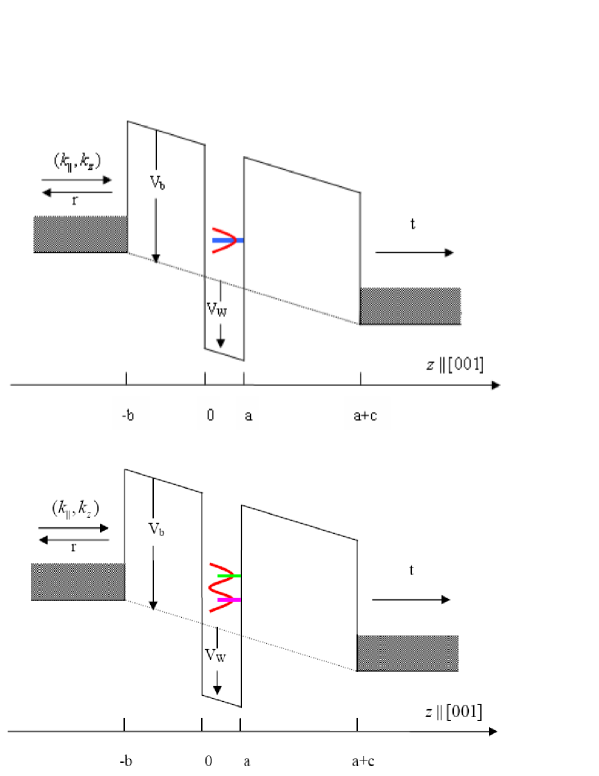
Figure 5: Schematics of the double-barrier resonant diode. The resonant level is sketched between the two barriers. The upper panel demonstrates the resonant level in conventional diode without the spin-orbit coupling (SOC). In the lower panel, the SOC behaves like a pseudomagnetic field and induces a split of different spin components of the resonant level in the barrier structure, which contribute collectively to the electric current and shot noise.

Suppose the system is a layered mesoscopic conductor with its potential profile described by $V_{0}(z)$ (see Fig. 5), the electron motion in each layer of the structure is described by the Hamiltonian

$$\hat{H}=-\frac{{\hbar^{2}}}{{2m^{*}}}\nabla^{2}+V(z)+\hat{H}_{D},$$ (24)

where $V(z)=V_{0}(z)-eF(z+b)\Theta(z+b)\Theta(a+c-z)$ with $F$ the magnitude of the electric field, $\Theta(z)$ the step function, and $-b$ and $a+c$ the longitudinal coordinates of surfaces in $z$ direction. Our discussion is within the framework of single electron approximation and coherent tunnelingRef55 ; Ref56 , and only zero-frequency noise at zero temperature is considered. Under the assumption that $k_{\parallel}$ is conserved during the tunneling, the wave functions for the electrons with definite longitudinal electron energy ($E_{z}$) can be obtained from Schrödinger equation based on the Hamiltonian given in Eq. (24), which can be diagonalized by spinors $\chi_{\pm}$. So, the wave functions become

$$\psi(\mathord{\buildrel{\lower 3.0pt\hbox{$\scriptscriptstyle\rightharpoonup$}}\over{r}})=\left\{{\begin{array}[]{*{20}c}{\exp(i{\bf{k}}_{\parallel}\cdot{\bf{\rho}})\left({\sum\limits_{j=\pm}{\sqrt{\frac{{m_{1}}}{{\hbar k_{1j}}}}\exp(ik_{1j}z)\chi_{j}}+\sum\limits_{j=\pm}{r_{j}\sqrt{\frac{{m_{1}}}{{\hbar k_{1j}}}}\exp(-ik_{1j}z)\chi_{j}}}\right),}&{z<b,}\\ {\exp(i{\bf{k}}_{\parallel}\cdot{\bf{\rho}})\sum\limits_{j=\pm}{\Phi_{\xi j}(z)},}&{-b\leq z<a+c,}\\ {\exp(i{\bf{k}}_{\parallel}\cdot{\bf{\rho}})\sum\limits_{j=\pm}{t_{j}\sqrt{\frac{{m_{5}}}{{\hbar k_{5j}}}}\exp(ik_{5j}z)\chi_{j}},}&{z\geq a+c,}\\ \end{array}}\right.$$ (25)

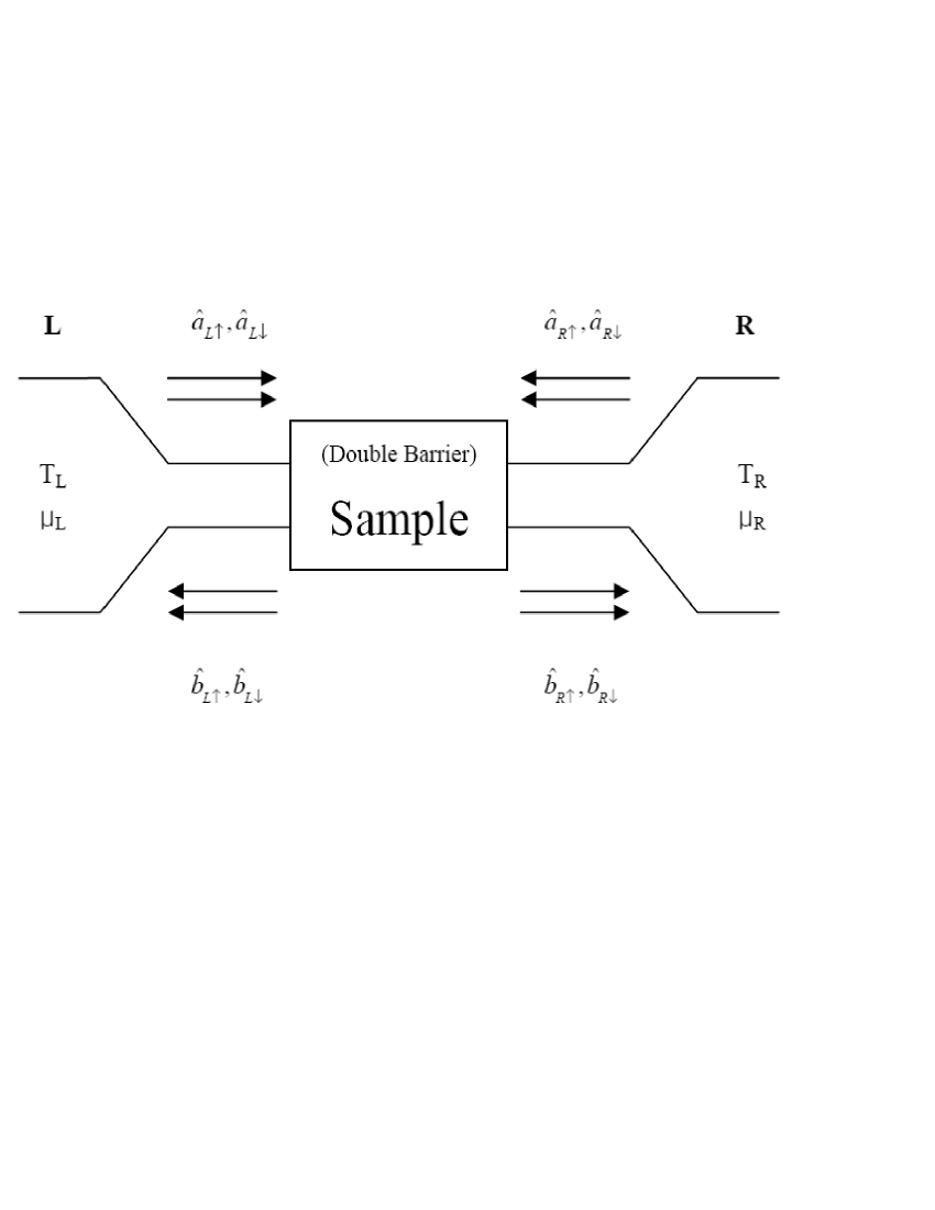
Figure 6: Schematics of the scattering approach. Spin components of the incoming and outgoing states are indicated.

where $\Phi_{\xi j}$ denotes the wave function in the conductor region, and $t_{j}$ and $r_{j}$ are the transmission and reflection amplitudes, which can be calculated using the transfer-matrix methodRef57 . The spin “$+$” and spin “$-$” components of the electron wave functions transport separately without correlation. As standard scattering method is applied, we introduce creation and annihilation operators of electrons in the scattering states. Schematics of the scattering states are shown in Fig. 6. Operators $\hat{a}_{Ln\sigma}^{\dagger}(E)$ and $\hat{a}_{Ln\sigma}(E)$ create and annihilate electrons with total energy $E$ and spin polarization $\sigma$ in the transverse channel $n$ in the left lead, which are incident upon the sample. In the same way, the creation $\hat{b}_{Ln\sigma}^{\dagger}(E)$ and annihilation $\hat{b}_{Ln\sigma}(E)$ operators describe electrons in the outgoing states. They obey anti-commutation relations. Therefore, we can write the scattering matrix of the sample as

$$\begin{array}[]{c}\left({\begin{array}[]{*{20}c}{\hat{b}_{Ln\uparrow}}\\ {\hat{b}_{Ln\downarrow}}\\ {\hat{b}_{Rn\uparrow}}\\ {\hat{b}_{Rn\downarrow}}\\ \end{array}}\right)=\frac{1}{2}\underbrace{\left({\begin{array}[]{*{20}c}1&1&0&0\\ {e^{-i\varphi}}&{-e^{-i\varphi}}&0&0\\ 0&0&1&1\\ 0&0&{e^{-i\varphi}}&{-e^{-i\varphi}}\\ \end{array}}\right)}_{M_{1}}\times\underbrace{\left({\begin{array}[]{*{20}c}{r_{+}}&0&{t_{+}^{\prime}}&0\\ 0&{r_{-}}&0&{t_{-}^{\prime}}\\ {t_{+}}&0&{r_{+}^{\prime}}&0\\ 0&{t_{-}}&0&{r_{-}^{\prime}}\\ \end{array}}\right)}_{s}\\ \times\underbrace{\left({\begin{array}[]{*{20}c}1&{-e^{i\varphi}}&0&0\\ 1&{e^{i\varphi}}&0&0\\ 0&0&1&{-e^{i\varphi}}\\ 0&0&1&{e^{i\varphi}}\\ \end{array}}\right)}_{M_{2}}\times\left({\begin{array}[]{*{20}c}{\hat{a}_{Ln\uparrow}}\\ {\hat{a}_{Ln\downarrow}}\\ {\hat{a}_{Rn\uparrow}}\\ {\hat{a}_{Rn\downarrow}}\\ \end{array}}\right),\\ \end{array}$$ (26)

with $t^{\prime}=t,r^{\prime}=-\frac{t}{{t^{*}}}r^{*}$, $T_{j}(E)=\left|{t_{j}}\right|^{2},R_{j}(E)=\left|{r_{j}}\right|^{2}$, and $j=\pm$. The matrices $M_{1}$ and $M_{2}$ are unitary transformations between spin “$\uparrow\downarrow$” states and spin “$\pm$” states, $s$ is the scattering matrix connecting the incoming and outgoing spin “$\pm$” states of the $n$th channel. The current of the system can be derived as follows

$$\hat{I}_{L}(t)=\frac{e}{{2\pi\hbar}}\sum\limits_{\alpha\beta}{\sum\limits_{mn}{\sum\limits_{\sigma^{\prime}\sigma^{\prime\prime}}{\sum\limits_{\sigma}{\int{dE}\int{dE^{\prime}}e^{i(E-E^{\prime})t/\hbar}\hat{a}_{\alpha m\sigma^{\prime}}^{\dagger}}}}}(E)A_{\alpha,\beta,\sigma^{\prime},\sigma^{\prime\prime}}^{m,n,\sigma}(L;E,E^{\prime})\hat{a}_{\beta n\sigma^{\prime\prime}}(E^{\prime}),$$ (27)

where

$$\begin{array}[]{l}A_{\alpha,\beta,\sigma^{\prime},\sigma^{\prime\prime}}^{m,n,\sigma}(L;E,E^{\prime})=\\ \delta_{\alpha L}\delta_{mm}\delta_{\beta L}\delta_{\sigma^{\prime}\sigma}\delta_{\sigma^{\prime\prime}\sigma}-\sum\limits_{\xi^{\prime}\xi^{\prime\prime}}{\sum\limits_{k}{M_{2\xi^{\prime\prime}\sigma^{\prime}}^{\dagger}s_{L,\alpha;m,k;\xi^{\prime\prime}}^{\dagger}}(E)M_{1\sigma\xi^{\prime\prime}}^{\dagger}M_{1\sigma\xi^{\prime}}s_{L,\beta;k,n;\xi^{\prime}}(E^{\prime})M_{2\xi^{\prime}\sigma^{\prime\prime}}}.\\ \end{array}$$ (28)

For a system at thermal equilibrium, the quantum statistical average of the product of an electron creation operator and annihilation operator of a Fermi gas with spin polarization is

$$\begin{array}[]{*{20}c}{\left\langle{a_{Ln\uparrow}^{\dagger}a_{Ln\uparrow}}\right\rangle=f_{Lp},}&{\left\langle{a_{Ln\downarrow}^{\dagger}a_{Ln\downarrow}}\right\rangle=f_{La},}&{\left\langle{a_{Ln\uparrow}^{\dagger}a_{Ln\downarrow}}\right\rangle=\left\langle{a_{Ln\downarrow}^{\dagger}a_{Ln\uparrow}}\right\rangle=\frac{1}{2}(f_{Lp}-f_{La}).}\\ \end{array}$$ (29)

Without loss of generality, we set the unit vector directed along the spin orientation ${\bf{n}}_{s}=(1,0,0)$. Making use of Eqs. (24)-(26), after some algebra, we can obtain the expression for the zero-frequency noise power

$$\begin{array}[]{l}S_{\alpha\beta}\equiv S_{\alpha\beta}(0)=\frac{{e^{2}}}{{4\pi\hbar}}\sum\limits_{\delta\delta_{2}}{\sum\limits_{mn}{\sum\limits_{\scriptstyle\sigma^{\prime}\sigma^{\prime\prime}\hfill\atop\scriptstyle\sigma_{2}^{\prime}\sigma_{2}^{\prime\prime}\hfill}{\sum\limits_{\scriptstyle\sigma\hfill\atop\scriptstyle\sigma_{2}\hfill}{\int{dE}}}}}\\ \times\left\{{A_{\delta,\delta_{2},\sigma^{\prime},\sigma^{\prime\prime}}^{m,n,\sigma}(\alpha;E,E)A_{\delta_{2},\delta,\sigma_{2}^{\prime},\sigma_{2}^{\prime\prime}}^{n,m,\sigma_{2}}(\beta;E,E)+A_{\delta,\delta_{2},\sigma^{\prime},\sigma^{\prime\prime}}^{m,n,\sigma}(\beta;E,E)A_{\delta_{2},\delta,\sigma_{2}^{\prime},\sigma_{2}^{\prime\prime}}^{n,m,\sigma_{2}}(\alpha;E,E)}\right\}\\ \times\left\{{\left[{\delta_{\sigma^{\prime\prime}\sigma_{2}^{\prime}}\delta_{\sigma^{\prime}\sigma_{2}^{\prime\prime}}f_{\delta}(E)+\delta_{\sigma^{\prime\prime}\sigma_{2}^{\prime}}\delta_{\bar{\sigma}^{\prime}\sigma_{2}^{\prime\prime}}\frac{1}{2}\left({f_{p\delta}(E)-f_{a\delta}(E)}\right)}\right]}\right.\\ \left.{-\left[{\delta_{\sigma^{\prime}\sigma_{2}^{\prime\prime}}f_{\delta}(E)+\delta_{\bar{\sigma}^{\prime}\sigma_{2}^{\prime\prime}}\frac{1}{2}\left({f_{p\delta}(E)-f_{a\delta}(E)}\right)}\right]\times\left[{\delta_{\sigma^{\prime\prime}\sigma_{2}^{\prime}}f_{\delta_{2}}(E)+\delta_{\bar{\sigma}^{\prime\prime}\sigma_{2}^{\prime}}\frac{1}{2}\left({f_{p\delta_{2}}(E)-f_{a\delta_{2}}(E)}\right)}\right]}\right\}.\\ \end{array}$$ (30)

Eq. (30) gives a general formula to calculate the shot noise in mesoscopic conductors subject to the SOC effect. It can be used to predict the low-frequency noise properties of arbitrary multi-channel, multi-probe phase-coherent conductors in the presence of Dresselhaus SOC. It can be naturally extended to the system with Rashba SOC and the system with both Dresselhaus SOC and Rashba SOC. In the limit of zero SOC and when the conductor is connected to normal metal leads, there is $f_{\alpha a}(E)=f_{\alpha p}(E)$ and $T_{n+}(E)=T_{n-}(E)=T(E)$, thus Eq. (30) reconverts to the formula provided by BüttikerRef58 concerning scalar electron systems without the spin degree of freedom inducing observable difference.

II.3 Numerical results in comparison with experiment

To further demonstrate our theory, we provide numerical results based on real heterostructures in comparison with experiment.

The double-barrier structure considered here is constructed of layers of ${\rm{Ga}}_{\rm{x}}{\rm{Al}}_{{\rm{1-x}}}{\rm{Sb}}$ with $x=0.15/0.3/0/0.3/0.15$ ($x=0.3$ for the barriers and $x=0$ for the well), which are known to be semiconductors with relatively strong Dresselhaus SOCRef55 ; Ref56 . Our target setup is a symmetric double-barrier structure with the thickness of the well $a=30$ ${\rm{{\AA}}}$ and the thickness of the two barriers $b=c=50$ ${\rm{{\AA}}}$. The height of the barrier $V_{b}=230$ ${\rm{meV}}$ and the depth of the well $V_{w}=200$ ${\rm{meV}}$ are given by the heterostructure propertiesRef57 (cf. Fig. 5). We assume that in the whole region the effective mass $m^{*}=0.053m_{e}$Ref55 ; Ref56 . The chemical potential of the two electrodes is set to be ${\rm{12}}$ ${\rm{meV}}$. For comparison, we choose the Dresselhaus constant $\gamma=0,40,80,120$ ${\rm{eV}}$ ${\rm{{\AA}^{3}}}$.

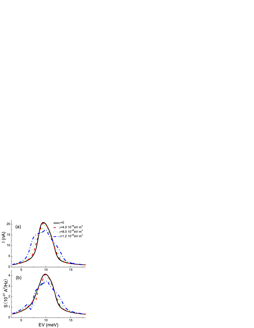
Figure 7: Current $I$ (a) and shot noise $S$ (b) as functions of the applied bias $EV$ of electrons traversing a symmetric DBRD structure with different Dresselhaus constants $\gamma$.

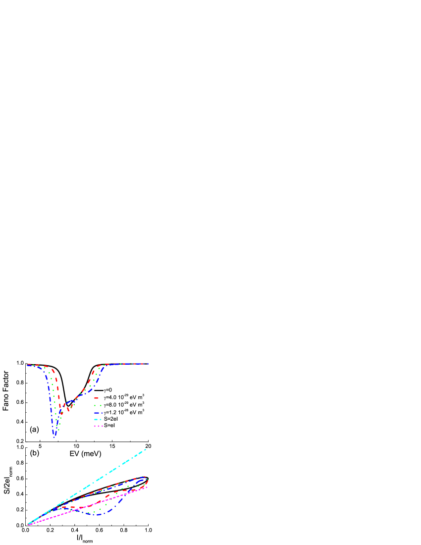
Figure 8: Fano factor as a function of the applied bias $EV$ (a) and $S/2eI_{norm}$ vs $I/I_{norm}$ (b) of electrons traversing a symmetric DBRD structure with different Dresselhaus constants $\gamma$. Two straight lines in (b) show the full shot noise value ($2eI$) and half of its value for comparison.

We see the current fluctuation of the system caused by Dresselhaus SOC. Fig. 7 presents results of the electric current $I$ and the shot noise $S$ versus the external bias. It is demonstrated that the peaks of the current and of the shot noise are lowered as the Dresselhaus constant $\gamma$ increases, and a concave down in the ascending side of the noise curve is obvious for non-zero $\gamma$. The concaveness gives rise to nadirs far below 0.5 in the Fano factor (see Fig. 8 (a)). To compare with experiment, $S$ vs $I$ curves normalized to unity are displayed in Fig. 8 (b). In the positive differential conductance region, the shot noise follows the value of uncorrelated electrons ($2eI$) for small tunnel currents and is significantly suppressed for larger currents and eventually increases. The suppression is above one-half for $\gamma=0$, near one-half for $\gamma=4.0\times 10^{-29}$ ${\rm{eV}}$ ${{\rm{m}}^{\rm{3}}}$, and below one-half for $\gamma$ larger than $8.0\times 10^{-29}$ ${\rm{eV}}$ ${{\rm{m}}^{\rm{3}}}$. In the negative differential conductance (NDC) region, the Coulomb interaction or charging effect in the well enhances the shot noise and overweighs the effect of SOCRef59 . Iannaccone et al. have focused on the NDC region and obtained enhanced shot noiseRef36 .

The results shown in Figs. 7-8 can be understood from the following. The SOC interaction behaves like a pseudo magnetic field and induces split of different spin components of the resonant level in the barrier structureRef55 , which contribute collectively to the electric current and shot noise. Thus, the current is lowered at the peak and simultaneously lifted in both sides around the peak in the current-bias spectra. When the SOC is present, spin “$\uparrow$” electrons exclude spin “$\downarrow$” electrons as well as spin “$\uparrow$” ones. Therefore, the large noise suppressions are a consequence of the repulsion between current pulses of different spin states in addition to the consequence of the Pauli blockade and Coulomb repulsion.

III Quantum pumping beyond linear response

III.1 Introduction to quantum pumping

Generally speaking, the transport of matter from low potential to high potential excited by absorbing energy from the environment can be described as a pump process. The driving mechanics of classic pumps is straightforward and well understoodRef61 . The concept of a quantum pump is initiated several decades agoRef62 with its mechanism involving coherent tunneling and quantum interference. Research on quantum pumping has attracted heated interest since its experimental realization in an open quantum dotRef1 ; Ref2 ; Ref3 ; Ref4 ; Ref5 ; Ref6 ; Ref7 ; Ref8 ; Ref9 ; Ref10 ; Ref11 ; Ref12 ; Ref13 ; Ref14 ; Ref15 ; Ref16 ; Ref17 ; Ref18 ; Ref19 ; Ref63 ; Ref64 ; Ref65 ; Ref66 ; Ref67 ; Ref68 ; Ref69 ; Ref70 ; Ref71 ; Ref72 .

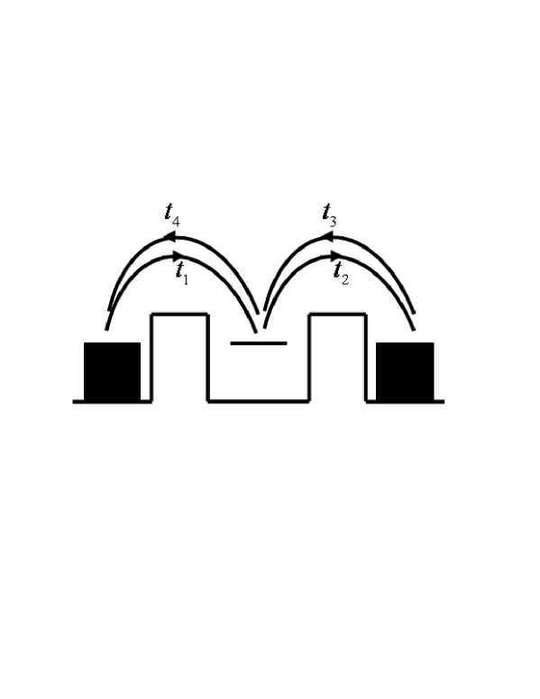
Figure 9: The tunneling scenario of an adiabatic quantum pump. The two shadowed blocks represent the left and right electron reservoirs respectively. The two barriers oscillate adiabatically in time. The middle bar indicates the single-particle state between the two barriers. The Fermi levels of the two reservoirs are the same and are leveled to the single-particle state within the conductor. $t_{1}$-$t_{4}$ indicate the transmission amplitudes between one of the two reservoirs and the middle single-particle state.

The mechanisms of an adiabatic quantum pump can be demonstrated in a mesoscopic system modulated by two oscillating barriers (see Fig. 9). To prominently picture the charge flow driven process within a cyclic period, the two potential barriers are modulated with a phase difference of $\pi/2$ in the manner of $U_{1}=U_{0}+U_{1\omega}\sin t$ and $U_{2}=U_{0}+U_{2\omega}\sin(t+\pi/2)$. Our discussion is within the framework of the single electron approximation and coherent tunneling. The Pauli principle is taken into account throughout the pumping process. The Fermi energy of the two reservoirs and the inner single-particle state energy are equalized to eliminate the external bias and secure energy-conserved tunneling [The kinetic properties (charge current, heat current, etc.) depend on the values of the scattering matrix within the energy interval of the order of ${\rm{max}}(k_{B}T,\hbar\omega)$ near the Fermi energy. In the low-frequency ($\omega\rightarrow 0$) and low-temperature ($T\rightarrow 0$) limit we assume the scattering matrix to be energy independent]. As shown in Fig. 9, the transmission strengths between one of the reservoirs and the inner single-particle state are denoted by $t_{1}$-$t_{4}$. When $t\in[0,\pi/2]$, $\sin t$ changes from 0 to 1 and $\sin(t+\pi/2)$ changes from 1 to 0. Considering the time-averaged effect, the chance of $U_{1}>U_{2}$ and $U_{1}<U_{2}$ is equal. Therefore, the probability of $t_{1}$ and $t_{3}$ balance out. The tunneling quantified by $t_{2}$ and $t_{4}$ do not occur since the inner particle state is not occupied. When $t\in[\pi/2,\pi]$, $\sin t$ changes from 1 to 0 and $\sin(t+\pi/2)$ changes from 0 to -1. $U_{1}>U_{2}$ invariably holds in this time regime. The probability of $t_{3}$ prevails and a net particle flow is driven from the right reservoir to the middle state. When $t\in[\pi,3\pi/2]$, $\sin t$ changes from 0 to -1 and $\sin(t+\pi/2)$ changes from -1 to 0. The probability of $t_{2}$ and $t_{4}$ balance out and the tunneling quantified by $t_{1}$ and $t_{3}$ are excluded from the Pauli principle. No net time-averaged tunneling occurs. When $t\in[3\pi/2,2\pi]$, $\sin t$ changes from -1 to 0 and $\sin(t+\pi/2)$ changes from 0 to 1. $U_{1}$ maintains a lower height than $U_{2}$, which drives the particle in the inner state to the left reservoir. Through one whole pumping cycle, electrons are pumped from the right reservoir to the left by absorbing energy from the two oscillating sources. The tunneling is governed by quantum coherence. In each period, the pumping process repeats and the particles are driven continuously in the same direction as time accumulates. Direction-reversed pumped current can be obtained with reversed phase difference of the two oscillating gates. The direction of the pumped current is from the phase-leading gate to the phase-lagged one without exception when we assume that higher barriers admit smaller transmission probability. It can find resemblance in its classical turnstile counterpartRef61 in which the fore-opened gate admits transmission ahead of the later-opened one driving currents in corresponding manner.

The current and noise properties in various quantum pump structures and devices were investigated such as the magnetic-barrier-modulated two dimensional electron gasRef4 , mesoscopic one-dimensional wireRef6 ; Ref65 , quantum-dot structuresRef61 ; Ref5 ; Ref11 ; Ref12 ; Ref71 , mesoscopic rings with Aharonov-Casher and Aharonov-Bohm effectRef7 , magnetic tunnel junctionsRef10 , chains of tunnel-coupled metallic islandsRef68 , the nanoscale helical wireRef69 ,the Tomonaga-Luttinger liquidRef67 , and garphene-based devicesRef63 ; Ref64 . Theory also predicts that charge can be pumped by oscillating one parameter in particular quantum configurationsRef66 . A recent experimentRef70 based on two parallel quantized charge pumps offers a way forward to the potential application of quantum pumping in quantum information processing, the generation of single photons in pairs and bunches, neural networking, and the development of a quantum standard for electrical current. Correspondingly, theoretical techniques have been put forward for the treatment of the quantum pumpsRef2 ; Ref3 ; Ref18 ; Ref65 ; Ref68 ; Ref72 . One of the most prominent is the scattering approach proposed by Brouwer who presented a formula that relates the pumped current to the parametric derivatives of the scattering matrix of the system. Driven by adiabatic and weak modulation (the ac driving amplitude is small compared to the static potential), the pumped current was found to vary in a sinusoidal manner as a function of the phase difference between the two oscillating potentials. It increases linearly with the frequency in line with experimental finding. The Floquet scattering theory is developedRef72 for quantum-mechanical pumping in mesoscopic conductors. It can be used to investigate quantum pumping behavior at arbitrary pumping amplitude and frequency.

As an example to demonstrate the Floquet scattering theory, we focus on the experimentally observed deviation from the weak-pumping theory with only the first-order parametric derivative of the scattering matrix considered. By expanding the scattering matrix to higher orders of the time and modulation amplitude, experimental observation can be interpreted by multi-energy-quantum-related processes.

III.2 Theoretical formulation

We use the scattering matrix approach to describe the response of a mesoscopic phase-coherent sample to two slowly oscillating (with a frequency $\omega$) external real parameters $X_{j}(t)$ (gate potential, magnetic flux, etc.),

$$\begin{array}[]{*{20}c}{X_{j}\left(t\right)=X_{0,j}+X_{\omega,j}e^{i\left({\omega t-\varphi_{j}}\right)}+X_{\omega,j}e^{-i\left({\omega t-\varphi_{j}}\right)},}&{j=1,2.}\\ \end{array}$$ (31)

$X_{0,j}$ and $X_{\omega,j}$ measure the static magnitude and ac driving amplitude of the two parameters, respectively. The phase difference between the two drivers is defined as $\phi=\varphi_{1}-\varphi_{2}$. The mesoscopic conductor is connected to two reservoirs at zero bias. The scattering matrix $\hat{s}$ being a function of parameters $X_{j}(t)$ depends on time.

A time-dependent scattering matrix can be introduced as follows.

$$\hat{b}_{\alpha}\left(t\right)=\int_{-\infty}^{\infty}{S_{\alpha\beta}\left({t,t^{\prime}}\right)\hat{a}_{\beta}\left({t^{\prime}}\right)dt^{\prime}},\begin{array}[]{*{20}c}{}\hfil&{t\geq t^{\prime}.}\\ \end{array}$$ (32)

Its Wigner transform reads

$$S_{\alpha\beta}\left({E,t}\right)=\int_{-\infty}^{\infty}{e^{iE\left({t-t^{\prime}}\right)}S_{\alpha\beta}\left({t,t^{\prime}}\right)dt^{\prime}}.$$ (33)

We assume the scattering time $t-t^{\prime}$ is small. Up to corrections of order $\hbar\omega/\gamma$ ($\gamma$ measures the escape rate), the matrix $S_{\alpha\beta}\left({E,t}\right)$ is equal to the “instantaneous” scattering matrix $S_{X}(E)$, which is obtained by “freezing” all parameters $X_{j}$ to their values at time $t$. Below, we use the instant scattering matrix $\hat{s}\left(t\right)$ in place of $S_{\alpha\beta}\left({E,t}\right)$ to describe the physics for simplicity. The kinetic properties (charge current, heat current, etc.) depend on the values of the scattering matrix within the energy interval of the order of ${\rm{max}}(k_{B}T,\hbar\omega)$ near the Fermi energy. In the low-frequency ($\omega\rightarrow 0$) and low-temperature ($T\rightarrow 0$) limit we assume the scattering matrix to be energy independent. To investigate the deviation from the small amplitude $X_{\omega,j}$ limit, we expand the scattering matrix $\hat{s}(t)$ into Taylor series of $X_{j}(t)$ to second order at $X_{0,j}$ with the terms linear and quadratic of $X_{\omega,j}$ present in the expansion,

$$\hat{s}\left(t\right)\approx\hat{s}_{0}\left({X_{0,j}}\right)+\hat{s}_{-\omega}e^{i\omega t}+\hat{s}_{+\omega}e^{-i\omega t}+\hat{s}_{2}+\hat{s}_{-2\omega}e^{2i\omega t}+\hat{s}_{+2\omega}e^{-2i\omega t},$$ (34)

with

$$\left\{\begin{array}[]{l}\hat{s}_{\pm\omega}=\sum\limits_{j=1,2}{X_{\omega,j}e^{\pm i\varphi_{j}}{{\partial\hat{s}}\mathord{\left/{\vphantom{{\partial\hat{s}}{\partial X_{j}}}}\right.\kern-1.2pt}{\partial X_{j}}}},\\ \hat{s}_{2}=\sum\limits_{j=1,2}{X_{\omega,j}^{2}{{\partial^{2}\hat{s}}\mathord{\left/{\vphantom{{\partial^{2}\hat{s}}{\partial X_{j}^{2}}}}\right.\kern-1.2pt}{\partial X_{j}^{2}}}},\\ \hat{s}_{\pm 2\omega}=\frac{1}{2}\sum\limits_{j=1,2}{X_{\omega,j}^{2}e^{\pm 2i\varphi_{j}}{{\partial^{2}\hat{s}}\mathord{\left/{\vphantom{{\partial^{2}\hat{s}}{\partial X_{j}^{2}}}}\right.\kern-1.2pt}{\partial X_{j}^{2}}}}.\\ \end{array}\right.$$ (35)

It can be seen from the equations that higher orders of the Fourier spectra enter into the scattering matrix. As a result, both the nearest and next nearest sidebands are taken into account, which implies that a scattered electron can absorb or emit an energy quantum of $\hbar\omega$ or $2\hbar\omega$ before it leaves the scattering region. In principle, third or higher orders in the Taylor series can be obtained accordingly. However, the higher-order parametric derivatives of the scatter matrix diminish dramatically and approximate zero. Numerical calculation demonstrates that even in relatively large amplitude modulation, their contribution is negligible.

The pumped current depends on the values of the scattering matrix within the energy interval of the order of $\max\left({k_{B}T,2\hbar\omega}\right)$ near the Fermi energy. In the low-temperature limit ($T\to 0$), an energy interval of $2\hbar\omega$ is opened during the scattering process.

The mesoscopic scatterer is coupled to two reservoirs with the same temperatures $T$ and electrochemical potentials $\mu$. Electrons with the energy $E$ entering the scatterer are described by the Fermi distribution function $f_{0}(E)$, which approximates a step function at a low temperature. Due to the interaction with an oscillating scatterer, an electron can absorb or emit energy quanta that changes the distribution function. A single transverse channel in one of the leads is considered. Applying the hypothesis of an instant scattering, the scattering matrix connecting the incoming and outgoing states can be written as

$$\hat{b}_{\alpha}\left(t\right)=\sum\limits_{\beta}{s_{\alpha\beta}\left(t\right)\hat{a}_{\beta}\left(t\right)}.$$ (36)

Here $s_{\alpha\beta}$ is an element of the scattering matrix $\hat{s}$; the time-dependent operator is $\hat{a}_{\alpha}\left(t\right)=\int{dE\hat{a}_{\alpha}\left(E\right)e^{{{-iEt}\mathord{\left/{\vphantom{{-iEt}\hbar}}\right.\kern-1.2pt}\hbar}}}$, and the energy-dependent operator ${\hat{a}_{\alpha}\left(E\right)}$ annihilates particles with total energy E incident from the $\alpha$ lead into the scatter and obey the following anticommutation relations

$$\left[{\hat{a}_{\alpha}^{\dagger}\left(E\right),\hat{a}_{\beta}\left({E^{\prime}}\right)}\right]=\delta_{\alpha\beta}\delta\left({E-E^{\prime}}\right).$$ (37)

Note that above expressions correspond to single- (transverse) channel leads and spinless electrons. For the case of many-channel leads each lead index ($\alpha$, $\beta$, etc.) includes a transverse channel index and any repeating lead index implies implicitly a summation over all the transverse channels in the lead. Similarly an electron spin can be taken into account.

Using Eqs. (34) and (36) and after a Fourier transformation we obtain

$$\begin{array}[]{l}\hat{b}_{\alpha}\left(E\right)=\sum\limits_{\beta}{\left[{\hat{s}_{0,\alpha\beta}\hat{a}_{\beta}\left(E\right)+\hat{s}_{2,\alpha\beta}\hat{a}_{\beta}\left(E\right)+\hat{s}_{-\omega,\alpha\beta}\hat{a}_{\beta}\left({E+\hbar\omega}\right)}\right.}\\ \left.{+\hat{s}_{+\omega,\alpha\beta}\hat{a}_{\beta}\left({E-\hbar\omega}\right)+\hat{s}_{-2\omega,\alpha\beta}\hat{a}_{\beta}\left({E+2\hbar\omega}\right)+\hat{s}_{+2\omega,\alpha\beta}\hat{a}_{\beta}\left({E-2\hbar\omega}\right)}\right].\\ \end{array}$$ (38)

The distribution function for electrons leaving the scatterer through the lead $\alpha$ is $f_{\alpha}^{\left({out}\right)}\left(E\right)=\left\langle{\hat{b}_{\alpha}^{\dagger}\left(E\right)\hat{b}_{\alpha}\left(E\right)}\right\rangle$, where $\left\langle\cdots\right\rangle$ means quantum-mechanical averaging. Substituting Eq. (38) we find

$$\begin{array}[]{l}f_{\alpha}^{\left({out}\right)}\left(E\right)=\sum\limits_{\beta}{\left[{\left|{\hat{s}_{0,\alpha\beta}+\hat{s}_{2,\alpha\beta}}\right|^{2}f_{0}\left(E\right)+\left|{\hat{s}_{-\omega,\alpha\beta}}\right|^{2}f_{0}\left({E+\hbar\omega}\right)}\right.}\\ \left.{\left|{\hat{s}_{+\omega,\alpha\beta}}\right|^{2}f_{0}\left({E-\hbar\omega}\right)+\left|{\hat{s}_{-2\omega,\alpha\beta}}\right|^{2}f_{0}\left({E+2\hbar\omega}\right)+\left|{\hat{s}_{+2\omega,\alpha\beta}}\right|^{2}f_{0}\left({E-2\hbar\omega}\right)}\right].\\ \end{array}$$ (39)

The distribution function for outgoing carriers is a nonequilibrium distribution function generated by the nonstationary scatterer. The Fourier amplitudes of the scattering matrix ${\left|{\hat{s}_{-\omega,\alpha\beta}}\right|^{2}}$ (${\left|{\hat{s}_{+\omega,\alpha\beta}}\right|^{2}}$) is the probability for an electron entering the scatterer through the lead $\beta$ and leaving the scatterer through the lead $\alpha$ to emit (to absorb) an energy quantum $\hbar\omega$ and ${\left|{\hat{s}_{-2\omega,\alpha\beta}}\right|^{2}}$ (${\left|{\hat{s}_{+2\omega,\alpha\beta}}\right|^{2}}$) is that of the energy quantum $2\hbar\omega$ process. ${\left|{\hat{s}_{0,\alpha\beta}+\hat{s}_{2,\alpha\beta}}\right|^{2}}$ is the probability for the same scattering without the change of an energy with the second-order term $\hat{s}_{2,\alpha\beta}$ much smaller than the zero-order term $\hat{s}_{0,\alpha\beta}$ in weak-modulation limit ($X_{\omega,j}\ll X_{0,j}$) and can be omitted therein.

Using the distribution functions $f_{0}(E)$ for incoming electrons and $f_{\alpha}^{out}(E)$ for outgoing electrons, the pumped current measured at lead $\alpha$ reads

$$I_{p}=\frac{e}{{2\pi\hbar}}\int_{0}^{\infty}{\left\langle{\hat{b}_{\alpha}^{\dagger}\left(E\right)\hat{b}_{\alpha}\left(E\right)}\right\rangle-\left\langle{\hat{a}_{\alpha}^{\dagger}\left(E\right)\hat{a}_{\alpha}\left(E\right)}\right\rangle dE}.$$ (40)

Substituting Eqs. (34) and (30) we get

$$\begin{array}[]{c}I_{p}=\frac{{e\omega}}{{2\pi}}\sum\limits_{\beta,j_{1},j_{2}}{X_{\omega,j_{1}}X_{\omega,j_{2}}\frac{{\partial s_{\alpha\beta}}}{{\partial X_{j_{1}}}}\frac{{\partial s_{\alpha\beta}^{*}}}{{\partial X_{j_{2}}}}2i\sin\left({\varphi_{j_{1}}-\varphi_{j_{2}}}\right)}\\ +\frac{{e\omega}}{{2\pi}}\sum\limits_{\beta,j_{1},j_{2}}{X_{\omega,j_{1}}^{2}X_{\omega,j_{2}}^{2}\frac{{\partial^{2}s_{\alpha\beta}}}{{\partial X_{j_{1}}^{2}}}\frac{{\partial^{2}s_{\alpha\beta}^{*}}}{{\partial X_{j_{2}}^{2}}}i\sin\left[{2\left({\varphi_{j_{1}}-\varphi_{j_{2}}}\right)}\right]}.\\ \end{array}$$ (41)

Quantum pumping properties beyond the theory based on first-order parametric derivative of the scattering matrix are demonstrated in Eq. (41). By taking higher orders of the Fourier spectrum of the scattering matrix into consideration, double $\hbar\omega$ energy quantum (or a $2\hbar\omega$ energy quantum) emission (absorption) processes coact with single $\hbar\omega$ quantum processes. In the weak-modulation limit, the second term in the right-hand side of Eq. (41) is small, which implies that double $\hbar\omega$ quantum processes are weak and therefore not observable. As the ac driving amplitude is enlarged, this term increases markedly and contribution from double $\hbar\omega$ quantum processes takes effect. As a result, the dependence of the pumped current on the phase difference between two driving oscillations deviates from sinusoidal and changes from $\sin\phi$ to $\sin 2\phi$, which is observed in experimentRef1 . Moreover, the relation between the pumped current and the ac driving amplitude $X_{\omega,j}$ is reshaped. It is also seen that the linear dependence of the pumped current on the oscillation frequency holds for multi-quanta-related processes.

III.3 Numerical results and interpretations

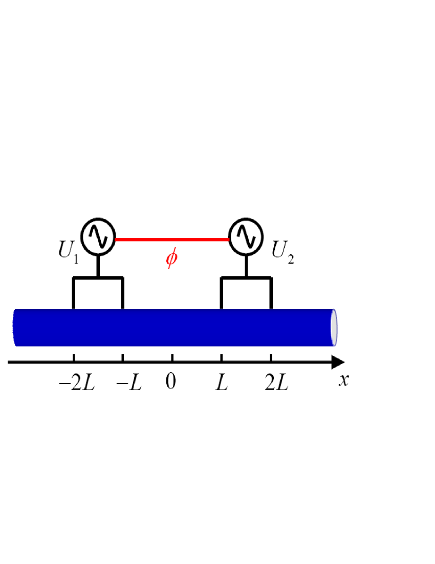
Figure 10: Schematics of the quantum pump: a nanowire modulated by two ac driven potential barriers.

Here, numerical results of the pumped current in a two-oscillating-potential-barrier modulated nanowire are presented and comparison with experiment is given. We consider a nanowire modulated by two gate potential barriers with equal width $L=20$ Å separated by a $2L=40$ Å width well (see Fig. 10). The electrochemical potential of the two reservoirs $\mu$ is set to be $60$ meV according to the resonant level within the double-barrier structure. The two oscillating parameters in Eq. (31) correspond to the two ac driven potential gates $X_{1,2}\left(t\right)\to U_{1,2}\left(t\right)$ with all the other notations correspond accordingly. We set the static magnitude of the two gate potentials $U_{0,1}=U_{0,2}=U_{0}=100$ meV and the ac driving amplitude of the modulations equal $U_{\omega,1}=U_{\omega,2}=U_{\omega}$.

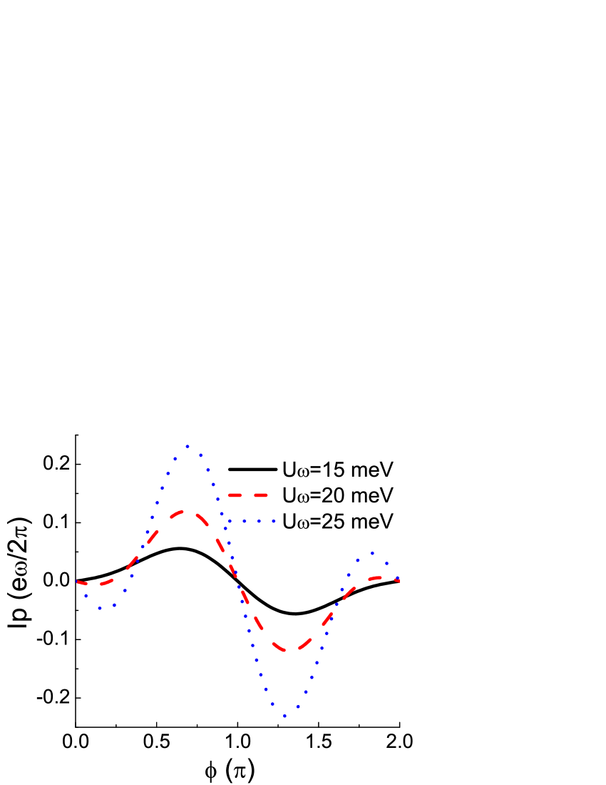
Figure 11: Pumped current as a function of the phase difference between the two modulations for different ac driving amplitudes.

In Fig. 11, the dependence of the pumped current on the phase difference between the two ac oscillations is presented. In weak-modulation regime (namely $U_{\omega}$ is small), sinusoidal behavior dominates. Here, three relatively large $U_{\omega}$ is selected to reveal the deviation from the sinusoidal dependence. (The magnitude of the pumped current mounts up in power-law relation as a function of $U_{\omega}$ as shown in Fig. 12. The sinusoidal curve for small $U_{\omega}$ would be flat and invisible in the same coordinate range.) It can be seen from the figure that the $I_{p}$-$\phi$ relation varies from sinusoidal ($\sin\phi$) to double-sinusoidal ($\sin 2\phi$) as the ac oscillation amplitude is increased. The interpretation follows from Eq. (41). The single $\hbar\omega$ quantum emission (absortion) processes feature a sinusoidal behavior while the $2\hbar\omega$ quantum emission (absortion) processes feature a double-sinusoidal behavior when the Fourier index is doubled. As $U_{\omega}$ is increased, double $\hbar\omega$ quantum processes gradually parallel and outweigh the single $\hbar\omega$ quantum ones. It is also demonstrated that when the single $\hbar\omega$ quantum processes have the effect of $\sin\phi$ dependence, the double $\hbar\omega$ quantum processes induce a $-\sin 2\phi$ contribution with a sign flip, which can be understood from the sign change of the derivative of the scattering matrix. The effect of three- and higher $\hbar\omega$ quantum processes is small even for large $U_{\omega}$ comparable to $U_{0}$. The experimental observationsRef1 as a deviation from the weak-modulation limit are revealed by our theory.

ExperimentRef1 also discovered that for weak pumping the dependence of the pumped current on the pumping strength obeys a power of 2 relation, as expected from the simple loop-area argumentRef2 ; for strong pumping, power of 1 and 1/2 relation is observed. We presented in Fig. 12 the numerical results based on our theory of the $I_{p}$-$U_{\omega}$ relation at a fixed $\phi$. To demonstrate its power-law dependence, natural logarithm of the variables is applied. From Eq. (41), it can be seen that for large ac driving amplitude $U_{\omega}$, contribution of double $\hbar\omega$ quantum processes (formulated in the second term on the right hand side of the equation) causes the $I_{p}$-$U_{\omega}$ relation to deviate from its weak-modulation limit, the latter of which is $I_{p}\propto U_{\omega}^{2}$. For different phase difference between the two ac drivers, the deviation is different. At $\phi=\pi$ the pumped current is invariably zero regardless of the order of approximation determined by time-reversal symmetry. At $\phi=\pi/2$, $\sin 2\phi$ is exact zero, and no difference is incurred by introducing higher order effect. If we shift the value of $\phi$ to $0.49\pi$, the abating effect of the double $\hbar\omega$ quantum processes has the order of $U_{\omega}^{4}$ with the small second-order parametric derivative of the scattering matrix smoothing that effect a bit. Consequently, a power of $2\to 1\to 1/2$ relation is obtained and visualized by the curve fit, which is analogous to experimental findings. For different values of $\phi$, sharper abating and augmental effect occurs with analogous mechanisms. It is possible that the experimentRef1 was done at the phase difference close to $\pi/2$ while trying to approach maximal pumped current in the adiabatic and weak-pumping limit.

IV Summary and future directions

The scattering matrix method is initiated by Landauer and Büttiker to investigate the conductance of multi-terminal and multi-channel mesoscopic conductors. The spin degree of freedom can be included in the formalism by enlargement of the dimension of the scattering matrix. The current-current correlation and spin-spin correlation, such as the shot noise, can be calculated from the cross products of the scattering matrix. Along this direction, higher-order correlation function can also be considered. Dynamic transport processes including the quantum pumping behavior can be dealt with by the time-dependent scattering approach.

The development of the scattering theory enables its potential applications in currently open issues. The interaction can be included to the scattering matrix by the renormalization factors. The shot noise properties in various conductors with active spin degree of freedom can be considered. The time-dependent scattering theory provides a way to deal with dynamic quantum issues. Some particular problems include non-harmonically driven quantum pumping, spin pumping in racetrack memory applications, and multiferroic transport dynamics, etc..

V Acknowledgements

This project was supported by the Nature Science Foundation of SCUT (No. x2lxE5090410) and the Graduate Course Construction Project of SCUT (No. yjzk2009001). The author would like to express sincere appreciation to Professor Wenji Deng, Dr. Brian M. Walsh, Professor Jamal Berakdar, Professor Michael Moskalets, and Professor Liliana Arrachea for valuable enlightenment to the topic from discussions with them.

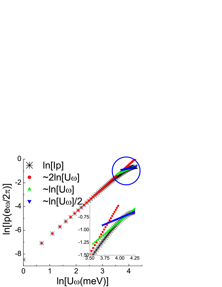
Figure 12: Pumped current as a function of the ac driving amplitude $U_{\omega}$ along with fits to $I_{p}\propto U_{\omega}^{2}$ (red solid circle) below 35 meV, $I_{p}\propto U_{\omega}$ (green upward triangle) below 41 meV, and $I_{p}\propto U_{\omega}^{1/2}$ above 41 meV (blue downward triangle). To demonstrate its power-law dependence, natural logarithm of the variables is applied. The phase difference between the two ac driver $\phi=0.49\pi$. Inset is the zoom-in of the circled region.

References

- (1) D. K. Ferry and S. M. Goodnick, in Transport in Nanostructures, (Cambridge University Press, 1997).
- (2) R. Landauer, IBM J. Res. Develop. 1, 223 (1957); R. Landauer, Phil. Mag. 21, 863 (1970); R. Büttiker, Y. Imry, R. Landauer, and S. Pinhas, Phys. Rev. B 31, 6207 (1985).
- (3) I. Lo, W. C. Mitchel, R. E. Perrin, R. L. Messham, and M. Y. Yen, Phys. Rev. B 43, 11787 (1991).
- (4) M. L. Polianski, M. G. Vavilov, and P. W. Brouwer, Phys. Rev. B 65, 245314 (2002).
- (5) Y. M. Blanter and M. Büttiker, Physics Reports 336, 1 (2000).
- (6) V. V. Kuznetsov, E. E. Mendez, J. D. Bruno, and J. T. Pham, Phys. Rev. B 58, R10159 (1998).
- (7) Y. P. Li, A. Zaslavsky, D. C. Tsui, M. Santos, and M. Shayegan, Phys. Rev. B 41, 8388 (1990).
- (8) G. Iannaccone, G. Lombardi, M. Macucci, and B. Pellegrini, Phys. Rev. Lett. 80, 1054 (1998).
- (9) N. V. Alkeev, V. E. Lyubchenko, C. N. Ironside, J. M. L. Figueiredo, and C.R. Stanley, J. Commun. Technol. Electron. 47, 228 (2002).
- (10) N. V. Alkeev, V. E. Lyubchenko, C. N. Ironside, S. G. McMeekin, and A. M. P. Leite, J. Commun. Technol. Electron. 45, 911 (2000).
- (11) J. H. Davies, P. Hyldgaard, S. Hershfield, and J. W. Wilkins, Phys. Rev. B 46, 9620 (1992).
- (12) L. Y. Chen and C. S. Ting, Phys. Rev. B 43, 4534 (1991).
- (13) V. Y. Aleshkin, L. Reggiani, and M. Rosini, Phys. Rev. B 73, 165320 (2006).
- (14) R. Zhu and Y. Guo, J. Appl. Phys. 102, 083706 (2007).
- (15) Y. Guo, L. Han, R. Zhu, and W. Xu, Eur. Phys. J. B 62, 45 (2008).
- (16) R. Zhu and Y. Guo, J. Appl. Phys. 103, 073717 (2008).
- (17) R. Zhu and Y. Guo, Appl. Phys. Lett. 91, 252113 (2007).
- (18) R. Zhu and Y. Guo, Appl. Phys. Lett. 90, 232104 (2007).
- (19) G. Iannaccone, M. Macucci, and B. Pellegrini, Phys. Rev. B 55, 4539 (1997).
- (20) A. Voskoboynikov, S.S. Lin, C.P. Lee, and O. Tretyak, J. Appl. Phys. 87, 387 (2000).
- (21) T. Koga, J. Nitta, H. Takayanagi, and S. Datta, Phys. Rev. Lett. 88, 126601 (2002).
- (22) D.Z.-Y. Ting and X. Cartoixà, Appl. Phys. Lett. 81, 4198 (2002).
- (23) D.Z.-Y. Ting and X. Cartoixà, Appl. Phys. Lett. 83, 1391 (2003).
- (24) M. Yang and S.-S. Li, Phys. Rev. B 72, 193310 (2005).
- (25) V.I. Perel’, S.A. Tarasenko, I.N. Yassievich, S.D. Ganichev, V.V. Bel’kov, and W. Prettl, Phys. Rev. B 67, 201304(R) (2003).
- (26) E.L. Ivchenko and G.E. Pikus, Superlattices and Other Heterostructures. Symmetry and Optical Phenomena (Springer, Berlin, 1995) [2nd ed., 1997].
- (27) G. Dresselhaus, Phys. Rev. 100, 580 (1955).
- (28) A.E. Botha and M.R. Singh, Phys. Rev. B 67, 195334 (2003).
- (29) W. Li and Y. Guo, Phys. Rev. B 73, 205311 (2006).
- (30) M.M. Glazov, P.S. Alekseev, M.A. Odnoblyudov, V.M. Chistyakov, S.A. Tarasenko, and I.N. Yassievich, Phys. Rev. B 71, 155313 (2005).
- (31) J.H. Davies, The physics of low-dimensional semiconductors (Cambridge University Press, Cambridge, 1998).
- (32) M. Büttiker, Phys. Rev. B 46, 12485 (1992).
- (33) In the positive differential conductance (PDC) region, results for the case considering charging effect or Coulomb interaction are close to those neglecting Coulomb effect in both coherent and sequential approaches (see Refs. Ref36, and Ref60, ), i.e., the effect of Coulomb interaction on shot noise is weak in the region. Thus it is reasonable to neglect it in the PDC region.
- (34) L. P. Kouwenhoven, A. T. Johnson, N. C. van der Vaart, C. J. P. M. Harmans, and C. T. Foxon, Phys. Rev. Lett. 67, 1626 (1991).
- (35) D. J. Thouless, Phys. Rev. B 27, 6083 (1983).
- (36) M. Switkes, C. M. Marcus, K. Campman, and A. C. Gossard, Science 283, 1905 (1999).
- (37) P. W. Brouwer, Phys. Rev. B 58, R10135 (1998). M. Büttiker, H. Thomas, and A. Prêtre, Z. Phys. B 94, 133 (1994); Phys. Rev. Lett. 70, 4114 (1993).
- (38) M. Moskalets and M. Büttiker, Phys. Rev. B 66, 035306 (2002).
- (39) R. Benjamin and C. Benjamin, Phys. Rev. B 69, 085318 (2004).
- (40) H. C. Park and K. H. Ahn, Phys. Rev. Lett. 101, 116804 (2008).
- (41) P. Devillard, V. Gasparian, and T. Martin, Phys. Rev. B 78, 085130 (2008).
- (42) R. Citro and F. Romeo, Phys. Rev. B 73, 233304 (2006).
- (43) M. Moskalets and M. Büttiker, Phys. Rev. B 72, 035324 (2005).
- (44) M. Moskalets and M. Büttiker, Phys. Rev. B 75, 035315 (2007).
- (45) F. Romeoa and R. Citro, Eur. Phys. J. B 50, 483 (2006).
- (46) J. Splettstoesser, M. Governale and J. König, Phys. Rev. B 77, 195320 (2008).
- (47) M. Strass, P. Hänggi, and S. Kohler, Phys. Rev. Lett. 95, 130601 (2005).
- (48) J. E. Avron, A. Elgart, G. M. Graf, and L. Sadun, Phys. Rev. Lett. 87, 236601 (2001).
- (49) B. G. Wang, J. Wang, and H. Guo, Phys. Rev. B 65, 073306 (2002).
- (50) B. G. Wang and J. Wang, Phys. Rev. B. 66, 125310 (2002).
- (51) B. G. Wang, J. Wang, and H. Guo, Phys. Rev. B 68, 155326 (2003).
- (52) L. Arrachea, Phys. Rev. B 72, 125349 (2005).
- (53) Y. Tserkovnyak, A. Brataas, G. E. W. Bauer, and B. I. Halperin, Rev. Mod. Phys. 77, 1375 (2005).
- (54) D. C. Ralph and M. D. Stiles, J. Magn. Magn. Mater. 320, 1190 (2008).
- (55) R. Zhu and H. Chen, Appl. Phys. Lett. 95, 122111 (2009).
- (56) E. Prada, P. San-Jose, and H. Schomerus, Arxiv:0907.1568v1 (unpublished).
- (57) A. Agarwal and D. Sen, J. Phys.: Condens. Matter 19, 046205 (2007).
- (58) L. E. F. Foa Torres, Phys. Rev. B 72, 245339 (2005).
- (59) A. Agarwal and D. Sen, Phys. Rev. B 76, 235316 (2007).
- (60) N. Winkler, M. Governale, and J. König, Phys. Rev. B 79, 235309 (2009).
- (61) X. L. Qi and S. C. Zhang, Phys. Rev. B 79, 235442 (2009).
- (62) S. J. Wright, M. D. Blumenthal, M. Pepper, D. Anderson, G. A. C. Jones, C. A. Nicoll, and D. A. Ritchie, Phys. Rev. B 80, 113303 (2009).
- (63) F. Romeo and R. Citro, Phys. Rev. B 80, 165311 (2009).
- (64) M. Moskalets and M. Büttiker, Phys. Rev. B 66, 205320 (2002).