Approaching Throughput-optimality in Distributed CSMA Scheduling Algorithms with Collisions

Libin Jiang and Jean Walrand
EECS Department, University of California at Berkeley
{ljiang,wlr}@eecs.berkeley.edu
This work is supported by MURI grant BAA 07-036.18. Some main results of this paper appeared in [29].This is the longer version of a same-titled paper to appear in IEEE/ACM Transactions on Networking.
Abstract

It was shown recently that CSMA (Carrier Sense Multiple Access)-like distributed algorithms can achieve the maximal throughput in wireless networks (and task processing networks) under certain assumptions. One important, but idealized assumption is that the sensing time is negligible, so that there is no collision. In this paper, we study more practical CSMA-based scheduling algorithms with collisions. First, we provide a Markov chain model and give an explicit throughput formula which takes into account the cost of collisions and overhead. The formula has a simple form since the Markov chain is “almost” time-reversible. Second, we propose transmission-length control algorithms to approach throughput optimality in this case. Sufficient conditions are given to ensure the convergence and stability of the proposed algorithms. Finally, we characterize the relationship between the CSMA parameters (such as the maximum packet lengths) and the achievable capacity region.

Index Terms:
Distributed scheduling, CSMA, Markov chain, convex optimization

I Introduction

Efficient resource allocation is essential to achieve high utilization of a class of networks with resource-sharing constraints, such as wireless networks and stochastic processing networks (SPN [5]). In wireless networks, certain links cannot transmit at the same time due to the interference constraints among them. In a SPN, two tasks cannot be processed simultaneously if they both require monopolizing a common resource. A scheduling algorithm determines which link to activate (or which task to process) at a given time without violating these constraints. Designing efficient distributed scheduling algorithms to achieve high throughput is especially a challenging task [4].

Maximal-weight scheduling (MWS) [3] is a classical throughput-optimal algorithm. That is, MWS can stabilize all queues in the network as long as the arrival rates are within the capacity region. MWS operates in slotted time. In each slot, a set of non-conflicting links (called an “independent set”, or “IS”) that have the maximal weight (i.e., summation of queue lengths) are scheduled. However, implementing MWS in general networks is quite difficult for two reasons. (i) MWS is inherently a centralized algorithm and is not amenable to distributed implementation; (ii) finding a maximal-weighted IS (in each slot) is NP-complete in general and is hard even for centralized algorithms.

On the other hand, there has been active research on low-complexity but suboptimal scheduling algorithms. For example, reference [6] shows that Maximal Scheduling can only guarantee a fraction of the network capacity. A related algorithm has been studied in [7] in the context of IEEE 802.11 networks. Longest-Queue-First (LQF) algorithm (see, for example, [9, 10, 11, 12]), which greedily schedules queues in the descending order of the queue lengths, tends to achieve higher throughput than Maximal Scheduling, although it is not throughput-optimal in general [10]. Reference [13] proposed random-access-based algorithms that can achieve performance comparable to that of maximal-size scheduling.

Recently, we proposed a distributed adaptive CSMA (Carrier Sense Multiple Access) algorithm [16] that is throughput-optimal for a general interference model, under certain assumptions (further explained later). The algorithm has a few desirable features. It is distributed (i.e., each node only uses its own backlog information), asynchronous (i.e., nodes do not need to synchronize their transmission) and requires no control message. (In [17], Rajagopalan and Shah independently proposed a similar randomized algorithm in the context of optical networks. Reference [18] showed that under a “node-exclusive” interference model, CSMA can be made throughput-optimal in an asymptotic regime.) We have also developed a joint algorithm in [16] that combined the adaptive CSMA scheduling with congestion control to approach the maximal total utility of competing data flows.

However, the algorithms in [16] assume an idealized CSMA protocol ([14, 25, 26, 27]), meaning that the sensing is instantaneous, so that conflicting links do not transmit at the same time (i.e., collisions do not occur). In many situations, however, this is an unnatural assumption. For example, in CSMA/CA wireless networks, due to the propagation delay and processing time, sensing is not instantaneous. Instead, time can be viewed as divided into discrete minislots, and collisions happen if multiple conflicting links try to transmit in the same minislot. When a collision occurs, all links that are involved lose their packets, and will try again later.

In this paper, we study this important practical issue when designing CSMA-based scheduling algorithms. We follow four main steps: (1) we first present a Markov chain model for a simple CSMA protocol with collisions, and give an explicit throughput formula (in section II) that has a simple form since the Markov chain is “almost” time-reversible; (2) we show that the algorithms in [16] can be extended to approach throughput optimality even with collisions (section III); (3) we give sufficient conditions to ensure the convergence/stability of the proposed algorithms (section III); (4) finally, we discuss the tradeoff between the achievable capacity region and short-term fairness, and we characterize the relationship between the CSMA parameters (such as the maximum packet lengths) and the achievable capacity region.

Although step (2) can be viewed as a generalization of [16], we believe that this generalization is important and non-trivial. The importance, as mentioned above, is because collisions are unavoidable in CSMA/CA wireless networks, and the collision-free model used in [16] does not provide enough accuracy. The generalization is non-trivial for the following reasons. Step (2) requires the result of step (1). In step (1), the Markov chain used to model the CSMA protocol is no longer time-reversible as in [16]. We need to re-define the state space in order to compute the service rates it can provide. Interestingly, as a result of our design the chain is “almost” time-reversible which can be exploited. In step (2), in view of the expression of service rates derived in step (1), it is important to realize that adjusting the backoff times as in [16] does not lead to the desirable throughput-optimal property. Instead, one should adjust the transmission lengths. Different from [16], we further show that the “optimal” CSMA parameters (in this case the mean transmission lengths) are unique. This fact is needed to establish the convergence of our algorithm in step (3).

We note that in a recent work [8], Ni and Srikant also proposed a CSMA-like algorithm to achieve near-optimal throughput with collisions taken into account. The algorithm in [8] uses synchronized and alternate control phase and data phase. It is designed to realize a discrete-time CSMA (in the data phase) which has the same stationary distribution as its continuous counterpart in [16]. The control phase does not contribute to the throughput and can be viewed as the protocol overhead. Different from [8], our algorithm here is asynchronous, and has more resemblance to the RTS/CTS mode in IEEE 802.11. Although the algorithm in [8] is quite elegant and could potentially be applied to other time-slotted systems, we believe that it is an interesting problem to understand how to use the asynchronous algorithm to achieve throughput-optimality. Also, due to its similarity to the RTS/CTS mode of IEEE 802.11, the throughput analysis in this paper could also deepen the understanding of 802.11 in general topologies.

II CSMA/CA-based scheduling with collisions

II-A Model

In this section we present a model for CSMA/CA-based scheduling with collisions. Note that the goal of the paper is not to propose a comprehensive model that captures all details for IEEE 802.11 networks and predict the performance of such networks (The literature in that area has been very rich. See, for example, [24, 25] and the references therein.) Instead, at a more abstract level, we are interested in a distributed scheduling algorithm that is inspired by CSMA/CA, and designing adaptive algorithms to approach throughput-optimality.

Consider a (single-channel) wireless network. Define a “link” as an (ordered) transmitter-receiver pair. Assume that there are K𝐾K links, and denote the set of links by 𝒩𝒩{\cal N} (then, K=|𝒩|𝐾𝒩K=|{\cal N}|). Without loss of generality, assume that each link has a capacity of 1. We say that two links conflict if they cannot transmit (or, “be active”) at the same time due to interference. (The conflict relationship is assumed to be symmetric.) Accordingly, define G𝐺G as the conflict graph. Each vertex in G𝐺G represents a link, and there is an edge between two vertexes if the corresponding links conflict. Note that this simple conflict model may not reflect all possible interference structures that could occur in wireless networks. However, it does provide a useful abstraction and has been used widely in literature (see, for example, [25] and [4]).

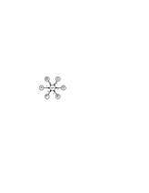
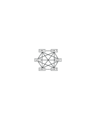
Fig. 1 (a) shows a wireless LAN with 6 links. The network’s conflict graph is a full graph (Fig. 1 (b)). (Circles represent nodes and rectangles represent links.) Fig. 2 (a) shows an ad-hoc network with 3 links. Assume that link 1, 2 conflict, and link 2, 3 conflict. Then the network’s conflict graph is Fig. 2 (b).
Refer to caption
(a) Network topology
Refer to caption
(b) Conflict graph
Figure 1: Infrastructure network
Refer to caption
(a) Network topology
Refer to caption
(b) Conflict graph
Figure 2: Ad-hoc network

Basic Protocol

We now describe the basic CSMA/CA protocol with fixed transmission probabilities (which suffices for our later development.) Let σ~~𝜎\tilde{\sigma} be the duration of each idle slot (or “minislot”). (σ~~𝜎\tilde{\sigma} should be at least the time needed by any wireless station to detect the transmission of any other station. Specifically, it accounts for the propagation delay, the time needed to switch from the receiving to the transmitting state, and the time to signal to the MAC layer the state of the channel [15]. The value of σ~~𝜎\tilde{\sigma} varies for different physical layers. In IEEE 802.11a, for example, σ~=9μs~𝜎9𝜇𝑠\tilde{\sigma}=9\mu s.) In the following we will simply use “slot” to refer to the minislot.

Assume that all links are saturated (i.e., always have packets to transmit). In each slot, if (the transmitter of) link i𝑖i is not already transmitting and if the medium is idle, the transmitter of link i𝑖i starts transmission with probability pisubscript𝑝𝑖p_{i}. If at a certain slot, link i𝑖i did not choose to transmit but a conflicting link starts transmitting, then link i𝑖i keeps silent until that transmission ends. If conflicting links start transmitting at the same slot, then a collision happens. [We assume that the network has no hidden node (HN). The case with HNs will be discussed in Section V-C. For possible ways to address the HN problem, please refer to [19] and its references.]

Each link transmits a short probe packet with length γ𝛾\gamma (similar to the RTS packet in 802.11) before the data is transmitted. (All “lengths” here are measured in number of slots and are assumed to be integers.) This increases the overhead of successful transmissions, but can avoid collisions of long data packets. When a collision happens, only the probe packets collide, so each collision lasts a length of γ𝛾\gamma. Assume that a successful transmission of link i𝑖i lasts τisubscript𝜏𝑖\tau_{i}, which includes a constant overhead τsuperscript𝜏\tau^{\prime} (composed of RTS, CTS, ACK, etc) and the data payload τipsuperscriptsubscript𝜏𝑖𝑝\tau_{i}^{p} which is a random variable. Clearly τiτsubscript𝜏𝑖superscript𝜏\tau_{i}\geq\tau^{\prime}. Let the p.m.f. (probability mass function) of τisubscript𝜏𝑖\tau_{i} be

Pr{τi=bi}=Pi(bi),bi𝒵++formulae-sequence𝑃𝑟subscript𝜏𝑖subscript𝑏𝑖subscript𝑃𝑖subscript𝑏𝑖for-allsubscript𝑏𝑖subscript𝒵absentPr\{\tau_{i}=b_{i}\}=P_{i}(b_{i}),\forall b_{i}\in{\cal Z}_{++} (1)

and assume that the p.m.f. has a finite support, i.e., Pi(bi)=0,bi>bmax>0formulae-sequencesubscript𝑃𝑖subscript𝑏𝑖0for-allsubscript𝑏𝑖subscript𝑏𝑚𝑎𝑥0P_{i}(b_{i})=0,\forall b_{i}>b_{max}>0.111The finite support assumption is not a restrictive one, since in practical wireless networks there is usually an upper bound on the packet size. However, the CSMA/CA Markov chain defined later is still ergodic even without the assumption. Then the mean of τisubscript𝜏𝑖\tau_{i} is

Ti:=E(τi)=b𝒵++bPi(b).assignsubscript𝑇𝑖𝐸subscript𝜏𝑖subscript𝑏subscript𝒵absent𝑏subscript𝑃𝑖𝑏T_{i}:=E(\tau_{i})=\sum_{b\in{\cal Z}_{++}}b\cdot P_{i}(b). (2)

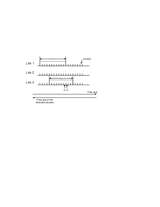
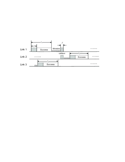
Fig. 3 illustrates the timeline of the 3-link network in Fig. 2 (b), where link 1 and 2 conflict, and link 2 and 3 conflict.

We note a subtle point in our modeling. In IEEE 802.11, a link can attempt to start a transmission only after it has sensed the medium as idle for a constant time (which is called DIFS, or “DCF Inter Frame Space”). To take this into account, DIFS is included in the packet transmission length τisubscript𝜏𝑖\tau_{i} and the collision length γ𝛾\gamma. In particular, for a successful transmission of link i𝑖i, DIFS is included in the constant overhead τsuperscript𝜏\tau^{\prime}. Although DIFS, as part of τsuperscript𝜏\tau^{\prime}, is actually after the payload, in Fig. 3 we plot τsuperscript𝜏\tau^{\prime} before the payload. This is for convenience and does not affect our results. So, under this model, a link can attempt to start a transmission immediately after the transmissions of its conflicting links end.

The above model is almost time-reversible such that a simple throughput formula can be derived. A process is “time-reversible” if the process and its time-reversed process are statistically indistinguishable [1]. Our model, in Fig. 3, reversed in time, follows the same protocol as described above, except for the order of the overhead and the payload, which are reversed. A key reason for this property is that the collisions start and finish at the same time. (This point will be made more precise in Appendix A.)
Refer to caption
Figure 3: Timeline in the basic model (In this figure, τi=Ti,i=1,2,3formulae-sequencesubscript𝜏𝑖subscript𝑇𝑖𝑖123\tau_{i}=T_{i},i=1,2,3 are constants.)

II-B Notation

Let the “on-off state” be x{0,1}K𝑥superscript01𝐾x\in\{0,1\}^{K} where xksubscript𝑥𝑘x_{k}, the k𝑘k-th element of x𝑥x, is such that xk=1subscript𝑥𝑘1x_{k}=1 if link k𝑘k is active (transmitting) in state x𝑥x, and xk=0subscript𝑥𝑘0x_{k}=0 otherwise. Thus, x𝑥x is a vector indicating which links are active in a given slot. Let G(x)𝐺𝑥G(x) be the subgraph of G𝐺G after removing all vertices (each representing a link) with state 0 (i.e., any link j𝑗j with xj=0subscript𝑥𝑗0x_{j}=0) and their associated edges. In general, G(x)𝐺𝑥G(x) is composed of a number of connected components (simply called “components”) Cm(x),m=1,2,,M(x)formulae-sequencesubscript𝐶𝑚𝑥𝑚12𝑀𝑥C_{m}(x),m=1,2,\dots,M(x) (where each component is a set of links, and M(x)𝑀𝑥M(x) is the total number of components in G(x)𝐺𝑥G(x)). If a component Cm(x)subscript𝐶𝑚𝑥C_{m}(x) has only one active link (i.e., |Cm(x)|=1subscript𝐶𝑚𝑥1|C_{m}(x)|=1), then this link is having a successful transmission; if |Cm(x)|>1subscript𝐶𝑚𝑥1|C_{m}(x)|>1, then all the links in the component are experiencing a collision. Let the set of “successful” links in state x𝑥x be S(x):={k|kCm(x) with |Cm(x)|=1}assign𝑆𝑥conditional-set𝑘𝑘subscript𝐶𝑚𝑥 with subscript𝐶𝑚𝑥1S(x):=\{k|k\in C_{m}(x)\text{ with }|C_{m}(x)|=1\}, and the set of links that are experiencing collisions be Z(x)𝑍𝑥Z(x). Also, define the “collision number” h(x)𝑥h(x) as the number of components in G(x)𝐺𝑥G(x) with size larger than 1. Fig. 4 shows an example. Note that the transmissions in a collision component Cm(x)subscript𝐶𝑚𝑥C_{m}(x) are “synchronized”, i.e., the links in Cm(x)subscript𝐶𝑚𝑥C_{m}(x) must have started transmitting in the same slot, and will end transmitting in the same slot after γ𝛾\gamma slots (the length of the probe packets).

Refer to caption
Figure 4: An example conflict graph (each square represents a link). In this on-off state x𝑥x, links 1, 2, 5 are active. So S(x)={5}𝑆𝑥5S(x)=\{5\}, Z(x)={1,2}𝑍𝑥12Z(x)=\{1,2\}, h(x)=1𝑥1h(x)=1.

II-C Computation of the service rates

In order to compute the service rates of all the links under the above CSMA protocol when all the links are saturated, we first define the underlying discrete-time Markov chain which we call the CSMA/CA Markov chain.

The Markov chain evolves slot by slot.222For the ease of analysis, we make the modeling assumption that the links are synchronized at the slot level. The state of the Markov chain in a slot is

w:={x,((bk,ak),k:xk=1)}w:=\{x,((b_{k},a_{k}),\forall k:x_{k}=1)\} (3)

where bksubscript𝑏𝑘b_{k} is the total length of the current packet link k𝑘k is transmitting, aksubscript𝑎𝑘a_{k} is the remaining time (including the current slot) before the transmission of link k𝑘k ends.

For example, in Fig. 5, the state w𝑤w and wsuperscript𝑤w^{\prime} are

Refer to caption
Figure 5: Example of the CSMA/CA Markov chain
w={x=(1,0,1)T,(b1=11,a1=1),(b3=10,a3=4)}𝑤𝑥superscript101𝑇formulae-sequencesubscript𝑏111subscript𝑎11formulae-sequencesubscript𝑏310subscript𝑎34w=\{x=(1,0,1)^{T},(b_{1}=11,a_{1}=1),(b_{3}=10,a_{3}=4)\} (4)

and

w={x=(0,0,1)T,(b3=10,a3=3)}.superscript𝑤𝑥superscript001𝑇formulae-sequencesuperscriptsubscript𝑏310superscriptsubscript𝑎33w^{\prime}=\{x=(0,0,1)^{T},(b_{3}^{\prime}=10,a_{3}^{\prime}=3)\}. (5)

Note that in any state w𝑤w as defined in (3), we have

(I) 1akbk,k:xk=11\leq a_{k}\leq b_{k},\forall k:x_{k}=1.

(II) Pk(bk)>0,kS(x)formulae-sequencesubscript𝑃𝑘subscript𝑏𝑘0for-all𝑘𝑆𝑥P_{k}(b_{k})>0,\forall k\in S(x).

(III) If kZ(x)𝑘𝑍𝑥k\in Z(x), then bk=γsubscript𝑏𝑘𝛾b_{k}=\gamma and ak{1,2,,γ}subscript𝑎𝑘12𝛾a_{k}\in\{1,2,\dots,\gamma\}. An important observation here is that the transmissions in a collision component Cm(x)subscript𝐶𝑚𝑥C_{m}(x) are “synchronized”, i.e., the links in Cm(x)subscript𝐶𝑚𝑥C_{m}(x) must have started transmitting at the same time, and will end transmitting at the same time, so all links in the component Cm(x)subscript𝐶𝑚𝑥C_{m}(x) have the same remaining time. (To see this, first note that in the case of a collision only the probe packets get transmitted, and their transmission times γ𝛾\gamma are identical for all links. Second, any two links i𝑖i and j𝑗j in this component with an edge between them must have started transmitting at the same time. Otherwise, if i𝑖i starts earlier, j𝑗j would not transmit since it already hears i𝑖i’s transmission; and vice versa. By induction, all links in the component must have started transmitting at the same time.) So, we can write ak=a(m)subscript𝑎𝑘superscript𝑎𝑚a_{k}=a^{(m)} for any kCm(x)𝑘subscript𝐶𝑚𝑥k\in C_{m}(x) where |Cm(x)|>1subscript𝐶𝑚𝑥1|C_{m}(x)|>1, and a(m)superscript𝑎𝑚a^{(m)} denotes the remaining time of the component Cm(x)subscript𝐶𝑚𝑥C_{m}(x).

We say that a state w𝑤w is valid iff it satisfies (I)~(III) above.

Since the transmission lengths are always bounded by bmaxsubscript𝑏𝑚𝑎𝑥b_{max} by assumption, we have bkbmaxsubscript𝑏𝑘subscript𝑏𝑚𝑎𝑥b_{k}\leq b_{max}, and therefore the Markov chain has a finite number of states, and is ergodic. As detailed in Appendix A-A, a nice property of this Markov chain is that it is “almost” time-reversible. As a result, its stationary distribution has a simple product-form (Appendix A-A), from which the probability of any on-off state x𝑥x can be computed:

Theorem 1

Under the stationary distribution, the probability of x{0,1}K𝑥superscript01𝐾x\in\{0,1\}^{K} in a given slot is

p(x)𝑝𝑥\displaystyle p(x) =\displaystyle= 1E(γh(x)kS(x)Tk)i:xi=0(1pi)j:xj=1pj1𝐸superscript𝛾𝑥subscriptproduct𝑘𝑆𝑥subscript𝑇𝑘subscriptproduct:𝑖subscript𝑥𝑖01subscript𝑝𝑖subscriptproduct:𝑗subscript𝑥𝑗1subscript𝑝𝑗\displaystyle\frac{1}{E}(\gamma^{h(x)}\prod_{k\in S(x)}T_{k})\prod_{i:x_{i}=0}(1-p_{i})\prod_{j:x_{j}=1}p_{j} (6)
=\displaystyle= 1E(γh(x)kS(x)Tk)i=1Kpixiqi1xi1𝐸superscript𝛾𝑥subscriptproduct𝑘𝑆𝑥subscript𝑇𝑘superscriptsubscriptproduct𝑖1𝐾superscriptsubscript𝑝𝑖subscript𝑥𝑖superscriptsubscript𝑞𝑖1subscript𝑥𝑖\displaystyle\frac{1}{E}(\gamma^{h(x)}\prod_{k\in S(x)}T_{k})\prod_{i=1}^{K}p_{i}^{x_{i}}q_{i}^{1-x_{i}}

where qi:=1piassignsubscript𝑞𝑖1subscript𝑝𝑖q_{i}:=1-p_{i}, Tisubscript𝑇𝑖T_{i} is the mean transmission length of link i𝑖i (as defined in (2)), and E𝐸E is a normalizing term such that x{0,1}Kp(x)=1subscript𝑥superscript01𝐾𝑝𝑥1\sum_{x\in\{0,1\}^{K}}p(x)=1.333In this paper, several kinds of “states” are defined. With a little abuse of notation, we always use p()𝑝p(\cdot) to denote the probability of the “state” under the stationary distribution of the CSMA/CA Markov chain. This does not cause confusion since the meaning of p()𝑝p(\cdot) is clear from its argument.

The proof is given in Appendix A.444In [20], a similar model for CSMA/CA network is formulated with analogy to a loss network [21]. However, since [20] studied the case when the links are unsaturated, the explicit expression of the stationary distribution was difficult to obtain.

Remark: Note that in x𝑥x, some links can be in a collision state, just as in IEEE 802.11. This is reflected in the γh(x)superscript𝛾𝑥\gamma^{h(x)} term in (6). Expression (6) differs from the idealized-CSMA case in [16] and the stationary distribution in the data phase in the protocol proposed in [8], due to the difference of the three protocols.

Now we re-parametrize Tksubscript𝑇𝑘T_{k} by a variable rksubscript𝑟𝑘r_{k}. Let Tk:=τ+T0exp(rk)assignsubscript𝑇𝑘superscript𝜏subscript𝑇0subscript𝑟𝑘T_{k}:=\tau^{\prime}+T_{0}\cdot\exp(r_{k}), where τsuperscript𝜏\tau^{\prime}, as we defined, is the overhead of a successful transmission (including RTS, CTS, ACK packets, DIFS, etc.), and Tkp:=T0exp(rk)assignsuperscriptsubscript𝑇𝑘𝑝subscript𝑇0subscript𝑟𝑘T_{k}^{p}:=T_{0}\cdot\exp(r_{k}) is the mean length of the payload. T0>0subscript𝑇00T_{0}>0 is a constant “reference payload length”. Let 𝐫𝐫{\bf r} be the vector of rksubscript𝑟𝑘r_{k}’s. By Theorem 1, the stationary probability of x𝑥x in a slot (with a given 𝐫𝐫{\bf r}) is

p(x;𝐫)=1E(𝐫)g(x)kS(x)(τ+T0exp(rk))𝑝𝑥𝐫1𝐸𝐫𝑔𝑥subscriptproduct𝑘𝑆𝑥superscript𝜏subscript𝑇0subscript𝑟𝑘p(x;{\bf r})=\frac{1}{E({\bf r})}g(x)\cdot\prod_{k\in S(x)}(\tau^{\prime}+T_{0}\cdot\exp(r_{k})) (7)

where g(x)=γh(x)i=1Kpixiqi1xi𝑔𝑥superscript𝛾𝑥superscriptsubscriptproduct𝑖1𝐾superscriptsubscript𝑝𝑖subscript𝑥𝑖superscriptsubscript𝑞𝑖1subscript𝑥𝑖g(x)=\gamma^{h(x)}\prod_{i=1}^{K}p_{i}^{x_{i}}q_{i}^{1-x_{i}} is not related to 𝐫𝐫{\bf r}, and the normalizing term is

E(𝐫)=x{0,1}K[g(x)kS(x)(τ+T0exp(rk))].𝐸𝐫subscriptsuperscript𝑥superscript01𝐾delimited-[]𝑔superscript𝑥subscriptproduct𝑘𝑆superscript𝑥superscript𝜏subscript𝑇0subscript𝑟𝑘E({\bf r})=\sum_{x^{\prime}\in\{0,1\}^{K}}[g(x^{\prime})\cdot\prod_{k\in S(x^{\prime})}(\tau^{\prime}+T_{0}\cdot\exp(r_{k}))]. (8)

Then, the stationary probability that link k𝑘k is transmitting a payload in a given slot is

sk(𝐫)=T0exp(rk)τ+T0exp(rk)x:kS(x)p(x;𝐫).subscript𝑠𝑘𝐫subscript𝑇0subscript𝑟𝑘superscript𝜏subscript𝑇0subscript𝑟𝑘subscript:𝑥𝑘𝑆𝑥𝑝𝑥𝐫s_{k}({\bf r})=\frac{T_{0}\cdot\exp(r_{k})}{\tau^{\prime}+T_{0}\cdot\exp(r_{k})}\sum_{x:k\in S(x)}p(x;{\bf r}). (9)

Recall that the capacity of each link is 1. Also, it’s easy to show that the CSMA/CA Markov chain is ergodic. As a result, if 𝐫𝐫{\bf r} is fixed, the long-term average throughput of link k𝑘k converges to the stationary probability sk(𝐫)subscript𝑠𝑘𝐫s_{k}({\bf r}). So we say that sk(𝐫)[0,1]subscript𝑠𝑘𝐫01s_{k}({\bf r})\in[0,1] is the service rate of link k𝑘k.

III A Distributed algorithm to approach throughput-optimality

III-A The scheduling problem

Assume that the conflict graph G𝐺G has N𝑁N different independent sets (“IS”, not confined to “maximal independent sets”), where each IS is a set of links that can transmit simultaneously without conflict. Denote an IS by σ{0,1}K𝜎superscript01𝐾{\bf\sigma}\in\{0,1\}^{K}, a 0-1 vector that indicates which links are transmitting in this IS. The k𝑘k’th element of σ𝜎{\bf\sigma}, σk=1subscript𝜎𝑘1\sigma_{k}=1 if link k𝑘k is transmitting in this IS, and σk=0subscript𝜎𝑘0\sigma_{k}=0 otherwise. Let 𝒳𝒳{\cal X} be the set of ISs.

We now describe the scheduling problem which is the focus of the paper. Traffic arrives at link k𝑘k with an arrival rate λk(0,1)subscript𝜆𝑘01\lambda_{k}\in(0,1). For simplicity, assume the following i.i.d. Bernoulli arrivals (although this can be easily generalized): at the beginning of slot Mi𝑀𝑖M\cdot i, (i=0,1,2,)𝑖012(i=0,1,2,\dots), a packet with a length of M𝑀M slots arrives at link k𝑘k with probability λksubscript𝜆𝑘\lambda_{k}. (That is, the packet would take M𝑀M slots to transmit.) Clearly, link k𝑘k needs to be active with a probability at least λksubscript𝜆𝑘\lambda_{k} to serve the arrivals. Denote the vector of arrival rates by λ+K𝜆superscriptsubscript𝐾{\bf\lambda}\in{\cal R}_{+}^{K}.

Since we focus on the scheduling problem, all the packets traverse only one link (i.e., single-hop) before they leave the network. However, the results here can be extended to multi-hop networks and be combined with congestion control as in [16].

Definition 1

We say that λ𝜆{\bf\lambda} is feasible iff it can be written as λ=σ𝒳[p¯σσ]𝜆subscript𝜎𝒳delimited-[]subscript¯𝑝𝜎𝜎{\bf\lambda}=\sum_{{\bf\sigma}\in{\cal X}}[\bar{p}_{{\bf\sigma}}\cdot{\bf\sigma}] where p¯σ0subscript¯𝑝𝜎0\bar{p}_{{\bf\sigma}}\geq 0 and σ𝒳p¯σ=1subscript𝜎𝒳subscript¯𝑝𝜎1\sum_{{\bf\sigma}\in{\cal X}}\bar{p}_{{\bf\sigma}}=1. That is, there is a schedule of the independent sets (including the non-maximal ones) that can serve the arrivals. Denote the set of feasible λ𝜆{\bf\lambda} by 𝒞¯¯𝒞\bar{{\cal C}}. We say that λ𝜆{\bf\lambda} is strictly feasible iff λ𝒞𝜆𝒞\lambda\in{\cal C}, where 𝒞𝒞{\cal C} is the interior of 𝒞¯¯𝒞\bar{{\cal C}}. 555That is, 𝒞:={λ𝒞¯|(λ,d)𝒞¯ for some d>0}assign𝒞conditional-setsuperscript𝜆¯𝒞superscript𝜆𝑑¯𝒞 for some 𝑑0{\cal C}:=\{{\bf\lambda}^{\prime}\in\bar{{\cal C}}|{\cal B}({\bf\lambda}^{\prime},d)\subseteq\bar{{\cal C}}\text{ for some }d>0\}, where (λ,d)={λ~|λ~λ2d}superscript𝜆𝑑conditional-set~𝜆subscriptnorm~𝜆superscript𝜆2𝑑{\cal B}({\bf\lambda}^{\prime},d)=\{\tilde{{\bf\lambda}}|\>||\tilde{{\bf\lambda}}-{\bf\lambda}^{\prime}||_{2}\leq d\} is a ball centered at λsuperscript𝜆{\bf\lambda}^{\prime} with radius d𝑑d.

A scheduling algorithm is said to be “throughput-optimal” if it can “support” any λ𝒞𝜆𝒞\lambda\in{\cal C}. In this paper, this means that for any λ𝒞𝜆𝒞{\bf\lambda}\in{\cal C}, the scheduling algorithm can provide to link k𝑘k a service rate at least λksubscript𝜆𝑘\lambda_{k} for all k𝑘k.

III-B CSMA scheduling with collisions

The following theorem states that any service rates equal to λ𝒞𝜆𝒞{\bf\lambda}\in{\cal C} can be achieved by properly choosing the mean payload lengths Tkp:=T0exp(rk),kassignsuperscriptsubscript𝑇𝑘𝑝subscript𝑇0subscript𝑟𝑘for-all𝑘T_{k}^{p}:=T_{0}\exp(r_{k}),\forall k.

Theorem 2

Assume that γ,τ>0𝛾superscript𝜏0\gamma,\tau^{\prime}>0, and transmission probabilities pk(0,1),ksubscript𝑝𝑘01for-all𝑘p_{k}\in(0,1),\forall k are fixed. Given any λ𝒞𝜆𝒞{\bf\lambda}\in{\cal C}, there exists a unique 𝐫Ksuperscript𝐫superscript𝐾{\bf r}^{*}\in{\cal R}^{K} such that the service rate of link k𝑘k is equal to the arrival rate for all k𝑘k:

sk(𝐫)=λk,k.subscript𝑠𝑘superscript𝐫subscript𝜆𝑘for-all𝑘s_{k}({\bf r}^{*})=\lambda_{k},\forall k. (10)

Moreover, 𝐫superscript𝐫{\bf r}^{*} is the solution of the convex optimization problem

max𝐫L(𝐫;λ)subscript𝐫𝐿𝐫𝜆\max_{{\bf r}}L({\bf r};{\bf\lambda}) (11)

where

L(𝐫;λ)=k(λkrk)log(E(𝐫)),𝐿𝐫𝜆subscript𝑘subscript𝜆𝑘subscript𝑟𝑘𝐸𝐫L({\bf r};{\bf\lambda})=\sum_{k}(\lambda_{k}r_{k})-\log(E({\bf r})), (12)

with E(𝐫)𝐸𝐫E({\bf r}) defined in (8). This is because L(𝐫;λ)/rk=λksk(𝐫),k𝐿𝐫𝜆subscript𝑟𝑘subscript𝜆𝑘subscript𝑠𝑘𝐫for-all𝑘\partial L({\bf r};{\bf\lambda})/\partial r_{k}=\lambda_{k}-s_{k}({\bf r}),\forall k.

The proof is in Appendix B.

Theorem 2 motivates us to design a gradient algorithm to solve problem (11). However, due to the randomness of the system, λksubscript𝜆𝑘\lambda_{k} and sk(𝐫)subscript𝑠𝑘𝐫s_{k}({\bf r}) cannot be obtained directly and need to be estimated. We design the following distributed algorithm, where each link k𝑘k dynamically adjusts its mean payload length Tkpsuperscriptsubscript𝑇𝑘𝑝T_{k}^{p} based on local information.

Algorithm 1: Transmission length control algorithm

The vector 𝐫𝐫{\bf r} is updated every M𝑀M slots. Specifically, it is updated at the beginning of slot Mi𝑀𝑖M\cdot i, i=1,2,𝑖12i=1,2,\dots. Denote by tisubscript𝑡𝑖t_{i} the time when slot Mi𝑀𝑖M\cdot i begins. Also define t0=0subscript𝑡00t_{0}=0. Let “period i𝑖i” be the time between ti1subscript𝑡𝑖1t_{i-1} and tisubscript𝑡𝑖t_{i}, and 𝐫(i)𝐫𝑖{\bf r}(i) be the value of 𝐫𝐫{\bf r} at the end of period i𝑖i, i.e., at time tisubscript𝑡𝑖t_{i}. Initially, link k𝑘k sets rk(0)[rmin,rmax]subscript𝑟𝑘0subscript𝑟𝑚𝑖𝑛subscript𝑟𝑚𝑎𝑥r_{k}(0)\in[r_{min},r_{max}] where rmin,rmaxsubscript𝑟𝑚𝑖𝑛subscript𝑟𝑚𝑎𝑥r_{min},r_{max} are two parameters (to be further discussed). Then at time tisubscript𝑡𝑖t_{i}, i=1,2,𝑖12i=1,2,\dots, each link k𝑘k updates

rk(i)=rk(i1)+α(i)[λk(i)sk(i)+h~(rk(i1))]subscript𝑟𝑘𝑖subscript𝑟𝑘𝑖1𝛼𝑖delimited-[]superscriptsubscript𝜆𝑘𝑖superscriptsubscript𝑠𝑘𝑖~subscript𝑟𝑘𝑖1r_{k}(i)=r_{k}(i-1)+\alpha(i)[\lambda_{k}^{\prime}(i)-s_{k}^{\prime}(i)+\tilde{h}(r_{k}(i-1))] (13)

where h~()~\tilde{h}(\cdot) is a “penalty function” to be defined later, α(i)>0𝛼𝑖0\alpha(i)>0 is the step size in period i𝑖i, λk(i),sk(i)superscriptsubscript𝜆𝑘𝑖superscriptsubscript𝑠𝑘𝑖\lambda_{k}^{\prime}(i),s_{k}^{\prime}(i) are the empirical average arrival rate and service rate in period i𝑖i (i.e., the actual amount of arrived traffic and served traffic in period i𝑖i divided by M𝑀M).

The use of dummy bits: An important point here is that we let link k𝑘k add dummy bits to the payload when its queue has less bits than what is specified by the algorithm (e.g., in (15) below). If the queue is empty, then dummy packets are transmitted with the specified size. So, each link is saturated. This ensures that the CSMA/CA Markov chain has the desired stationary distribution in (6). The transmitted dummy bits are also included in the computation of sk(i)superscriptsubscript𝑠𝑘𝑖s_{k}^{\prime}(i). (Although the use of dummy bits consumes bandwidth, it simplifies our analysis, and does not prevent us from achieving the primary goal, i.e., approaching throughput-optimality. In Section V-B, we also simulate the case without dummy bits.)

Note that λk(i),sk(i)superscriptsubscript𝜆𝑘𝑖superscriptsubscript𝑠𝑘𝑖\lambda_{k}^{\prime}(i),s_{k}^{\prime}(i) are random variables which are generally not equal to λksubscript𝜆𝑘\lambda_{k} and sk(𝐫(i1))subscript𝑠𝑘𝐫𝑖1s_{k}({\bf r}(i-1)). Assume that the maximal instantaneous arrival rate is λ¯¯𝜆\bar{\lambda}, so λk(i)λ¯,k,isuperscriptsubscript𝜆𝑘𝑖¯𝜆for-all𝑘𝑖\lambda_{k}^{\prime}(i)\leq\bar{\lambda},\forall k,i.

Also, in (13), the penalty function h~()~\tilde{h}(\cdot) is defined as

h~(y)={rminyif y<rmin0if y[rmin,rmax]rmaxyif y>rmax.~𝑦casessubscript𝑟𝑚𝑖𝑛𝑦if 𝑦subscript𝑟𝑚𝑖𝑛0if 𝑦subscript𝑟𝑚𝑖𝑛subscript𝑟𝑚𝑎𝑥subscript𝑟𝑚𝑎𝑥𝑦if 𝑦subscript𝑟𝑚𝑎𝑥\tilde{h}(y)=\begin{cases}r_{min}-y&\text{if }y<r_{min}\\ 0&\text{if }y\in[r_{min},r_{max}]\\ r_{max}-y&\text{if }y>r_{max}.\end{cases} (14)

As shown in the Appendix, this function keeps 𝐫(i)𝐫𝑖{\bf r}(i) in a bounded region. (This is a “softer” approach than directly projecting rk(i)subscript𝑟𝑘𝑖r_{k}(i) to the set [rmin,rmax]subscript𝑟𝑚𝑖𝑛subscript𝑟𝑚𝑎𝑥[r_{min},r_{max}]. The purpose is only to simplify the proof of Theorem 3 later.)

In period i+1𝑖1i+1, given 𝐫(i)𝐫𝑖{\bf r}(i), we need to choose τkp(i)superscriptsubscript𝜏𝑘𝑝𝑖\tau_{k}^{p}(i), the payload lengths of each link k𝑘k, so that E(τkp(i))=Tkp(i)=T0exp(rk(i))𝐸superscriptsubscript𝜏𝑘𝑝𝑖superscriptsubscript𝑇𝑘𝑝𝑖subscript𝑇0subscript𝑟𝑘𝑖E(\tau_{k}^{p}(i))=T_{k}^{p}(i)=T_{0}\exp(r_{k}(i)). If Tkp(i)superscriptsubscript𝑇𝑘𝑝𝑖T_{k}^{p}(i) is an integer, then we let τkp(i)=Tkp(i)superscriptsubscript𝜏𝑘𝑝𝑖superscriptsubscript𝑇𝑘𝑝𝑖\tau_{k}^{p}(i)=T_{k}^{p}(i); otherwise, we randomize τkp(i)superscriptsubscript𝜏𝑘𝑝𝑖\tau_{k}^{p}(i) as follows:

τkp(i)={Tkp(i)with probability Tkp(i)Tkp(i)Tkp(i)with probability Tkp(i)Tkp(i).superscriptsubscript𝜏𝑘𝑝𝑖casessuperscriptsubscript𝑇𝑘𝑝𝑖with probability superscriptsubscript𝑇𝑘𝑝𝑖superscriptsubscript𝑇𝑘𝑝𝑖superscriptsubscript𝑇𝑘𝑝𝑖with probability superscriptsubscript𝑇𝑘𝑝𝑖superscriptsubscript𝑇𝑘𝑝𝑖\tau_{k}^{p}(i)=\begin{cases}\left\lceil T_{k}^{p}(i)\right\rceil&\text{with probability }T_{k}^{p}(i)-\left\lfloor T_{k}^{p}(i)\right\rfloor\\ \left\lfloor T_{k}^{p}(i)\right\rfloor&\text{with probability }\left\lceil T_{k}^{p}(i)\right\rceil-T_{k}^{p}(i).\end{cases} (15)

Here, for simplicity, we have assumed that the arrived packets can be fragmented and reassembled to obtain the desired lengths Tkp(i)superscriptsubscript𝑇𝑘𝑝𝑖\left\lceil T_{k}^{p}(i)\right\rceil or Tkp(i)superscriptsubscript𝑇𝑘𝑝𝑖\left\lfloor T_{k}^{p}(i)\right\rfloor. However, one can avoid the fragmentation by randomizing the number of transmitted packets (each with a length of M𝑀M slots) in a similar way. When there are not enough bits in the queue, “dummy bits” are generated (as mentioned before) to satisfy E(τkp(i))=T0exp(rk(i))𝐸superscriptsubscript𝜏𝑘𝑝𝑖subscript𝑇0subscript𝑟𝑘𝑖E(\tau_{k}^{p}(i))=T_{0}\exp(r_{k}(i)) and make the links always saturated.

Intuitively speaking, Algorithm 1 says that when rk[rmin,rmax]subscript𝑟𝑘subscript𝑟𝑚𝑖𝑛subscript𝑟𝑚𝑎𝑥r_{k}\in[r_{min},r_{max}], if the empirical arrival rate of link k𝑘k is larger than the service rate, then link k𝑘k should transmit more aggressively by using a larger mean transmission length, and vice versa.

Algorithm 1 is parametrized by rmin,rmaxsubscript𝑟𝑚𝑖𝑛subscript𝑟𝑚𝑎𝑥r_{min},r_{max} which are fixed during the execution of the algorithm. Note that the choice of rmaxsubscript𝑟𝑚𝑎𝑥r_{max} affects the maximal possible payload length. Also, as discussed below, the choices of rmaxsubscript𝑟𝑚𝑎𝑥r_{max} and rminsubscript𝑟𝑚𝑖𝑛r_{min} also determine the “capacity region” of Algorithm 1.

We define the region of arrival rates

𝒞(rmin,rmax):={λ𝒞|𝐫(λ)(rmin,rmax)K}assign𝒞subscript𝑟𝑚𝑖𝑛subscript𝑟𝑚𝑎𝑥conditional-set𝜆𝒞superscript𝐫𝜆superscriptsubscript𝑟𝑚𝑖𝑛subscript𝑟𝑚𝑎𝑥𝐾{\cal C}(r_{min},r_{max}):=\{{\bf\lambda}\in{\cal C}|{\bf r}^{*}({\bf\lambda})\in(r_{min},r_{max})^{K}\} (16)

where 𝐫(λ)superscript𝐫𝜆{\bf r}^{*}({\bf\lambda}) denotes the unique solution of max𝐫L(𝐫;λ)subscript𝐫𝐿𝐫𝜆\max_{{\bf r}}L({\bf r};{\bf\lambda}) (such that sk(𝐫)=λk,ksubscript𝑠𝑘superscript𝐫subscript𝜆𝑘for-all𝑘s_{k}({\bf r}^{*})=\lambda_{k},\forall k, by Theorem 2). Later we show that the algorithm can “support” any λ𝒞(rmin,rmax)𝜆𝒞subscript𝑟𝑚𝑖𝑛subscript𝑟𝑚𝑎𝑥{\bf\lambda}\in{\cal C}(r_{min},r_{max}) in some sense under certain conditions on the step sizes. We will also give a characterization of the region 𝒞(rmin,rmax)𝒞subscript𝑟𝑚𝑖𝑛subscript𝑟𝑚𝑎𝑥{\cal C}(r_{min},r_{max}) later in section IV.

Clearly, 𝒞(rmin,rmax)𝒞𝒞subscript𝑟𝑚𝑖𝑛subscript𝑟𝑚𝑎𝑥𝒞{\cal C}(r_{min},r_{max})\rightarrow{\cal C} as rminsubscript𝑟𝑚𝑖𝑛r_{min}\rightarrow-\infty and rmaxsubscript𝑟𝑚𝑎𝑥r_{max}\rightarrow\infty, where 𝒞𝒞{\cal C} is the set of all strictly feasible λ𝜆{\bf\lambda} (by Theorem 2). Therefore, although given (rmin,rmax)subscript𝑟𝑚𝑖𝑛subscript𝑟𝑚𝑎𝑥(r_{min},r_{max}) the region 𝒞(rmin,rmax)𝒞subscript𝑟𝑚𝑖𝑛subscript𝑟𝑚𝑎𝑥{\cal C}(r_{min},r_{max}) is smaller than 𝒞𝒞{\cal C}, one can choose (rmin,rmax)subscript𝑟𝑚𝑖𝑛subscript𝑟𝑚𝑎𝑥(r_{min},r_{max}) to arbitrarily approach the maximal capacity region 𝒞𝒞{\cal C}. Also, there is a tradeoff between the capacity region and the maximal packet length.

Theorem 3

Assume that the vector of arrival rates λ𝒞(rmin,rmax)𝜆𝒞subscript𝑟𝑚𝑖𝑛subscript𝑟𝑚𝑎𝑥{\bf\lambda}\in{\cal C}(r_{min},r_{max}). With Algorithm 1,

(i) If α(i)>0𝛼𝑖0\alpha(i)>0 is non-increasing and satisfies iα(i)=subscript𝑖𝛼𝑖\sum_{i}\alpha(i)=\infty, iα(i)2<subscript𝑖𝛼superscript𝑖2\sum_{i}\alpha(i)^{2}<\infty and α(1)1𝛼11\alpha(1)\leq 1 (for example, α(i)=1/i𝛼𝑖1𝑖\alpha(i)=1/i), then 𝐫(i)𝐫𝐫𝑖superscript𝐫{\bf r}(i)\rightarrow{\bf r}^{*} as i𝑖i\rightarrow\infty with probability 1, where 𝐫superscript𝐫{\bf r}^{*} satisfies sk(𝐫)=λk,ksubscript𝑠𝑘superscript𝐫subscript𝜆𝑘for-all𝑘s_{k}({\bf r}^{*})=\lambda_{k},\forall k.

(ii) The case with constant step size (i.e., α(i)=α,i𝛼𝑖𝛼for-all𝑖\alpha(i)=\alpha,\forall i): For any δ>0𝛿0\delta>0, there exists a small enough α>0𝛼0\alpha>0 such that lim infJi=1Jsk(i)/J]λkδ,k\liminf_{J\rightarrow\infty}\sum_{i=1}^{J}s_{k}^{\prime}(i)/J]\geq\lambda_{k}-\delta,\forall k with probability 1. In other words, one can achieve average service rates arbitrarily close to the arrival rates by choosing α𝛼\alpha small enough.

Remark: In [8] which proposed an alternative algorithm to deal with collisions, the authors made an idealized time-scale-separation assumption that the CSMA/CA Markov chain reaches its stationary distribution for any given CSMA parameters. We believe that the results in Theorem 3 can be extended to their algorithm.

The complete proof of Theorem 3 is Appendix C, but the result can be intuitively understood as follows. If the step size is small (in (i), α(i)𝛼𝑖\alpha(i) becomes small when i𝑖i is large), rksubscript𝑟𝑘r_{k} is “quasi-static” such that roughly, the service rate is averaged (over multiple periods) to sk(𝐫)subscript𝑠𝑘𝐫s_{k}({\bf r}), and the arrival rate is averaged to λksubscript𝜆𝑘\lambda_{k}. Thus the algorithm solves the optimization problem (11) by a stochastic approximation [23] argument, such that 𝐫(i)𝐫𝑖{\bf r}(i) converges to 𝐫superscript𝐫{\bf r}^{*} in part (i), and r(i)𝑟𝑖r(i) is near 𝐫superscript𝐫{\bf r}^{*} with high probability in part (ii).

Corollary 1

Consider a variant of Algorithm 1 below where the update equation of each link k𝑘k is

rk(i)=rk(i1)+α(i)[λk(i)+Δsk(i)+h~(rk(i1))]subscript𝑟𝑘𝑖subscript𝑟𝑘𝑖1𝛼𝑖delimited-[]superscriptsubscript𝜆𝑘𝑖Δsuperscriptsubscript𝑠𝑘𝑖~subscript𝑟𝑘𝑖1r_{k}(i)=r_{k}(i-1)+\alpha(i)[\lambda_{k}^{\prime}(i)+\Delta-s_{k}^{\prime}(i)+\tilde{h}(r_{k}(i-1))] (17)

with a small constant Δ>0Δ0\Delta>0. That is, the algorithm “pretends” to serve the arrival rate λ+Δ𝟏𝜆Δ1{\bf\lambda}+\Delta\cdot{\bf 1} which is slightly larger than the actual λ𝜆{\bf\lambda}. Assume that

λ𝜆\displaystyle{\bf\lambda} \displaystyle\in 𝒞(rmin,rmax,Δ)superscript𝒞subscript𝑟𝑚𝑖𝑛subscript𝑟𝑚𝑎𝑥Δ\displaystyle{\cal C}^{\prime}(r_{min},r_{max},\Delta)
:=assign\displaystyle:= {λ|λ+Δ𝟏𝒞(rmin,rmax)}.conditional-set𝜆𝜆Δ1𝒞subscript𝑟𝑚𝑖𝑛subscript𝑟𝑚𝑎𝑥\displaystyle\{{\bf\lambda}|{\bf\lambda}+\Delta\cdot{\bf 1}\in{\cal C}(r_{min},r_{max})\}.

For algorithm (17), one has the following results:

(i) if α(i)>0𝛼𝑖0\alpha(i)>0 is non-increasing and satisfies iα(i)=subscript𝑖𝛼𝑖\sum_{i}\alpha(i)=\infty, iα(i)2<subscript𝑖𝛼superscript𝑖2\sum_{i}\alpha(i)^{2}<\infty and α(1)1𝛼11\alpha(1)\leq 1 (for example, α(i)=1/i𝛼𝑖1𝑖\alpha(i)=1/i), then 𝐫(i)𝐫𝐫𝑖superscript𝐫{\bf r}(i)\rightarrow{\bf r}^{*} as i𝑖i\rightarrow\infty with probability 1, where 𝐫superscript𝐫{\bf r}^{*} satisfies sk(𝐫)=λk+Δ>λk,kformulae-sequencesubscript𝑠𝑘superscript𝐫subscript𝜆𝑘Δsubscript𝜆𝑘for-all𝑘s_{k}({\bf r}^{*})=\lambda_{k}+\Delta>\lambda_{k},\forall k;

(ii) if α(i)=α𝛼𝑖𝛼\alpha(i)=\alpha (i.e., constant step size) where α𝛼\alpha is small enough, then all queues are positive recurrent (and therefore stable).

Algorithm (17) is parametrized by rmin,rmaxsubscript𝑟𝑚𝑖𝑛subscript𝑟𝑚𝑎𝑥r_{min},r_{max} and ΔΔ\Delta. Clearly, as rminsubscript𝑟𝑚𝑖𝑛r_{min}\rightarrow-\infty, rmaxsubscript𝑟𝑚𝑎𝑥r_{max}\rightarrow\infty and Δ0Δ0\Delta\rightarrow 0, 𝒞(rmin,rmax,Δ)𝒞superscript𝒞subscript𝑟𝑚𝑖𝑛subscript𝑟𝑚𝑎𝑥Δ𝒞{\cal C}^{\prime}(r_{min},r_{max},\Delta)\rightarrow{\cal C}, the maximal capacity region.

The proof is similar to that of Theorem 3 and is given in [30]. A sketch is as follows: Part (i) is similar to (i) in Theorem 3. The extra fact that sk(𝐫)>λk,ksubscript𝑠𝑘superscript𝐫subscript𝜆𝑘for-all𝑘s_{k}({\bf r}^{*})>\lambda_{k},\forall k reduces the queue size compared to Algorithm 1 (since when the queue size is large enough, it tends to decrease). Part (ii) holds because if we choose δ=Δ/2𝛿Δ2\delta=\Delta/2, then by Theorem 3, lim infJi=1Jsk(i)/J]λk+Δδ>λk,k\liminf_{J\rightarrow\infty}\sum_{i=1}^{J}s_{k}^{\prime}(i)/J]\geq\lambda_{k}+\Delta-\delta>\lambda_{k},\forall k almost surely if α𝛼\alpha is small enough. Then the result follows by showing that the queue sizes have negative drift.

IV Relationship between the CSMA parameters and the capacity region

In the previous section, we mentioned that the region 𝒞(rmin,rmax)𝒞subscript𝑟𝑚𝑖𝑛subscript𝑟𝑚𝑎𝑥{\cal C}(r_{min},r_{max}) (and 𝒞(rmin,rmax,Δ)superscript𝒞subscript𝑟𝑚𝑖𝑛subscript𝑟𝑚𝑎𝑥Δ{\cal C}^{\prime}(r_{min},r_{max},\Delta)) becomes larger as we decrease rminsubscript𝑟𝑚𝑖𝑛r_{min} and/or increase rmaxsubscript𝑟𝑚𝑎𝑥r_{max}. Therefore, fixing rminsubscript𝑟𝑚𝑖𝑛r_{min}, a larger rmaxsubscript𝑟𝑚𝑎𝑥r_{max} leads to a larger capacity region, but allows for larger transmission lengths. In practice, however, the transmission lengths should not be too long, since longer transmission lengths lead to larger access delay (where the access delay refers to the time between the beginnings of two consecutive successful transmissions of a link) and larger variations of the delay, and consequently, poorer short-term fairness. It is especially the case when a link has a number of conflicting links which do not interfere with each other. Then the link has to wait for all the conflicting links to become inactive before attempting its transmission. This issue has been studied in [26][22][27] in the contexts of 1-D and 2-D lattice topologies, and star topologies, where it is shown that the short-term fairness worsens when the access intensities (i.e., the ratios between the average transmission times and mean backoff times) increase666Reference [26] also showed that when the access intensities are high, there exists long-term unfairness in the 2-D lattice topology under different boundary conditions.. Although references [26][22][27] focus on the collision-free idealized-CSMA, we observe the same phenomenon in the simulations of our model (see Appendix E for some simulation results in the 1-D and 2-D lattice topologies).

Therefore, there is a tradeoff between the long-term efficiency (i.e., the capacity region) and short-term fairness. To quantify the tradeoff we need to understand two relationships. The first is the relationship between the maximal required transmission lengths and the capacity region. And the second is between the maximal transmission lengths and the short-term fairness.

We first discuss the second relationship. For simplicity, assume the arrival rate vector is λ𝜆{\bf\lambda}, and that Algorithm 1 has converged to the suitable mean payload lengths Tkp:=T0exp(rk(λ)),kassignsuperscriptsubscript𝑇𝑘𝑝subscript𝑇0superscriptsubscript𝑟𝑘𝜆for-all𝑘T_{k}^{p}:=T_{0}\exp(r_{k}^{*}({\bf\lambda})),\forall k (Recall that 𝐫(λ)superscript𝐫𝜆{\bf r}^{*}({\bf\lambda}) is the vector such that sk(𝐫(λ))=λk,ksubscript𝑠𝑘superscript𝐫𝜆subscript𝜆𝑘for-all𝑘s_{k}({\bf r}^{*}({\bf\lambda}))=\lambda_{k},\forall k). Assume that we fix the mean payload lengths at Tkpsuperscriptsubscript𝑇𝑘𝑝T_{k}^{p}’s, and denote the (random) access delay of link k𝑘k by Dksubscript𝐷𝑘D_{k}. We use two quantities to measure the short-term fairness of link k𝑘k: the mean and standard deviation of Dksubscript𝐷𝑘D_{k} (i.e., E(Dk)𝐸subscript𝐷𝑘E(D_{k}) and var(Dk)𝑣𝑎𝑟subscript𝐷𝑘\sqrt{var(D_{k})}). Similar to [22], one has

E(Dk)=Tkpsk(𝐫(λ))=Tkpλk,k.formulae-sequence𝐸subscript𝐷𝑘superscriptsubscript𝑇𝑘𝑝subscript𝑠𝑘superscript𝐫𝜆superscriptsubscript𝑇𝑘𝑝subscript𝜆𝑘for-all𝑘E(D_{k})=\frac{T_{k}^{p}}{s_{k}({\bf r}^{*}({\bf\lambda}))}=\frac{T_{k}^{p}}{\lambda_{k}},\forall k.

Therefore if we can find an upper bound of Tkp=T0exp(rk(λ))superscriptsubscript𝑇𝑘𝑝subscript𝑇0superscriptsubscript𝑟𝑘𝜆T_{k}^{p}=T_{0}\exp(r_{k}^{*}({\bf\lambda})) (to be further discussed in this section), then an upper bound of E(Dk)𝐸subscript𝐷𝑘E(D_{k}) can be obtained. (In fact, in Algorithm 1, the long-term average of Dksubscript𝐷𝑘D_{k} is also Tkp/λksuperscriptsubscript𝑇𝑘𝑝subscript𝜆𝑘T_{k}^{p}/\lambda_{k}, since the initial convergence phase is not significant in the long term.) On the other hand, obtaining an expression of var(Dk)𝑣𝑎𝑟subscript𝐷𝑘\sqrt{var(D_{k})} for general topologies is difficult and deserves future research. (In Section V-A we will present some numerical results.) Therefore, how to choose rmaxsubscript𝑟𝑚𝑎𝑥r_{max} to ensure that var(Dk)𝑣𝑎𝑟subscript𝐷𝑘\sqrt{var(D_{k})} is lower than some threshold remains an open problem.

Next we consider the first relationship. We present several generic bounds to characterize how the regions 𝒞(rmin,rmax)𝒞subscript𝑟𝑚𝑖𝑛subscript𝑟𝑚𝑎𝑥{\cal C}(r_{min},r_{max}) and 𝒞(rmin,rmax,Δ)superscript𝒞subscript𝑟𝑚𝑖𝑛subscript𝑟𝑚𝑎𝑥Δ{\cal C}^{\prime}(r_{min},r_{max},\Delta) depend on rmaxsubscript𝑟𝑚𝑎𝑥r_{max} and rminsubscript𝑟𝑚𝑖𝑛r_{min}. Given a λ𝒞𝜆𝒞{\bf\lambda}\in{\cal C}, by the definition of 𝒞(rmin,rmax)𝒞subscript𝑟𝑚𝑖𝑛subscript𝑟𝑚𝑎𝑥{\cal C}(r_{min},r_{max}) in (16), if one chooses rmin<minkrk(λ)subscript𝑟𝑚𝑖𝑛subscript𝑘superscriptsubscript𝑟𝑘𝜆r_{min}<\min_{k}r_{k}^{*}({\bf\lambda}) and rmax>maxkrk(λ)subscript𝑟𝑚𝑎𝑥subscript𝑘superscriptsubscript𝑟𝑘𝜆r_{max}>\max_{k}r_{k}^{*}({\bf\lambda}), then λ𝒞(rmin,rmax)𝜆𝒞subscript𝑟𝑚𝑖𝑛subscript𝑟𝑚𝑎𝑥{\bf\lambda}\in{\cal C}(r_{min},r_{max}), so that Algorithm 1 can be used to support λ𝜆{\bf\lambda}. (rk(λ)superscriptsubscript𝑟𝑘𝜆r_{k}^{*}({\bf\lambda}) is the k𝑘k-th element of 𝐫(λ)superscript𝐫𝜆{\bf r}^{*}({\bf\lambda}).) A similar statement can be made for 𝒞(rmin,rmax,Δ)superscript𝒞subscript𝑟𝑚𝑖𝑛subscript𝑟𝑚𝑎𝑥Δ{\cal C}^{\prime}(r_{min},r_{max},\Delta).

Consider a vector λ¯𝟎succeeds¯𝜆0\bar{{\bf\lambda}}\succ{\bf 0} which is at the boundary of 𝒞¯¯𝒞\bar{{\cal C}} (i.e., λ¯𝒞¯¯𝜆¯𝒞\bar{{\bf\lambda}}\in\bar{{\cal C}} but ρλ¯𝒞¯,ρ>1formulae-sequence𝜌¯𝜆¯𝒞for-all𝜌1\rho\bar{{\bf\lambda}}\notin\bar{{\cal C}},\forall\rho>1). Clearly, for ρ(0,1)𝜌01\rho\in(0,1), ρλ¯𝒞𝜌¯𝜆𝒞\rho\bar{{\bf\lambda}}\in{\cal C}. Denote ρ=1ϵ𝜌1italic-ϵ\rho=1-\epsilon. We are interested to bound 𝐫((1ϵ)λ¯)superscript𝐫1italic-ϵ¯𝜆{\bf r}^{*}((1-\epsilon)\bar{{\bf\lambda}}). For the idealized CSMA model without collisions used in [16], an earlier bound obtained in [31] (Lemma 8-(3)) suggests that maxkrk((1ϵ)λ¯)O(1/ϵ)subscript𝑘superscriptsubscript𝑟𝑘1italic-ϵ¯𝜆𝑂1italic-ϵ\max_{k}r_{k}^{*}((1-\epsilon)\bar{{\bf\lambda}})\leq O(1/\epsilon) (where 𝐫superscript𝐫{\bf r}^{*} there controls the backoff times). In this section, we show a stronger result that, in our model with collisions, maxkrk((1ϵ)λ¯)O(log(1/ϵ))subscript𝑘superscriptsubscript𝑟𝑘1italic-ϵ¯𝜆𝑂1italic-ϵ\max_{k}r_{k}^{*}((1-\epsilon)\bar{{\bf\lambda}})\leq O(\log(1/\epsilon)), so that the required rmaxsubscript𝑟𝑚𝑎𝑥r_{max} to support arrival rates (1ϵ)λ¯1italic-ϵ¯𝜆(1-\epsilon)\bar{{\bf\lambda}} is not more than O(log(1/ϵ))𝑂1italic-ϵO(\log(1/\epsilon)). (Also, one can similarly show that the same order O(log(1/ϵ))𝑂1italic-ϵO(\log(1/\epsilon)) applies to the idealized CSMA model as well.)

Theorem 4

We have

λ¯T𝐫((1ϵ)λ¯)b[log(1ϵ)+log(Nb)+2G+1]superscript¯𝜆𝑇superscript𝐫1italic-ϵ¯𝜆𝑏delimited-[]1italic-ϵsuperscript𝑁𝑏2𝐺1\bar{{\bf\lambda}}^{T}{\bf r}^{*}((1-\epsilon)\bar{{\bf\lambda}})\leq b\cdot[\log(\frac{1}{\epsilon})+\log(\frac{N^{\prime}}{b})+2G+1] (18)

for some constants Nsuperscript𝑁N^{\prime}, b𝑏b and G𝐺G (defined during the proof), if ϵ1/bitalic-ϵ1𝑏\epsilon\leq 1/b. When ϵ(1/b,1)italic-ϵ1𝑏1\epsilon\in(1/b,1),

λ¯T𝐫((1ϵ)λ¯)[log(N)+2G]/ϵ.superscript¯𝜆𝑇superscript𝐫1italic-ϵ¯𝜆delimited-[]superscript𝑁2𝐺italic-ϵ\bar{{\bf\lambda}}^{T}{\bf r}^{*}((1-\epsilon)\bar{{\bf\lambda}})\leq[\log(N^{\prime})+2G]/\epsilon. (19)

So roughly speaking, as ϵ0italic-ϵ0\epsilon\rightarrow 0, the value of 𝐫(λ)superscript𝐫𝜆{\bf r}^{*}({\bf\lambda}) is not more than O(log(1/ϵ))𝑂1italic-ϵO(\log(1/\epsilon)) by (18).

The proof is in Appendix D.

The following is a lower bound of 𝐫(λ)superscript𝐫𝜆{\bf r}^{*}({\bf\lambda}).

Proposition 1

Given any λ𝒞𝜆𝒞{\bf\lambda}\in{\cal C}, we have

rk(λ)log(τT0λk1λk),k.superscriptsubscript𝑟𝑘𝜆superscript𝜏subscript𝑇0subscript𝜆𝑘1subscript𝜆𝑘for-all𝑘r_{k}^{*}({\bf\lambda})\geq\log(\frac{\tau^{\prime}}{T_{0}}\frac{\lambda_{k}}{1-\lambda_{k}}),\forall k. (20)

Therefore

minkrk(λ)log(τT0minkλk1minkλk).subscript𝑘superscriptsubscript𝑟𝑘𝜆superscript𝜏subscript𝑇0subscript𝑘subscript𝜆𝑘1subscript𝑘subscript𝜆𝑘\min_{k}r_{k}^{*}({\bf\lambda})\geq\log(\frac{\tau^{\prime}}{T_{0}}\frac{\min_{k}\lambda_{k}}{1-\min_{k}\lambda_{k}}). (21)
Proof:

Suppose that rk(λ)<log(τT0λk1λk)superscriptsubscript𝑟𝑘𝜆superscript𝜏subscript𝑇0subscript𝜆𝑘1subscript𝜆𝑘r_{k}^{*}({\bf\lambda})<\log(\frac{\tau^{\prime}}{T_{0}}\frac{\lambda_{k}}{1-\lambda_{k}}), then the mean payload length is T0exp(rk(λ))<τλk/(1λk)subscript𝑇0superscriptsubscript𝑟𝑘𝜆superscript𝜏subscript𝜆𝑘1subscript𝜆𝑘T_{0}\exp(r_{k}^{*}({\bf\lambda}))<\tau^{\prime}\cdot\lambda_{k}/(1-\lambda_{k}). Note that the overhead of each successful transmission is τsuperscript𝜏\tau^{\prime}. So, even if link k𝑘k is successfully transmitting all the time, its service rate would be strictly less than τλk1λk/(τ+τλk1λk)=λksuperscript𝜏subscript𝜆𝑘1subscript𝜆𝑘superscript𝜏superscript𝜏subscript𝜆𝑘1subscript𝜆𝑘subscript𝜆𝑘\tau^{\prime}\cdot\frac{\lambda_{k}}{1-\lambda_{k}}/(\tau^{\prime}+\tau^{\prime}\cdot\frac{\lambda_{k}}{1-\lambda_{k}})=\lambda_{k}, leading to a contradiction. ∎

Then, we have the following result.

Corollary 2

maxkrk((1ϵ)λ¯)O(log(1/ϵ))subscript𝑘superscriptsubscript𝑟𝑘1italic-ϵ¯𝜆𝑂1italic-ϵ\max_{k}r_{k}^{*}((1-\epsilon)\bar{{\bf\lambda}})\leq O(\log(1/\epsilon)) as ϵ0italic-ϵ0\epsilon\rightarrow 0.

Proof:

For convenience, denote λ=(1ϵ)λ¯𝜆1italic-ϵ¯𝜆{\bf\lambda}=(1-\epsilon)\bar{{\bf\lambda}}. Since we are interested in the asymptotic behavior as ϵ0italic-ϵ0\epsilon\rightarrow 0, assume that ϵ0.5italic-ϵ0.5\epsilon\leq 0.5. Denote λ¯min:=minkλ¯k>0assignsubscript¯𝜆𝑚𝑖𝑛subscript𝑘subscript¯𝜆𝑘0\bar{\lambda}_{min}:=\min_{k}\bar{\lambda}_{k}>0. Then, λk0.5λ¯min,ksubscript𝜆𝑘0.5subscript¯𝜆𝑚𝑖𝑛for-all𝑘\lambda_{k}\geq 0.5\bar{\lambda}_{min},\forall k.

By (20), we know that rk(λ)log(τT0)+log(λk1λk)log(τT0)+log(0.5λ¯min10.5λ¯min):=r¯,kformulae-sequencesuperscriptsubscript𝑟𝑘𝜆superscript𝜏subscript𝑇0subscript𝜆𝑘1subscript𝜆𝑘superscript𝜏subscript𝑇00.5subscript¯𝜆𝑚𝑖𝑛10.5subscript¯𝜆𝑚𝑖𝑛assign¯𝑟for-all𝑘r_{k}^{*}({\bf\lambda})\geq\log(\frac{\tau^{\prime}}{T_{0}})+\log(\frac{\lambda_{k}}{1-\lambda_{k}})\geq\log(\frac{\tau^{\prime}}{T_{0}})+\log(\frac{0.5\bar{\lambda}_{min}}{1-0.5\bar{\lambda}_{min}}):=\underline{r},\forall k. Then, combined with (18), if ϵ1/bitalic-ϵ1𝑏\epsilon\leq 1/b, we have for any k𝑘k,

𝐫k(λ)superscriptsubscript𝐫𝑘𝜆\displaystyle{\bf r}_{k}^{*}({\bf\lambda}) \displaystyle\leq {b[log(Nbϵ)+2G+1]kkλ¯krk(λ)}/λ¯k𝑏delimited-[]superscript𝑁𝑏italic-ϵ2𝐺1subscriptsuperscript𝑘𝑘subscript¯𝜆superscript𝑘superscriptsubscript𝑟superscript𝑘𝜆subscript¯𝜆𝑘\displaystyle\{b\cdot[\log(\frac{N^{\prime}}{b\cdot\epsilon})+2G+1]-\sum_{k^{\prime}\neq k}\bar{\lambda}_{k^{\prime}}\cdot r_{k^{\prime}}^{*}({\bf\lambda})\}/\bar{\lambda}_{k}
\displaystyle\leq {b[log(Nbϵ)+2G+1]kkλ¯kr¯}/λ¯k𝑏delimited-[]𝑁𝑏italic-ϵ2𝐺1subscriptsuperscript𝑘𝑘subscript¯𝜆superscript𝑘¯𝑟subscript¯𝜆𝑘\displaystyle\{b\cdot[\log(\frac{N}{b\cdot\epsilon})+2G+1]-\sum_{k^{\prime}\neq k}\bar{\lambda}_{k^{\prime}}\cdot\underline{r}\}/\bar{\lambda}_{k}
=\displaystyle= O(log(1/ϵ))𝑂1italic-ϵ\displaystyle O(\log(1/\epsilon))

which completes the proof. ∎

V Numerical results

Consider the conflict graph in Fig. 6. Let the vector of arrival rates be λ=ρλ¯𝜆𝜌¯𝜆{\bf\lambda}=\rho\cdot\bar{{\bf\lambda}}, where ρ(0,1)𝜌01\rho\in(0,1) is the “load”, and λ¯¯𝜆\bar{{\bf\lambda}} is a convex combination of several maximal IS: λ¯=0.2[1,0,1,0,1,0,0]+0.2[0,1,0,0,1,0,1]+0.2[0,0,0,1,0,1,0]+0.2[0,1,0,0,0,1,0]+0.2[1,0,1,0,0,1,0]=[0.4,0.4,0.4,0.2,0.4,0.6,0.2]¯𝜆0.210101000.201001010.200010100.201000100.210100100.40.40.40.20.40.60.2\bar{{\bf\lambda}}=0.2*[1,0,1,0,1,0,0]+0.2*[0,1,0,0,1,0,1]+0.2*[0,0,0,1,0,1,0]+0.2*[0,1,0,0,0,1,0]+0.2*[1,0,1,0,0,1,0]=[0.4,0.4,0.4,0.2,0.4,0.6,0.2]. Since ρ(0,1)𝜌01\rho\in(0,1), λ𝜆{\bf\lambda} is strictly feasible. Fix the transmission probabilities as pk=1/16,ksubscript𝑝𝑘116for-all𝑘p_{k}=1/16,\forall k. The “reference payload length” T0=15subscript𝑇015T_{0}=15.

Refer to caption
Figure 6: The conflict graph in simulations

V-A Transmission length control algorithms

We evaluate algorithm (17) (a variant of Algorithm 1) in our C++ simulator. The update in (17) is performed every M=500𝑀500M=500 slots. Let the step size α(i)=0.23/(2+i/100)𝛼𝑖0.232𝑖100\alpha(i)=0.23/(2+i/100), the upper bound rmax=3.5subscript𝑟𝑚𝑎𝑥3.5r_{max}=3.5, the lower bound rmin=0subscript𝑟𝑚𝑖𝑛0r_{min}=0, and the “gap” Δ=0.005Δ0.005\Delta=0.005. The initial value of each rksubscript𝑟𝑘r_{k} is 0.

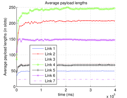
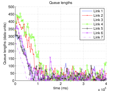
Let the “load” of arrival rates be ρ=0.8𝜌0.8\rho=0.8 (i.e., λ=0.8λ¯𝜆0.8¯𝜆{\bf\lambda}=0.8\cdot\bar{{\bf\lambda}}). The collision length (e.g., RTS length) is γ=5𝛾5\gamma=5, and the overhead of successful transmission is τ=10superscript𝜏10\tau^{\prime}=10. To show the negative drift of the queue lengths, assume that initially all queue lengths are 300 data units (where each data unit takes 100 slots to transmit). As expected, Fig. 7 (a) shows the convergence of the mean payload lengths, and Fig. 7 (b) shows that all queues are stable.
Refer to caption
(a) Convergence of the mean payload lengths
Refer to caption
(b) Stability of the queues
Figure 7: Simulation of Algorithm (17) (with the conflict graph in Fig. 6)
ρ𝜌\rho 0.65 0.7 0.75 0.8 0.85
Mean of D3subscript𝐷3D_{3} (in slots) 125.9 146.7 178.3 226.3 310.3
Standard deviation of D3subscript𝐷3D_{3} 132.7 161.9 211.5 293.7 456.1
TABLE I: Short-term fairness of link 3
R1subscript𝑅1R_{1} R2subscript𝑅2R_{2} R3subscript𝑅3R_{3} R4subscript𝑅4R_{4} R5subscript𝑅5R_{5} R6subscript𝑅6R_{6}
θ=0.15𝜃0.15\theta=0.15 (Simulation) 0.279 0.386 0.547 0.548 0.387 0.279
θ=0.15𝜃0.15\theta=0.15 ([28]) 0.272 0.347 0.442 0.442 0.347 0.273
θ=0.2𝜃0.2\theta=0.2 (Simulation) 0.526 0.837 1.372 1.371 0.840 0.526
θ=0.2𝜃0.2\theta=0.2 ([28]) 0.5 0.75 1.125 1.125 0.75 0.5
θ=0.25𝜃0.25\theta=0.25 (Simulation) 1.075 2.229 4.735 4.733 2.240 1.072
θ=0.25𝜃0.25\theta=0.25 ([28]) 1 2 4 4 2 1
θ=0.3𝜃0.3\theta=0.3 (Simulation) 3.210 12.94 52.76 52.32 12.91 3.209
θ=0.3𝜃0.3\theta=0.3 ([28]) 3 12 48 48 12 3
TABLE II: Comparison of access intensities

To study the tradeoff between the load ρ𝜌\rho and short-term fairness, we run Algorithm (17) for ρ{0.65,0.7,0.75,0.8,0.85}𝜌0.650.70.750.80.85\rho\in\{0.65,0.7,0.75,0.8,0.85\}. In each case, we collect the data of the access delay and compute its mean and standard deviation when 𝐫𝐫{\bf r} has almost converged. Table I shows the results for link 3 (and other links have a similar trend). Note that when ρ𝜌\rho increases, both the standard deviation and the mean increase, and their ratio increases too, indicating poorer short-term fairness.

In [28], van de Ven et al. considered the line topology (i.e., 1-D lattice topology) and obtained the explicit expression of the access intensity of each link required to support a uniform throughput θ𝜃\theta for all the links, under the idealized-CSMA model without collisions [14, 25, 26, 27]. For comparison, we simulate Algorithm 1 in a line topology with 6 links, where each link conflicts with the first 2 links on both sides. After Algorithm 1 converges, we compute the access intensity of link k𝑘k as Rk:=Tkp/(1/pk1)assignsubscript𝑅𝑘superscriptsubscript𝑇𝑘𝑝1subscript𝑝𝑘1R_{k}:=T_{k}^{p}/(1/p_{k}-1) (since the mean backoff time of link k𝑘k is 1/pk11subscript𝑝𝑘11/p_{k}-1), and compare it to the result of Theorem 2 in [28] (although the “access intensities” under the two models are not completely equivalent due to our inclusion of collisions.) Let pk=1/16,ksubscript𝑝𝑘116for-all𝑘p_{k}=1/16,\forall k, γ=1𝛾1\gamma=1 and τ=1superscript𝜏1\tau^{\prime}=1. We simulate four sets of arrival rates, λ=θ𝟏𝜆𝜃1{\bf\lambda}=\theta\cdot{\bf 1} where θ=0.15,0.2,0.25𝜃0.150.20.25\theta=0.15,0.2,0.25 and 0.30.30.3, and give the results in Table II.

The results show a close match, with relatively larger differences in R3subscript𝑅3R_{3} and R4subscript𝑅4R_{4}. The reason is that link 3 and 4 are in the middle of the network and suffer from more collisions. After each collision link 3 (or 4) needs to restart the backoff, which increases its effective backoff time and therefore requires a larger payload length to compensate. Also, all Rksubscript𝑅𝑘R_{k}’s are higher in the simulation due to collisions and the overhead τsuperscript𝜏\tau^{\prime}.

V-B Effect of dummy bits

We have used dummy bits to facilitate our analysis and design of the algorithms. However, transmitting dummy bits when a queue is empty consumes extra bandwidth. In this subsection, we simulate our algorithms without dummy bits.

In both Algorithm 1 and Algorithm (17), we make the following heuristic modification. For each link k𝑘k, if τkp(i)superscriptsubscript𝜏𝑘𝑝𝑖\tau_{k}^{p}(i) as computed in (15) is larger than the current (positive) queue length, then transmit a packet that includes all the bits of the queue as the payload. That is, no dummy bits are added. If the queue is empty then the link keeps silent. In the computation of sk(i)superscriptsubscript𝑠𝑘𝑖s_{k}^{\prime}(i), however, the payload of the packet is counted as τkp(i)superscriptsubscript𝜏𝑘𝑝𝑖\tau_{k}^{p}(i).777The reason for this design is that, if we only count the actual bits transmitted, then Algorithm (17) could not converge. Indeed, if Algorithm (17) converges, then the average service rates is strictly larger than the arrival rates, which is impossible if we only count the actually transmitted bits. Not surprisingly, the modified algorithms are difficult to analyze, and we therefore do not claim their convergence. (However, they still seem to converge in the simulations.)

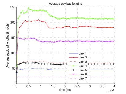
Fig. 8 shows the evolution of the average payload lengths under Algorithm (17) without dummy bits, when ρ=0.8𝜌0.8\rho=0.8. Indeed, the required payload lengths are significantly reduced compared to Fig. 7 (a) due to the saved bandwidth.

Under Algorithm 1, however, we find that the required payload lengths are very close with or without dummy bits. The reason is that, since Algorithm 1 only tries to make the average service rates equals the arrival rates, the queues do not have a negative drift towards zero. As a result, the queues are not close to zero most of the time, so dummy bits are rarely generated even if they are allowed.
Refer to caption
Figure 8: Algorithm (17) without dummy bits

V-C Effect of hidden nodes

So far we have assumed that there is no hidden node (HN) in the network. In this subsection we discuss the effect of HNs.

Consider a simple network with 2 links that are hidden from each other. That is, they cannot hear the transmissions of each other but a collision occurs if their transmissions overlap. Unlike the case without HNs, a link can start transmitting in the middle of the other link’s transmission and cause a collision.

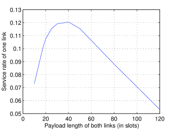
First, to explore how much service rates can be achieved in this scenario, we let the two links use the same, fixed payload length τpsuperscript𝜏𝑝\tau^{p}. Let γ=5,τ=10formulae-sequence𝛾5superscript𝜏10\gamma=5,\tau^{\prime}=10, and pk=1/64,ksubscript𝑝𝑘164for-all𝑘p_{k}=1/64,\forall k. The two links receive the same service rate by symmetry. Fig. 9 shows the service rate of one link under different values of τpsuperscript𝜏𝑝\tau^{p}. Note that the maximal service rate per link is about 0.12, much less than 0.5 in the case without HNs. Also, when τpsuperscript𝜏𝑝\tau^{p} is large enough, further increasing τpsuperscript𝜏𝑝\tau^{p} decreases the service rates, because larger packets are more easily collided by the HN.

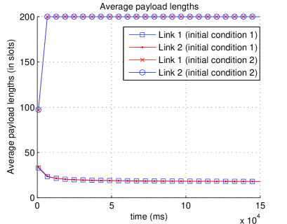
Then we simulate Algorithm 1 with arrival rates λ1=λ2=0.1<0.12subscript𝜆1subscript𝜆20.10.12\lambda_{1}=\lambda_{2}=0.1<0.12. We set T0=15,rmin=0,rmax=2.59formulae-sequencesubscript𝑇015formulae-sequencesubscript𝑟𝑚𝑖𝑛0subscript𝑟𝑚𝑎𝑥2.59T_{0}=15,r_{min}=0,r_{max}=2.59 so that the maximal payload is T0exp(rmax)=200subscript𝑇0subscript𝑟𝑚𝑎𝑥200T_{0}\exp(r_{max})=200 (slots), and α(i)=0.14/(2+i/100)𝛼𝑖0.142𝑖100\alpha(i)=0.14/(2+i/100). Unlike the case without HNs, the results depend on the initial condition as shown in Fig. 10. For example, if the initial payload lengths of both links are 40 slots (which we call “initial condition 1”), then the mean payload lengths converge to the correct value (about 17.5). However, if the initial payloads are 80 slots (“initial condition 2”), then the mean payload lengths keep increasing (until reaching the maximal value) and cannot support the arrival rates. This can be explained by Fig. 9. Initial payload lengths of 40 slots achieve a per-link service rate higher than the arrival rate. By Algorithm 1, the payload lengths are decreased and eventually converge to the correct values. However, if initially the payload lengths are 80 slots, a per-link service rate lower than 0.1 is achieved. By Algorithm 1, both links increase their payload lengths. This, however, further decreases their service rates, and the cycle goes on. The root cause for this behavior is as follows. Algorithm 1 has implicitly used the fact that, without HNs, a link’s service rate increases with its payload length. However, it may not be the case when HNs exist.

To sum up, in the presence of HNs, both the achievable capacity region of CSMA and the property of our algorithms have changed. To address the HN problem, there are at least two directions to explore. The first is to understand the achievable capacity with HNs, and design algorithms to achieve the capacity. The second is to design protocols to remove or reduce HNs, so that our existing algorithms can be applied. There have been many proposals aiming to remove or reduce the HNs (see [19] and the references therein).
Refer to caption
Figure 9: Service rates in a 2-link network with hidden nodes
Refer to caption
Figure 10: Algorithm 1 with hidden nodes

VI Conclusion

In this paper, we have studied CSMA-based scheduling algorithms with collisions. We first provided a model and gave a throughput formula which takes into account the cost of collisions and overhead. The formula has a simple product form. Next, we designed distributed algorithms where each link adaptively updates its mean transmission length to approach the throughput-optimality, and provided sufficient conditions to ensure the convergence and stability of the algorithms. We also characterized the relationship between the algorithm parameters and the achievable capacity region. Finally, simulations results were presented to illustrate and verify the main results.

In the algorithm, the transmission probabilities of the links are chosen to be fixed at a reasonable level, since we have shown that adjusting the transmission lengths alone is sufficient to approach throughput-optimality (the main goal of this paper). However, the choices of the transmission probabilities pksubscript𝑝𝑘p_{k}’s has an effect on the probability of collisions among the probe packets. In the future, we would like to further study whether the adjustment of transmission probabilities can be combined with the algorithm. Also, we are interested to further explore the short-term fairness and the case with hidden nodes.

Appendix A Proofs of theorems

A-A Proof of Theorem 1

First, the stationary distribution of the CSMA/CA Markov chain is expressed in the following lemma.

Lemma 1

In the stationary distribution, the probability of a valid state w𝑤w as defined by (3) is

p(w)=1Ei:xi=0qij:xj=1[pjf(bj,j,x)]𝑝𝑤1𝐸subscriptproduct:𝑖subscript𝑥𝑖0subscript𝑞𝑖subscriptproduct:𝑗subscript𝑥𝑗1delimited-[]subscript𝑝𝑗𝑓subscript𝑏𝑗𝑗𝑥p(w)=\frac{1}{E}\prod_{i:x_{i}=0}q_{i}\prod_{j:x_{j}=1}[p_{j}\cdot f(b_{j},j,x)] (22)

where

f(bj,j,x)={1if jZ(x)Pj(bj)if jS(x),𝑓subscript𝑏𝑗𝑗𝑥cases1if 𝑗𝑍𝑥subscript𝑃𝑗subscript𝑏𝑗if 𝑗𝑆𝑥f(b_{j},j,x)=\begin{cases}1&\text{if }j\in Z(x)\\ P_{j}(b_{j})&\text{if }j\in S(x)\end{cases}, (23)

where Pj(bj)subscript𝑃𝑗subscript𝑏𝑗P_{j}(b_{j}) is the p.m.f. of link j𝑗j’s transmission length, as defined in (1). Also, E𝐸E is a normalizing term such that wp(w)=1subscript𝑤𝑝𝑤1\sum_{w}p(w)=1, i.e., all probabilities sum up to 1. Note that p(w)𝑝𝑤p(w) does not depend on the remaining time aksubscript𝑎𝑘a_{k}’s.

Proof:

For a given state w={x,((bk,ak),k:xk=1)}w=\{x,((b_{k},a_{k}),\forall k:x_{k}=1)\}, define the set of active links whose remaining time is larger than 1 as

A1(w)={k|xk=1,ak>1}.subscript𝐴1𝑤conditional-set𝑘formulae-sequencesubscript𝑥𝑘1subscript𝑎𝑘1A_{1}(w)=\{k|x_{k}=1,a_{k}>1\}.

Links in A1(w)subscript𝐴1𝑤A_{1}(w) will continue their transmissions (either with success or a collision) in the next slot.

Define the set of inactive links “blocked” by links in A1(w)subscript𝐴1𝑤A_{1}(w) as

A1(w)={j|xj=0;e(j,k)=1 for some kA1(w)}subscript𝐴1𝑤conditional-set𝑗formulae-sequencesubscript𝑥𝑗0𝑒𝑗𝑘1 for some 𝑘subscript𝐴1𝑤\partial A_{1}(w)=\{j|x_{j}=0;e(j,k)=1\text{ for some }k\in A_{1}(w)\}

where e(j,k)=1𝑒𝑗𝑘1e(j,k)=1 means that there is an edge between j𝑗j and k𝑘k in the conflict graph. Links in A1(w)subscript𝐴1𝑤\partial A_{1}(w) will remain inactive in the next slot.

Write A¯1(w):=A1(w)A1(w)assignsubscript¯𝐴1𝑤subscript𝐴1𝑤subscript𝐴1𝑤\bar{A}_{1}(w):=A_{1}(w)\cup\partial A_{1}(w). Define the set of all other links as

A2(w)=𝒩\A¯1(w).subscript𝐴2𝑤\𝒩subscript¯𝐴1𝑤A_{2}(w)={\cal N}\backslash\bar{A}_{1}(w). (24)

These links can change their on-off states xksubscript𝑥𝑘x_{k}’s in the next slot. On the other hand, links in A¯1(w)subscript¯𝐴1𝑤\bar{A}_{1}(w) will have the same on-off states xksubscript𝑥𝑘x_{k}’s in the next slot.

To illustrate these notations, consider the example in Fig. 5. By (4), we have A1(w)={3},A1(w)={2},A¯1(w)={2,3}formulae-sequencesubscript𝐴1𝑤3formulae-sequencesubscript𝐴1𝑤2subscript¯𝐴1𝑤23A_{1}(w)=\{3\},\partial A_{1}(w)=\{2\},\bar{A}_{1}(w)=\{2,3\} and A2(w)={1}subscript𝐴2𝑤1A_{2}(w)=\{1\}.

State w𝑤w can transit in the next slot to another valid state w={x,((bk,ak),k:xk=1)}w^{\prime}=\{x^{\prime},((b_{k}^{\prime},a_{k}^{\prime}),\forall k:x_{k}^{\prime}=1)\}, i.e., Q(w,w)>0𝑄𝑤superscript𝑤0Q(w,w^{\prime})>0, if and only if wsuperscript𝑤w^{\prime} satisfies that (i) xk=xk,kA¯1(w)formulae-sequencesuperscriptsubscript𝑥𝑘subscript𝑥𝑘for-all𝑘subscript¯𝐴1𝑤x_{k}^{\prime}=x_{k},\forall k\in\bar{A}_{1}(w); (ii) bk=bk,ak=ak1,kA¯1(w) such that xk=1formulae-sequencesuperscriptsubscript𝑏𝑘subscript𝑏𝑘formulae-sequencesuperscriptsubscript𝑎𝑘subscript𝑎𝑘1for-all𝑘subscript¯𝐴1𝑤 such that subscript𝑥𝑘1b_{k}^{\prime}=b_{k},a_{k}^{\prime}=a_{k}-1,\forall k\in\bar{A}_{1}(w)\text{ such that }x_{k}=1; (iii) ak=bk,kA2(w) such that xk=1formulae-sequencesuperscriptsubscript𝑎𝑘superscriptsubscript𝑏𝑘for-all𝑘subscript𝐴2𝑤 such that superscriptsubscript𝑥𝑘1a_{k}^{\prime}=b_{k}^{\prime},\forall k\in A_{2}(w)\text{ such that }x_{k}^{\prime}=1, and bk=γ,kA2(w)Z(x)formulae-sequencesuperscriptsubscript𝑏𝑘𝛾for-all𝑘subscript𝐴2𝑤𝑍superscript𝑥b_{k}^{\prime}=\gamma,\forall k\in A_{2}(w)\cap Z(x^{\prime}). (If A2(w)subscript𝐴2𝑤A_{2}(w) is an empty set, then condition (iii) is trivially true.) The transition probability is

Q(w,w)=iA2(w)[pif(bi,i,x)]xiqi1xi.𝑄𝑤superscript𝑤subscriptproduct𝑖subscript𝐴2𝑤superscriptdelimited-[]subscript𝑝𝑖𝑓superscriptsubscript𝑏𝑖𝑖superscript𝑥superscriptsubscript𝑥𝑖superscriptsubscript𝑞𝑖1superscriptsubscript𝑥𝑖Q(w,w^{\prime})=\prod_{i\in A_{2}(w)}[p_{i}\cdot f(b_{i}^{\prime},i,x^{\prime})]^{x_{i}^{\prime}}q_{i}^{1-x_{i}^{\prime}}. (25)

Define

Q~(w,w):=iA2(w)[pif(bi,i,x)]xiqi1xi.assign~𝑄superscript𝑤𝑤subscriptproduct𝑖subscript𝐴2𝑤superscriptdelimited-[]subscript𝑝𝑖𝑓subscript𝑏𝑖𝑖𝑥subscript𝑥𝑖superscriptsubscript𝑞𝑖1subscript𝑥𝑖\tilde{Q}(w^{\prime},w):=\prod_{i\in A_{2}(w)}[p_{i}\cdot f(b_{i},i,x)]^{x_{i}}q_{i}^{1-x_{i}}. (26)

(If A2(w)subscript𝐴2𝑤A_{2}(w) is an empty set, then Q(w,w)=1𝑄𝑤superscript𝑤1Q(w,w^{\prime})=1 and Q~(w,w):=1assign~𝑄superscript𝑤𝑤1\tilde{Q}(w^{\prime},w):=1.) If w𝑤w and wsuperscript𝑤w^{\prime} does not satisfy all the conditions (i), (ii), (iii), then Q(w,w)=0𝑄𝑤superscript𝑤0Q(w,w^{\prime})=0, and also define Q~(w,w)=0~𝑄superscript𝑤𝑤0\tilde{Q}(w^{\prime},w)=0.

Then, if Q(w,w)>0𝑄𝑤superscript𝑤0Q(w,w^{\prime})>0 (and Q~(w,w)>0~𝑄superscript𝑤𝑤0\tilde{Q}(w^{\prime},w)>0), p(w)/Q~(w,w)=1EiA2(w)[pif(bi,i,x)]xiqi1xi𝑝𝑤~𝑄superscript𝑤𝑤1𝐸subscriptproduct𝑖subscript𝐴2𝑤superscriptdelimited-[]subscript𝑝𝑖𝑓subscript𝑏𝑖𝑖𝑥subscript𝑥𝑖superscriptsubscript𝑞𝑖1subscript𝑥𝑖p(w)/\tilde{Q}(w^{\prime},w)=\frac{1}{E}\prod_{i\notin A_{2}(w)}[p_{i}\cdot f(b_{i},i,x)]^{x_{i}}q_{i}^{1-x_{i}}. And p(w)/Q(w,w)=1EiA2(w)[pif(bi,i,x)]xiqi1xi𝑝superscript𝑤𝑄𝑤superscript𝑤1𝐸subscriptproduct𝑖subscript𝐴2𝑤superscriptdelimited-[]subscript𝑝𝑖𝑓superscriptsubscript𝑏𝑖𝑖superscript𝑥superscriptsubscript𝑥𝑖superscriptsubscript𝑞𝑖1superscriptsubscript𝑥𝑖p(w^{\prime})/Q(w,w^{\prime})=\frac{1}{E}\prod_{i\notin A_{2}(w)}[p_{i}\cdot f(b_{i}^{\prime},i,x^{\prime})]^{x_{i}^{\prime}}q_{i}^{1-x_{i}^{\prime}}. But for any iA2(w)𝑖subscript𝐴2𝑤i\notin A_{2}(w), i.e., iA¯1(w)𝑖subscript¯𝐴1𝑤i\in\bar{A}_{1}(w), we have xi=xi,bi=biformulae-sequencesuperscriptsubscript𝑥𝑖subscript𝑥𝑖superscriptsubscript𝑏𝑖subscript𝑏𝑖x_{i}^{\prime}=x_{i},b_{i}^{\prime}=b_{i} by condition (i), (ii) above. Therefore, the two expressions are equal. Thus

p(w)Q(w,w)=p(w)Q~(w,w).𝑝𝑤𝑄𝑤superscript𝑤𝑝superscript𝑤~𝑄superscript𝑤𝑤p(w)Q(w,w^{\prime})=p(w^{\prime})\tilde{Q}(w^{\prime},w). (27)

If two states w,w𝑤superscript𝑤w,w^{\prime} satisfy Q(w,w)=0𝑄𝑤superscript𝑤0Q(w,w^{\prime})=0, then by definition Q~(w,w)=0~𝑄superscript𝑤𝑤0\tilde{Q}(w^{\prime},w)=0, making (27) trivially true. Therefore, (27) holds for any w𝑤w and wsuperscript𝑤w^{\prime}.

We will show later that Q~(w,w)~𝑄superscript𝑤𝑤\tilde{Q}(w^{\prime},w) is the transition probability of the “time-reversed process” of the above Markov chain (notice the similarity between Q(w,w)𝑄𝑤superscript𝑤Q(w,w^{\prime}) and Q~(w,w)~𝑄superscript𝑤𝑤\tilde{Q}(w^{\prime},w)), and naturally satisfies wQ~(w,w)=1subscript𝑤~𝑄superscript𝑤𝑤1\sum_{w}\tilde{Q}(w^{\prime},w)=1. Assuming that the claim is true, then by (27), we have

wp(w)Q(w,w)=p(w)wQ~(w,w)=p(w).subscript𝑤𝑝𝑤𝑄𝑤superscript𝑤𝑝superscript𝑤subscript𝑤~𝑄superscript𝑤𝑤𝑝superscript𝑤\sum_{w}p(w)\cdot Q(w,w^{\prime})=p(w^{\prime})\sum_{w}\tilde{Q}(w^{\prime},w)=p(w^{\prime}).

Therefore, p(w)𝑝𝑤p(w) is the stationary (or “invariant”) distribution, which completes the proof of Lemma 1.

It remains to be shown that the above claim is true, in particular, that wQ~(w,w)=1subscript𝑤~𝑄superscript𝑤𝑤1\sum_{w}\tilde{Q}(w^{\prime},w)=1. Denote the orignal process as {w(t),t𝒵}𝑤𝑡𝑡𝒵\{w(t),t\in{\cal Z}\} (this is the Markov process that describes our CSMA protocol, with transition probabilities Q(,)𝑄Q(\cdot,\cdot) in (25)). Adding a time index in (3), we have

w(t):={x(t),((bk(t),ak(t)),k:xk(t)=1)}.w(t):=\{x(t),((b_{k}(t),a_{k}(t)),\forall k:x_{k}(t)=1)\}. (28)

Now define the time-reversed process w~(t):=w(t),t𝒵formulae-sequenceassign~𝑤𝑡𝑤𝑡for-all𝑡𝒵\tilde{w}(t):=w(-t),\forall t\in{\cal Z}. First, note that in the process {w(t)}𝑤𝑡\{w(t)\}, the remaining time ak(t)subscript𝑎𝑘𝑡a_{k}(t), if defined, decreases with t𝑡t; in the reversed process {w~(t)}~𝑤𝑡\{\tilde{w}(t)\}, however, ak(t)subscript𝑎𝑘𝑡a_{k}(-t) increases with t𝑡t. Therefore, {w(t)}𝑤𝑡\{w(t)\} and {w~(t)}~𝑤𝑡\{\tilde{w}(t)\} are, clearly, statistically distinguishable. So {w(t)}𝑤𝑡\{w(t)\} is not time-reversible.

However, if we re-label the “remaining time” in the reversed order, then the process {w~(t)}~𝑤𝑡\{\tilde{w}(t)\} “looks a lot” like the process {w(t)}𝑤𝑡\{w(t)\}. (This is why we say the CSMA/CA Markov chain is almost time-reversible.) More formally, with the understanding that w={x,((bk,ak),k:xk=1)}w=\{x,((b_{k},a_{k}),\forall k:x_{k}=1)\}, define a function g()𝑔g(\cdot) as

g(w)={x,((bk,bkak+1),k:xk=1)}.g(w)=\{x,((b_{k},b_{k}-a_{k}+1),\forall k:x_{k}=1)\}. (29)

Then define the process

w^(t):=g(w(t)).assign^𝑤𝑡𝑔𝑤𝑡\hat{w}(t):=g(w(-t)).

Note that in the process {w^(t)}^𝑤𝑡\{\hat{w}(t)\}, the “remaining time” decreases with t𝑡t, similar to {w(t)}𝑤𝑡\{w(t)\}.

Next we show the following two facts.

Fact 1: For any two states w𝑤w and wsuperscript𝑤w^{\prime} with Q(w,w)>0𝑄𝑤superscript𝑤0Q(w,w^{\prime})>0 (i.e., if the CSMA Markov chain can transit from state w𝑤w to state wsuperscript𝑤w^{\prime}), we have A1(w)=A1(g(w))subscript𝐴1𝑤subscript𝐴1𝑔superscript𝑤A_{1}(w)=A_{1}(g(w^{\prime})), A¯1(w)=A¯1(g(w))subscript¯𝐴1𝑤subscript¯𝐴1𝑔superscript𝑤\bar{A}_{1}(w)=\bar{A}_{1}(g(w^{\prime})) and A2(w)=A2(g(w))subscript𝐴2𝑤subscript𝐴2𝑔superscript𝑤A_{2}(w)=A_{2}(g(w^{\prime})).

Fact 2: Q(w,w)>0Q(g(w),g(w))>0𝑄𝑤superscript𝑤0𝑄𝑔superscript𝑤𝑔𝑤0Q(w,w^{\prime})>0\Leftrightarrow Q(g(w^{\prime}),g(w))>0.

These facts can be illustrated by the example in Fig. 5. First consider Fact 1. Note that A1(w)={3}subscript𝐴1𝑤3A_{1}(w)=\{3\}, by definition, is the set of links that are in the middle of a transmission in state w𝑤w and will continue the transmission in the next state wsuperscript𝑤w^{\prime}. Then, in the reversed process, such links are also in the middle of a transmission in state g(w)𝑔superscript𝑤g(w^{\prime}) and will continue the transmission in the next state g(w)𝑔𝑤g(w). So A1(w)=A1(g(w))subscript𝐴1𝑤subscript𝐴1𝑔superscript𝑤A_{1}(w)=A_{1}(g(w^{\prime})). Similarly, A1(w)={2}subscript𝐴1𝑤2\partial A_{1}(w)=\{2\}, the set of links that are blocked by A1(w)subscript𝐴1𝑤A_{1}(w) in w𝑤w are also blocked by A1(g(w))subscript𝐴1𝑔superscript𝑤A_{1}(g(w^{\prime})) in the reversed process. Therefore A1(w)=A1(g(w))subscript𝐴1𝑤subscript𝐴1𝑔superscript𝑤\partial A_{1}(w)=\partial A_{1}(g(w^{\prime})). Then by (24), we have A2(w)=A2(g(w))subscript𝐴2𝑤subscript𝐴2𝑔superscript𝑤A_{2}(w)=A_{2}(g(w^{\prime})). (Note that it is not difficult to prove Fact 1 mechanically via the definitions of A1(),A2()subscript𝐴1subscript𝐴2A_{1}(\cdot),A_{2}(\cdot). But we omit it here.)

One can also verify Fact 2 in Fig. 5. We now give a more formal proof. If Q(w,w)>0𝑄𝑤superscript𝑤0Q(w,w^{\prime})>0, then w𝑤w and wsuperscript𝑤w^{\prime} satisfy conditions (i)~(iii). We first show that Q(g(w),g(w))>0𝑄𝑔superscript𝑤𝑔𝑤0Q(g(w^{\prime}),g(w))>0. To this end, we need to verify that the states g(w)𝑔superscript𝑤g(w^{\prime}) and g(w)𝑔𝑤g(w) satisfy condition (i)~(iii). Condition (i) holds because A¯1(w)=A¯1(g(w))subscript¯𝐴1𝑤subscript¯𝐴1𝑔superscript𝑤\bar{A}_{1}(w)=\bar{A}_{1}(g(w^{\prime})) by Fact 1, and because g()𝑔g(\cdot) does not change the “on-off state” of its argument. Condition (ii) holds since g()𝑔g(\cdot) has reversed the remaining time (cf. (29)). Condition (iii) requires that in the reversed process, any link kA2(g(w))𝑘subscript𝐴2𝑔superscript𝑤k\in A_{2}(g(w^{\prime})) which is transmitting in the state g(w)𝑔𝑤g(w) must have just started its transmission. This is true because A2(g(w))=A2(w)subscript𝐴2𝑔superscript𝑤subscript𝐴2𝑤A_{2}(g(w^{\prime}))=A_{2}(w) by Fact 1, and that in the original process w(t)𝑤𝑡w(t), any link kA2(w)𝑘subscript𝐴2𝑤k\in A_{2}(w) which is transmitting in state w𝑤w must be in its last slot of the transmission (otherwise the link would be in A1(w)subscript𝐴1𝑤A_{1}(w)). Then condition (iii) holds since g()𝑔g(\cdot) has reversed the remaining time.

This completes the proof that Q(w,w)>0Q(g(w),g(w))>0𝑄𝑤superscript𝑤0𝑄𝑔superscript𝑤𝑔𝑤0Q(w,w^{\prime})>0\Rightarrow Q(g(w^{\prime}),g(w))>0. Now, if Q(g(w),g(w))>0𝑄𝑔superscript𝑤𝑔𝑤0Q(g(w^{\prime}),g(w))>0, by the above result, we have Q(g(g(w)),g(g(w)))>0𝑄𝑔𝑔𝑤𝑔𝑔superscript𝑤0Q(g(g(w)),g(g(w^{\prime})))>0. Since g(g(w))=w,g(g(w))=wformulae-sequence𝑔𝑔𝑤𝑤𝑔𝑔superscript𝑤superscript𝑤g(g(w))=w,g(g(w^{\prime}))=w^{\prime}, we have Q(w,w)>0𝑄𝑤superscript𝑤0Q(w,w^{\prime})>0. This completes the proof of Fact 2.

Consider two states w𝑤w and wsuperscript𝑤w^{\prime} with Q(w,w)>0𝑄𝑤superscript𝑤0Q(w,w^{\prime})>0. Then Q(g(w),g(w))>0𝑄𝑔superscript𝑤𝑔𝑤0Q(g(w^{\prime}),g(w))>0, with

Q(g(w),g(w))=iA2(g(w))[pif(bi,i,x)]xiqi1xi𝑄𝑔superscript𝑤𝑔𝑤subscriptproduct𝑖subscript𝐴2𝑔superscript𝑤superscriptdelimited-[]subscript𝑝𝑖𝑓subscript𝑏𝑖𝑖𝑥subscript𝑥𝑖superscriptsubscript𝑞𝑖1subscript𝑥𝑖Q(g(w^{\prime}),g(w))=\prod_{i\in A_{2}(g(w^{\prime}))}[p_{i}\cdot f(b_{i},i,x)]^{x_{i}}q_{i}^{1-x_{i}}

by (25). Using (26) and A2(w)=A2(g(w))subscript𝐴2𝑤subscript𝐴2𝑔superscript𝑤A_{2}(w)=A_{2}(g(w^{\prime})), we have

Q~(w,w)~𝑄superscript𝑤𝑤\displaystyle\tilde{Q}(w^{\prime},w) =\displaystyle= iA2(w)[pif(bi,i,x)]xiqi1xisubscriptproduct𝑖subscript𝐴2𝑤superscriptdelimited-[]subscript𝑝𝑖𝑓subscript𝑏𝑖𝑖𝑥subscript𝑥𝑖superscriptsubscript𝑞𝑖1subscript𝑥𝑖\displaystyle\prod_{i\in A_{2}(w)}[p_{i}\cdot f(b_{i},i,x)]^{x_{i}}q_{i}^{1-x_{i}} (30)
=\displaystyle= iA2(g(w))[pif(bi,i,x)]xiqi1xisubscriptproduct𝑖subscript𝐴2𝑔superscript𝑤superscriptdelimited-[]subscript𝑝𝑖𝑓subscript𝑏𝑖𝑖𝑥subscript𝑥𝑖superscriptsubscript𝑞𝑖1subscript𝑥𝑖\displaystyle\prod_{i\in A_{2}(g(w^{\prime}))}[p_{i}\cdot f(b_{i},i,x)]^{x_{i}}q_{i}^{1-x_{i}}
=\displaystyle= Q(g(w),g(w)).𝑄𝑔superscript𝑤𝑔𝑤\displaystyle Q(g(w^{\prime}),g(w)).

Therefore, Q~(w,w)~𝑄superscript𝑤𝑤\tilde{Q}(w^{\prime},w) is the transition probability of the reversed process.

By definition, Q~(w,w)=0~𝑄superscript𝑤𝑤0\tilde{Q}(w^{\prime},w)=0 for any w,w𝑤superscript𝑤w,w^{\prime} satisfying Q(w,w)=0𝑄𝑤superscript𝑤0Q(w,w^{\prime})=0. So, given wsuperscript𝑤w^{\prime},

wQ~(w,w)subscript𝑤~𝑄superscript𝑤𝑤\displaystyle\sum_{w}\tilde{Q}(w^{\prime},w) =\displaystyle= w:Q(w,w)>0Q~(w,w)subscript:𝑤𝑄𝑤superscript𝑤0~𝑄superscript𝑤𝑤\displaystyle\sum_{w:Q(w,w^{\prime})>0}\tilde{Q}(w^{\prime},w)
=\displaystyle= w:Q(w,w)>0Q(g(w),g(w))subscript:𝑤𝑄𝑤superscript𝑤0𝑄𝑔superscript𝑤𝑔𝑤\displaystyle\sum_{w:Q(w,w^{\prime})>0}Q(g(w^{\prime}),g(w))
=\displaystyle= w:Q(g(w),g(w))>0Q(g(w),g(w))subscript:𝑤𝑄𝑔superscript𝑤𝑔𝑤0𝑄𝑔superscript𝑤𝑔𝑤\displaystyle\sum_{w:Q(g(w^{\prime}),g(w))>0}Q(g(w^{\prime}),g(w))
=\displaystyle= wQ(g(w),g(w))=1subscript𝑤𝑄𝑔superscript𝑤𝑔𝑤1\displaystyle\sum_{w}Q(g(w^{\prime}),g(w))=1

where the last step has used the fact that g()𝑔g(\cdot) is a one-one mapping, so that the summation is over all valid states. ∎

Using Lemma 1, the probability of any on-off state x𝑥x, as in Theorem 1, can be computed by summing up the probabilities of all states w𝑤w’s with the same on-off state x𝑥x, using (22).

Define the set of valid states (x):={w| the on-off state is x in the state w}assign𝑥conditional-set𝑤 the on-off state is 𝑥 in the state 𝑤{\cal B}(x):=\{w|\text{ the on-off state is }x\text{ in the state }w\}. By Lemma 1, we have

p(x)=w(x)p(w)𝑝𝑥subscript𝑤𝑥𝑝𝑤\displaystyle p(x)=\sum_{w\in{\cal B}(x)}p(w) (31)
=\displaystyle= 1Ew(x){i:xi=0qij:xj=1[pjf(bj,j,x)]}1𝐸subscript𝑤𝑥subscriptproduct:𝑖subscript𝑥𝑖0subscript𝑞𝑖subscriptproduct:𝑗subscript𝑥𝑗1delimited-[]subscript𝑝𝑗𝑓subscript𝑏𝑗𝑗𝑥\displaystyle\frac{1}{E}\sum_{w\in{\cal B}(x)}\{\prod_{i:x_{i}=0}q_{i}\prod_{j:x_{j}=1}[p_{j}\cdot f(b_{j},j,x)]\}
=\displaystyle= 1E(i:xi=0qij:xj=1pj)w(x)j:xj=1f(bj,j,x)1𝐸subscriptproduct:𝑖subscript𝑥𝑖0subscript𝑞𝑖subscriptproduct:𝑗subscript𝑥𝑗1subscript𝑝𝑗subscript𝑤𝑥subscriptproduct:𝑗subscript𝑥𝑗1𝑓subscript𝑏𝑗𝑗𝑥\displaystyle\frac{1}{E}(\prod_{i:x_{i}=0}q_{i}\prod_{j:x_{j}=1}p_{j})\sum_{w\in{\cal B}(x)}\prod_{j:x_{j}=1}f(b_{j},j,x)
=\displaystyle= 1E(i:xi=0qij:xj=1pj)w(x)[jS(x)Pj(bj)].1𝐸subscriptproduct:𝑖subscript𝑥𝑖0subscript𝑞𝑖subscriptproduct:𝑗subscript𝑥𝑗1subscript𝑝𝑗subscript𝑤𝑥delimited-[]subscriptproduct𝑗𝑆𝑥subscript𝑃𝑗subscript𝑏𝑗\displaystyle\frac{1}{E}(\prod_{i:x_{i}=0}q_{i}\prod_{j:x_{j}=1}p_{j})\cdot\sum_{w\in{\cal B}(x)}[\prod_{j\in S(x)}P_{j}(b_{j})].

Now we compute the term w(x)[jS(x)Pj(bj)]subscript𝑤𝑥delimited-[]subscriptproduct𝑗𝑆𝑥subscript𝑃𝑗subscript𝑏𝑗\sum_{w\in{\cal B}(x)}[\prod_{j\in S(x)}P_{j}(b_{j})]. Consider a state w={x,((bk,ak),k:xk=1)}(x)w=\{x,((b_{k},a_{k}),\forall k:x_{k}=1)\}\in{\cal B}(x). For kS(x)𝑘𝑆𝑥k\in S(x), bksubscript𝑏𝑘b_{k} can take different values in 𝒵++subscript𝒵absent{\cal Z}_{++}. For each fixed bksubscript𝑏𝑘b_{k}, aksubscript𝑎𝑘a_{k} can be any integer from 1 to bksubscript𝑏𝑘b_{k}. For a collision component Cm(x)subscript𝐶𝑚𝑥C_{m}(x) (i.e., |Cm(x)|>1subscript𝐶𝑚𝑥1|C_{m}(x)|>1), the remaining time of each link in the component, a(m)superscript𝑎𝑚a^{(m)}, can be any integer from 1 to γ𝛾\gamma. Then we have

w(x)[jS(x)Pj(bj)]subscript𝑤𝑥delimited-[]subscriptproduct𝑗𝑆𝑥subscript𝑃𝑗subscript𝑏𝑗\displaystyle\sum_{w\in{\cal B}(x)}[\prod_{j\in S(x)}P_{j}(b_{j})] (32)
=\displaystyle= jS(x)[bj1ajbjPj(bj)]m:|Cm(x)|>1(1a(m)γ1)subscriptproduct𝑗𝑆𝑥delimited-[]subscriptsubscript𝑏𝑗subscript1subscript𝑎𝑗subscript𝑏𝑗subscript𝑃𝑗subscript𝑏𝑗subscriptproduct:𝑚subscript𝐶𝑚𝑥1subscript1superscript𝑎𝑚𝛾1\displaystyle\prod_{j\in S(x)}[\sum_{b_{j}}\sum_{1\leq a_{j}\leq b_{j}}P_{j}(b_{j})]\prod_{m:|C_{m}(x)|>1}(\sum_{1\leq a^{(m)}\leq\gamma}1)
=\displaystyle= jS(x)[bjbjPj(bj)]γh(x)subscriptproduct𝑗𝑆𝑥delimited-[]subscriptsubscript𝑏𝑗subscript𝑏𝑗subscript𝑃𝑗subscript𝑏𝑗superscript𝛾𝑥\displaystyle\prod_{j\in S(x)}[\sum_{b_{j}}b_{j}P_{j}(b_{j})]\cdot\gamma^{h(x)}
=\displaystyle= (jS(x)Tj)γh(x).subscriptproduct𝑗𝑆𝑥subscript𝑇𝑗superscript𝛾𝑥\displaystyle(\prod_{j\in S(x)}T_{j})\gamma^{h(x)}.

Combining (31) and (32) completes the proof.

A-B Proof of Theorem 2

A-B1 Some definitions

If at an on-off state x𝑥x, kS(x)𝑘𝑆𝑥k\in S(x) (i.e., k𝑘k is transmitting successfully), it is possible that link k𝑘k is transmitting the overhead or the payload. So we define the “detailed state” (x,z)𝑥𝑧(x,z), where z{0,1}K𝑧superscript01𝐾z\in\{0,1\}^{K}. Let zk=1subscript𝑧𝑘1z_{k}=1 if kS(x)𝑘𝑆𝑥k\in S(x) and link k𝑘k is transmitting its payload (instead of overhead). Let zk=0subscript𝑧𝑘0z_{k}=0 otherwise. Denote the set of all possible detailed states (x,z)𝑥𝑧(x,z) by 𝒮𝒮{\cal S}.

Then similar to the proof of Theorem 1, and using equation (7), we have the following product-form stationary distribution

p((x,z);𝐫)=1E(𝐫)g(x,z)exp(kzkrk)𝑝𝑥𝑧𝐫1𝐸𝐫𝑔𝑥𝑧subscript𝑘subscript𝑧𝑘subscript𝑟𝑘p((x,z);{\bf r})=\frac{1}{E({\bf r})}g(x,z)\cdot\exp(\sum_{k}z_{k}r_{k}) (33)

where

g(x,z)=g(x)(τ)|S(x)|𝟏𝐳T0𝟏𝐳𝑔𝑥𝑧𝑔𝑥superscriptsuperscript𝜏𝑆𝑥superscript1𝐳superscriptsubscript𝑇0superscript1𝐳g(x,z)=g(x)\cdot(\tau^{\prime})^{|S(x)|-{\bf 1}^{\prime}{\bf z}}T_{0}^{{\bf 1}^{\prime}{\bf z}} (34)

where 𝟏𝐳superscript1𝐳{\bf 1}^{\prime}{\bf z} is the number of links that are transmitting the payload in state (x,z)𝑥𝑧(x,z).

Clearly, this provides another expression of the service rate sk(𝐫)subscript𝑠𝑘𝐫s_{k}({\bf r}):

sk(𝐫)=(x,z)𝒮:zk=1p((x,z);𝐫).subscript𝑠𝑘𝐫subscript:𝑥𝑧𝒮subscript𝑧𝑘1𝑝𝑥𝑧𝐫s_{k}({\bf r})=\sum_{(x,z)\in{\cal S}:z_{k}=1}p((x,z);{\bf r}). (35)

Now we give alternative definitions of feasible and strictly feasible arrival rates to facilitate our proof. We will show that these definitions are equivalent to Definition 1.

Definition 2

(i) A vector of arrival rate λ+K𝜆superscriptsubscript𝐾{\bf\lambda}\in{\cal R}_{+}^{K} (where K𝐾K is the number of links) is feasible if there exists a probability distribution 𝐩¯¯𝐩\bar{{\bf p}} over 𝒮𝒮{\cal S} (i.e., (x,z)𝒮p¯((x,z))=1subscript𝑥𝑧𝒮¯𝑝𝑥𝑧1\sum_{(x,z)\in{\cal S}}\bar{p}((x,z))=1 and p¯((x,z))0¯𝑝𝑥𝑧0\bar{p}((x,z))\geq 0), such that

λk=(x,z)𝒮p¯((x,z))zk.subscript𝜆𝑘subscript𝑥𝑧𝒮¯𝑝𝑥𝑧subscript𝑧𝑘\lambda_{k}=\sum_{(x,z)\in{\cal S}}\bar{p}((x,z))\cdot z_{k}. (36)

Let 𝒞¯COsubscript¯𝒞𝐶𝑂\bar{{\cal C}}_{CO} be the set of feasible λ𝜆{\bf\lambda}, where “CO” stands for “collision”.

The rationale of the definition is that if λ𝜆{\bf\lambda} can be scheduled by the network, the fraction of time that the network spent in the detailed states must be non-negative and sum up to 1. (Note that (36) is the probability that link k𝑘k is sending its payload given the distribution of the detailed states.)

(ii) A vector of arrival rate λ+K𝜆superscriptsubscript𝐾{\bf\lambda}\in{\cal R}_{+}^{K} is strictly feasible if it can be written as (36) where (x,z)𝒮p¯((x,z))=1subscript𝑥𝑧𝒮¯𝑝𝑥𝑧1\sum_{(x,z)\in{\cal S}}\bar{p}((x,z))=1 and p¯((x,z))>0¯𝑝𝑥𝑧0\bar{p}((x,z))>0. Let 𝒞COsubscript𝒞𝐶𝑂{\cal C}_{CO} be the set of strictly feasible λ𝜆{\bf\lambda}.

For example, in the ad-hoc network in Fig. 2 (b), λ=(0.5,0.5,0.5)𝜆0.50.50.5{\bf\lambda}=(0.5,0.5,0.5) is feasible, because (36) holds if we let the probability of the detailed state (x=(1,0,1),z=(1,0,1))formulae-sequence𝑥101𝑧101(x=(1,0,1),z=(1,0,1)) be 0.5, the probability of the detailed state (x=(0,1,0),z=(0,1,0))formulae-sequence𝑥010𝑧010(x=(0,1,0),z=(0,1,0)) be 0.5, and all other detailed states have probability 0. However, λ=(0.5,0.5,0.5)𝜆0.50.50.5{\bf\lambda}=(0.5,0.5,0.5) is not strictly feasible since it cannot be written as (36) where all p¯((x,z))>0¯𝑝𝑥𝑧0\bar{p}((x,z))>0. But λ=(0.49,0.49,0.49)superscript𝜆0.490.490.49{\bf\lambda}^{\prime}=(0.49,0.49,0.49) is strictly feasible.

Proposition 2

The above definitions are equivalent to Definition 1. That is,

𝒞¯COsubscript¯𝒞𝐶𝑂\displaystyle\bar{{\cal C}}_{CO} =\displaystyle= 𝒞¯¯𝒞\displaystyle\bar{{\cal C}} (37)
𝒞COsubscript𝒞𝐶𝑂\displaystyle{\cal C}_{CO} =\displaystyle= 𝒞.𝒞\displaystyle{\cal C}. (38)
Proof:

We first prove (37). By definition, any λ𝒞¯𝜆¯𝒞{\bf\lambda}\in\bar{{\cal C}} can be written as λ=σ𝒳p¯σσ𝜆subscript𝜎𝒳subscript¯𝑝𝜎𝜎{\bf\lambda}=\sum_{\sigma\in{\cal X}}\bar{p}_{\sigma}\sigma where 𝒳𝒳{\cal X} is the set of independent sets, and 𝐩¯=(p¯σ)σ𝒳¯𝐩subscriptsubscript¯𝑝𝜎𝜎𝒳\bar{{\bf p}}=(\bar{p}_{\sigma})_{\sigma\in{\cal X}} is a probability distribution, i.e., p¯σ0,σ𝒳p¯σ=1formulae-sequencesubscript¯𝑝𝜎0subscript𝜎𝒳subscript¯𝑝𝜎1\bar{p}_{\sigma}\geq 0,\sum_{\sigma\in{\cal X}}\bar{p}_{\sigma}=1. Now we construct a distribution 𝐩𝐩{\bf p} over the states (x,z)𝒮𝑥𝑧𝒮(x,z)\in{\cal S} as follows. Let p((σ,σ))=p¯σ,σ𝒳formulae-sequence𝑝𝜎𝜎subscript¯𝑝𝜎for-all𝜎𝒳p((\sigma,\sigma))=\bar{p}_{\sigma},\forall\sigma\in{\cal X}, and let p((x,z))=0𝑝𝑥𝑧0p((x,z))=0 for all other states (x,z)𝒮𝑥𝑧𝒮(x,z)\in{\cal S}. Then, clearly (x,z)𝒮p((x,z))z=σ𝒳p((σ,σ))σ=σ𝒳p¯σσ=λsubscript𝑥𝑧𝒮𝑝𝑥𝑧𝑧subscript𝜎𝒳𝑝𝜎𝜎𝜎subscript𝜎𝒳subscript¯𝑝𝜎𝜎𝜆\sum_{(x,z)\in{\cal S}}p((x,z))\cdot z=\sum_{\sigma\in{\cal X}}p((\sigma,\sigma))\cdot\sigma=\sum_{\sigma\in{\cal X}}\bar{p}_{\sigma}\sigma={\bf\lambda}, which implies that λ𝒞¯CO𝜆subscript¯𝒞𝐶𝑂{\bf\lambda}\in\bar{{\cal C}}_{CO}. So,

𝒞¯𝒞¯CO.¯𝒞subscript¯𝒞𝐶𝑂\bar{{\cal C}}\subseteq\bar{{\cal C}}_{CO}. (39)

On the other hand, if λ𝒞¯CO𝜆subscript¯𝒞𝐶𝑂{\bf\lambda}\in\bar{{\cal C}}_{CO}, then λ=(x,z)𝒮p((x,z))z𝜆subscript𝑥𝑧𝒮𝑝𝑥𝑧𝑧{\bf\lambda}=\sum_{(x,z)\in{\cal S}}p((x,z))\cdot z for some distribution 𝐩𝐩{\bf p} over 𝒮𝒮{\cal S}. We define another distribution 𝐩¯¯𝐩\bar{{\bf p}} over 𝒳𝒳{\cal X} as follows. Let p¯σ=(x,z)𝒮:z=σp((x,z)),σ𝒳formulae-sequencesubscript¯𝑝𝜎subscript:𝑥𝑧𝒮𝑧𝜎𝑝𝑥𝑧for-all𝜎𝒳\bar{p}_{\sigma}=\sum_{(x,z)\in{\cal S}:z=\sigma}p((x,z)),\forall\sigma\in{\cal X}. Then, λ=(x,z)𝒮p((x,z))z=σ𝒳(x,z)𝒮:z=σp((x,z))σ=σ𝒳p¯σσ𝜆subscript𝑥𝑧𝒮𝑝𝑥𝑧𝑧subscript𝜎𝒳subscript:𝑥𝑧𝒮𝑧𝜎𝑝𝑥𝑧𝜎subscript𝜎𝒳subscript¯𝑝𝜎𝜎{\bf\lambda}=\sum_{(x,z)\in{\cal S}}p((x,z))\cdot z=\sum_{\sigma\in{\cal X}}\sum_{(x,z)\in{\cal S}:z=\sigma}p((x,z))\sigma=\sum_{\sigma\in{\cal X}}\bar{p}_{\sigma}\sigma, which implies that λ𝒞¯𝜆¯𝒞{\bf\lambda}\in\bar{{\cal C}}. Therefore

𝒞¯CO𝒞¯.subscript¯𝒞𝐶𝑂¯𝒞\bar{{\cal C}}_{CO}\subseteq\bar{{\cal C}}. (40)

Combining (39) and (40) yields (37).

We defined that 𝒞𝒞{\cal C} is the interior of 𝒞¯¯𝒞\bar{{\cal C}}. To prove (38), we only need to show that 𝒞COsubscript𝒞𝐶𝑂{\cal C}_{CO} is also the interior of 𝒞¯¯𝒞\bar{{\cal C}}. The proof is similar to that in Appendix A of [32], and is thus omitted. ∎

A-B2 Existence of 𝐫superscript𝐫{\bf r}^{*}

Assume that λ𝜆{\bf\lambda} is strictly feasible. Consider the following convex optimization problem, where the vector 𝐮𝐮{\bf u} can be viewed as a probability distribution over the detailed states (x,z)𝑥𝑧(x,z):

max𝐮subscript𝐮\displaystyle\max_{{\bf u}} {H(𝐮)+(x,z)𝒮[u(x,z)log(g(x,z))]}𝐻𝐮subscript𝑥𝑧𝒮delimited-[]subscript𝑢𝑥𝑧𝑔𝑥𝑧\displaystyle\{H({\bf u})+\sum_{(x,z)\in{\cal S}}[u_{(x,z)}\cdot\log(g(x,z))]\} (41)
s.t. (x,z)𝒮:zk=1u(x,z)=λk,ksubscript:𝑥𝑧𝒮subscript𝑧𝑘1subscript𝑢𝑥𝑧subscript𝜆𝑘for-all𝑘\displaystyle\sum_{(x,z)\in{\cal S}:z_{k}=1}u_{(x,z)}=\lambda_{k},\forall k
u(x,z)0,(x,z)𝒮u(x,z)=1formulae-sequencesubscript𝑢𝑥𝑧0subscript𝑥𝑧𝒮subscript𝑢𝑥𝑧1\displaystyle u_{(x,z)}\geq 0,\sum_{(x,z)\in{\cal S}}u_{(x,z)}=1

where H(𝐮):=(x,z)𝒮[u(x,z)log(u(x,z))]assign𝐻𝐮subscript𝑥𝑧𝒮delimited-[]subscript𝑢𝑥𝑧subscript𝑢𝑥𝑧H({\bf u}):=\sum_{(x,z)\in{\cal S}}[-u_{(x,z)}\log(u_{(x,z)})] is the “entropy” of the distribution 𝐮𝐮{\bf u}.

Let rksubscript𝑟𝑘r_{k} be the dual variable associated with the constraint (x,z)𝒮:zk=1u(x,z)=λksubscript:𝑥𝑧𝒮subscript𝑧𝑘1subscript𝑢𝑥𝑧subscript𝜆𝑘\sum_{(x,z)\in{\cal S}:z_{k}=1}u_{(x,z)}=\lambda_{k}, and let the vector 𝐫:=(rk)assign𝐫subscript𝑟𝑘{\bf r}:=(r_{k}). We will show the following.

Lemma 2

The optimum dual variables 𝐫superscript𝐫{\bf r}^{*} (when problem (41) is solved) exists, and satisfy (10), i.e., sk(𝐫)=λk,ksubscript𝑠𝑘superscript𝐫subscript𝜆𝑘for-all𝑘s_{k}({\bf r}^{*})=\lambda_{k},\forall k. Also, the dual problem of (41) is (11).

Proof:

With the above definition of 𝐫𝐫{\bf r}, a partial Lagrangian of problem (41) (subject to u(x,z)0,(x,z)u(x,z)𝒮=1formulae-sequencesubscript𝑢𝑥𝑧0subscript𝑥𝑧subscript𝑢𝑥𝑧𝒮1u_{(x,z)}\geq 0,\sum_{(x,z)}u_{(x,z)\in{\cal S}}=1) is

(𝐮;𝐫)𝐮𝐫\displaystyle{\cal L}({\bf u};{\bf r}) (42)
=\displaystyle= H(𝐮)+(x,z)𝒮[u(x,z)log(g(x,z))]𝐻𝐮subscript𝑥𝑧𝒮delimited-[]subscript𝑢𝑥𝑧𝑔𝑥𝑧\displaystyle H({\bf u})+\sum_{(x,z)\in{\cal S}}[u_{(x,z)}\log(g(x,z))]
+krk[(x,z)𝒮:zk=1u(x,z)λk]subscript𝑘subscript𝑟𝑘delimited-[]subscript:𝑥𝑧𝒮subscript𝑧𝑘1subscript𝑢𝑥𝑧subscript𝜆𝑘\displaystyle+\sum_{k}r_{k}[\sum_{(x,z)\in{\cal S}:z_{k}=1}u_{(x,z)}-\lambda_{k}]
=\displaystyle= (x,z)𝒮{u(x,z)[log(u(x,z))+log(g(x,z))\displaystyle\sum_{(x,z)\in{\cal S}}\{u_{(x,z)}[-\log(u_{(x,z)})+\log(g(x,z))
+k:zk=1rk]}k(rkλk).\displaystyle+\sum_{k:z_{k}=1}r_{k}]\}-\sum_{k}(r_{k}\lambda_{k}).

So

(𝐮;𝐫)u(x,z)=log(u(x,z))1+log(g(x,z))+k:zk=1rk.𝐮𝐫subscript𝑢𝑥𝑧subscript𝑢𝑥𝑧1𝑔𝑥𝑧subscript:𝑘subscript𝑧𝑘1subscript𝑟𝑘\frac{\partial{\cal L}({\bf u};{\bf r})}{\partial u_{(x,z)}}=-\log(u_{(x,z)})-1+\log(g(x,z))+\sum_{k:z_{k}=1}r_{k}.

We claim that

u(x,z)(𝐫):=p((x,z);𝐫),(x,z)𝒮formulae-sequenceassignsubscript𝑢𝑥𝑧𝐫𝑝𝑥𝑧𝐫for-all𝑥𝑧𝒮u_{(x,z)}({\bf r}):=p((x,z);{\bf r}),\forall(x,z)\in{\cal S} (43)

(cf. equation (33)) maximizes (𝐮;𝐫)𝐮𝐫{\cal L}({\bf u};{\bf r}) over 𝐮𝐮{\bf u} subject to u(x,z)0,(x,z)u(x,z)𝒮=1formulae-sequencesubscript𝑢𝑥𝑧0subscript𝑥𝑧subscript𝑢𝑥𝑧𝒮1u_{(x,z)}\geq 0,\sum_{(x,z)}u_{(x,z)\in{\cal S}}=1. Indeed, the partial derivative at the point 𝐮(𝐫)𝐮𝐫{\bf u}({\bf r}) is

(𝐮(𝐫);𝐫)u(x,z)=log(E(𝐫))1,𝐮𝐫𝐫subscript𝑢𝑥𝑧𝐸𝐫1\frac{\partial{\cal L}({\bf u}({\bf r});{\bf r})}{\partial u_{(x,z)}}=\log(E({\bf r}))-1,

which is the same for all (x,z)𝒮𝑥𝑧𝒮(x,z)\in{\cal S} (Since given the dual variables 𝐫𝐫{\bf r}, log(E(𝐫))𝐸𝐫\log(E({\bf r})) is a constant). Also, u(x,z)(𝐫)=p((x,z);𝐫)>0subscript𝑢𝑥𝑧𝐫𝑝𝑥𝑧𝐫0u_{(x,z)}({\bf r})=p((x,z);{\bf r})>0 and (x,z)𝒮u(x,z)(𝐫)=1subscript𝑥𝑧𝒮subscript𝑢𝑥𝑧𝐫1\sum_{(x,z)\in{\cal S}}u_{(x,z)}({\bf r})=1. Therefore, it is impossible to increase (𝐮;𝐫)𝐮𝐫{\cal L}({\bf u};{\bf r}) by slightly perturbing 𝐮𝐮{\bf u} around 𝐮(𝐫)𝐮𝐫{\bf u}({\bf r}) (subject to 𝟏T𝐮=1superscript1𝑇𝐮1{\bf 1}^{T}{\bf u}=1). Since (𝐮;𝐫)𝐮𝐫{\cal L}({\bf u};{\bf r}) is concave in 𝐮𝐮{\bf u}, the claim follows.

Denote l(𝐫)=max𝐮(𝐮;𝐫)𝑙𝐫subscript𝐮𝐮𝐫l({\bf r})=\max_{{\bf u}}{\cal L}({\bf u};{\bf r}), then the dual problem of (41) is inf𝐫l(𝐫)subscriptinfimum𝐫𝑙𝐫\inf_{{\bf r}}l({\bf r}). Plugging the expression of u(x,z)(𝐫)subscript𝑢𝑥𝑧𝐫u_{(x,z)}({\bf r}) into (𝐮;𝐫)𝐮𝐫{\cal L}({\bf u};{\bf r}), it is not difficult to find that inf𝐫l(𝐫)subscriptinfimum𝐫𝑙𝐫\inf_{{\bf r}}l({\bf r}) is equivalent to sup𝐫L(𝐫;λ)subscriptsupremum𝐫𝐿𝐫𝜆\sup_{{\bf r}}L({\bf r};{\bf\lambda}) where L(𝐫;λ)𝐿𝐫𝜆L({\bf r};{\bf\lambda}) is defined in (12).

Since λ𝜆{\bf\lambda} is strictly feasible, it can be written as (36) where (x,z)𝒮p¯((x,z))=1subscript𝑥𝑧𝒮¯𝑝𝑥𝑧1\sum_{(x,z)\in{\cal S}}\bar{p}((x,z))=1 and p¯((x,z))>0¯𝑝𝑥𝑧0\bar{p}((x,z))>0. Therefore, there exists 𝐮𝟎succeeds𝐮0{\bf u}\succ{\bf 0} (by choosing 𝐮=𝐩¯𝐮¯𝐩{\bf u}=\bar{{\bf p}}) that satisfies the constraints in (41) and also in the interior of the domain of the objective function. So, problem (41) satisfies the Slater condition [2]. As a result, there exists a vector of (finite) optimal dual variables 𝐫superscript𝐫{\bf r}^{*} when problem (41) is solved. Also, 𝐫superscript𝐫{\bf r}^{*} solves the dual problem sup𝐫L(𝐫;λ)subscriptsupremum𝐫𝐿𝐫𝜆\sup_{{\bf r}}L({\bf r};{\bf\lambda}). Therefore, sup𝐫L(𝐫;λ)subscriptsupremum𝐫𝐿𝐫𝜆\sup_{{\bf r}}L({\bf r};{\bf\lambda}) is attainable and can be written as max𝐫L(𝐫;λ)subscript𝐫𝐿𝐫𝜆\max_{{\bf r}}L({\bf r};{\bf\lambda}), as in (11).

Finally, the optimal solution 𝐮superscript𝐮{\bf u}^{*} of problem (41) is such that u(x,z)=u(x,z)(𝐫),(x,z)𝒮formulae-sequencesuperscriptsubscript𝑢𝑥𝑧subscript𝑢𝑥𝑧superscript𝐫for-all𝑥𝑧𝒮u_{(x,z)}^{*}=u_{(x,z)}({\bf r}^{*}),\forall(x,z)\in{\cal S}. Also, 𝐮superscript𝐮{\bf u}^{*} is clearly feasible for problem (41). Therefore,

(x,z)𝒮:zk=1u(x,z)=sk(𝐫)=λk,k.formulae-sequencesubscript:𝑥𝑧𝒮subscript𝑧𝑘1superscriptsubscript𝑢𝑥𝑧subscript𝑠𝑘superscript𝐫subscript𝜆𝑘for-all𝑘\sum_{(x,z)\in{\cal S}:z_{k}=1}u_{(x,z)}^{*}=s_{k}({\bf r}^{*})=\lambda_{k},\forall k.

Remark: From (42) and (43), we see that a subgradient (or gradient) of the dual objective function L(𝐫;λ)𝐿𝐫𝜆L({\bf r};{\bf\lambda}) is

L(𝐫;λ)rk=λk(x,z)𝒮:zk=1u(x,z)(𝐫)=λksk(𝐫).𝐿𝐫𝜆subscript𝑟𝑘subscript𝜆𝑘subscript:𝑥𝑧𝒮subscript𝑧𝑘1subscript𝑢𝑥𝑧𝐫subscript𝜆𝑘subscript𝑠𝑘𝐫\frac{\partial L({\bf r};{\bf\lambda})}{\partial r_{k}}=\lambda_{k}-\sum_{(x,z)\in{\cal S}:z_{k}=1}u_{(x,z)}({\bf r})=\lambda_{k}-s_{k}({\bf r}).

This can also be obtained by direct differentiation of L(𝐫;λ)𝐿𝐫𝜆L({\bf r};{\bf\lambda}).

A-B3 Uniqueness of 𝐫superscript𝐫{\bf r}^{*}

Now we show the uniqueness of 𝐫superscript𝐫{\bf r}^{*}. Note that the objective function of (41) is strictly concave. Therefore 𝐮superscript𝐮{\bf u}^{*}, the optimal solution of (41) is unique. Consider two detailed state (𝐞k,𝐞k)subscript𝐞𝑘subscript𝐞𝑘({\bf e}_{k},{\bf e}_{k}) and (𝐞k,𝟎)subscript𝐞𝑘0({\bf e}_{k},{\bf 0}), where 𝐞ksubscript𝐞𝑘{\bf e}_{k} is the K𝐾K-dimensional vector whose k𝑘k’th element is 1 and all other elements are 0’s. We have u(𝐞k,𝐞k)=p((𝐞k,𝐞k);𝐫)superscriptsubscript𝑢subscript𝐞𝑘subscript𝐞𝑘𝑝subscript𝐞𝑘subscript𝐞𝑘superscript𝐫u_{({\bf e}_{k},{\bf e}_{k})}^{*}=p(({\bf e}_{k},{\bf e}_{k});{\bf r}^{*}) and u(𝐞k,𝟎)=p((𝐞k,𝟎);𝐫)superscriptsubscript𝑢subscript𝐞𝑘0𝑝subscript𝐞𝑘0superscript𝐫u_{({\bf e}_{k},{\bf 0})}^{*}=p(({\bf e}_{k},{\bf 0});{\bf r}^{*}). Then by (33),

u(𝐞k,𝐞k)(𝐫)/u(𝐞k,𝟎)(𝐫)=exp(rk)(T0/τ).subscript𝑢subscript𝐞𝑘subscript𝐞𝑘superscript𝐫subscript𝑢subscript𝐞𝑘0superscript𝐫superscriptsubscript𝑟𝑘subscript𝑇0superscript𝜏u_{({\bf e}_{k},{\bf e}_{k})}({\bf r}^{*})/u_{({\bf e}_{k},{\bf 0})}({\bf r}^{*})=\exp(r_{k}^{*})\cdot(T_{0}/\tau^{\prime}). (44)

Suppose that rsuperscript𝑟r^{*} is not unique, that is, there exist 𝐫I𝐫IIsuperscriptsubscript𝐫𝐼superscriptsubscript𝐫𝐼𝐼{\bf r}_{I}^{*}\neq{\bf r}_{II}^{*} but both are optimal 𝐫𝐫{\bf r}. Then, rI,krII,ksuperscriptsubscript𝑟𝐼𝑘superscriptsubscript𝑟𝐼𝐼𝑘r_{I,k}^{*}\neq r_{II,k}^{*} for some k𝑘k. This contradicts (44) and the uniqueness of 𝐮superscript𝐮{\bf u}^{*}. Therefore 𝐫superscript𝐫{\bf r}^{*} is unique. This also implies that max𝐫L(𝐫;λ)subscript𝐫𝐿𝐫𝜆\max_{{\bf r}}L({\bf r};{\bf\lambda}) has a unique solution 𝐫superscript𝐫{\bf r}^{*}.

A-C Proof of Theorem 3

We will use results in [23] to prove Theorem 3. Similar techniques have been used in [22] to analyze the convergence of an algorithm in [16].

A-C1 Part (i): Decreasing step size

Define the concave function

H~(y):={(rminy)2/2if y<rmin0if y[rmin,rmax](rmaxy)2/2if y>rmax.assign~𝐻𝑦casessuperscriptsubscript𝑟𝑚𝑖𝑛𝑦22if 𝑦subscript𝑟𝑚𝑖𝑛0if 𝑦subscript𝑟𝑚𝑖𝑛subscript𝑟𝑚𝑎𝑥superscriptsubscript𝑟𝑚𝑎𝑥𝑦22if 𝑦subscript𝑟𝑚𝑎𝑥\tilde{H}(y):=\begin{cases}-(r_{min}-y)^{2}/2&\text{if }y<r_{min}\\ 0&\text{if }y\in[r_{min},r_{max}]\\ -(r_{max}-y)^{2}/2&\text{if }y>r_{max}.\end{cases} (45)

Note that dH~(y)/dy=h~(y)𝑑~𝐻𝑦𝑑𝑦~𝑦d\tilde{H}(y)/dy=\tilde{h}(y) where h~(y)~𝑦\tilde{h}(y) is defined in (14). Let G(𝐫;λ):=L(𝐫;λ)+kH~(rk)assign𝐺𝐫𝜆𝐿𝐫𝜆subscript𝑘~𝐻subscript𝑟𝑘G({\bf r};{\bf\lambda}):=L({\bf r};{\bf\lambda})+\sum_{k}\tilde{H}(r_{k}). Since λ𝜆{\bf\lambda} is strictly feasible, max𝐫L(𝐫;λ)subscript𝐫𝐿𝐫𝜆\max_{{\bf r}}L({\bf r};{\bf\lambda}) has a unique solution 𝐫superscript𝐫{\bf r}^{*}. That is, L(𝐫;λ)>L(𝐫;λ),𝐫𝐫formulae-sequence𝐿superscript𝐫𝜆𝐿𝐫𝜆for-all𝐫superscript𝐫L({\bf r}^{*};{\bf\lambda})>L({\bf r};{\bf\lambda}),\forall{\bf r}\neq{\bf r}^{*}. Since 𝐫(rmin,rmax)Ksuperscript𝐫superscriptsubscript𝑟𝑚𝑖𝑛subscript𝑟𝑚𝑎𝑥𝐾{\bf r}^{*}\in(r_{min},r_{max})^{K} by assumption, then 𝐫for-all𝐫\forall{\bf r}, kH~(rk)=0kH~(rk)subscript𝑘~𝐻superscriptsubscript𝑟𝑘0subscript𝑘~𝐻subscript𝑟𝑘\sum_{k}\tilde{H}(r_{k}^{*})=0\geq\sum_{k}\tilde{H}(r_{k}). Therefore, G(𝐫;λ)>G(𝐫;λ),𝐫𝐫formulae-sequence𝐺superscript𝐫𝜆𝐺𝐫𝜆for-all𝐫superscript𝐫G({\bf r}^{*};{\bf\lambda})>G({\bf r};{\bf\lambda}),\forall{\bf r}\neq{\bf r}^{*}. So 𝐫superscript𝐫{\bf r}^{*} is the unique solution of max𝐫G(𝐫;λ)subscript𝐫𝐺𝐫𝜆\max_{{\bf r}}G({\bf r};{\bf\lambda}). Because G(𝐫;λ)/rk=λksk(𝐫)+h~(rk)𝐺𝐫𝜆subscript𝑟𝑘subscript𝜆𝑘subscript𝑠𝑘𝐫~subscript𝑟𝑘\partial G({\bf r};{\bf\lambda})/\partial r_{k}=\lambda_{k}-s_{k}({\bf r})+\tilde{h}(r_{k}), Algorithm 1 tries to solve max𝐫G(𝐫;λ)subscript𝐫𝐺𝐫𝜆\max_{{\bf r}}G({\bf r};{\bf\lambda}) with inaccurate gradients.

Let 𝐯s(t)superscript𝐯𝑠𝑡{\bf v}^{s}(t) be the solution of the following differential equation (for ts𝑡𝑠t\geq s)

dvk(t)/dt=λksk(𝐯(t))+h~(vk(t)),k𝑑subscript𝑣𝑘𝑡𝑑𝑡subscript𝜆𝑘subscript𝑠𝑘𝐯𝑡~subscript𝑣𝑘𝑡for-all𝑘dv_{k}(t)/dt=\lambda_{k}-s_{k}({\bf v}(t))+\tilde{h}(v_{k}(t)),\forall k (46)

with the initial condition that 𝐯s(s)=𝐫¯(s)superscript𝐯𝑠𝑠¯𝐫𝑠{\bf v}^{s}(s)=\bar{{\bf r}}(s). So, 𝐯s(t)superscript𝐯𝑠𝑡{\bf v}^{s}(t) can be viewed as the “ideal” trajectory of Algorithm 1 with the smoothed arrival rate and service rate. And (46) can be viewed as a continuous-time gradient algorithm to solve max𝐫G(𝐫;λ)subscript𝐫𝐺𝐫𝜆\max_{{\bf r}}G({\bf r};{\bf\lambda}). We have shown above that 𝐫superscript𝐫{\bf r}^{*} is the unique solution of max𝐫G(𝐫;λ)subscript𝐫𝐺𝐫𝜆\max_{{\bf r}}G({\bf r};{\bf\lambda}). Therefore 𝐯s(t)superscript𝐯𝑠𝑡{\bf v}^{s}(t) converges to the unique 𝐫superscript𝐫{\bf r}^{*} for any initial condition.

Recall that in Algorithm 1, 𝐫(i)𝐫𝑖{\bf r}(i) is always updated at the beginning of a minislot. Define Y(i1):=(sk(i),w0(i))assign𝑌𝑖1superscriptsubscript𝑠𝑘𝑖subscript𝑤0𝑖Y(i-1):=(s_{k}^{\prime}(i),w_{0}(i)) where w0(i)subscript𝑤0𝑖w_{0}(i) is the state w𝑤w at time tisubscript𝑡𝑖t_{i}. Then {Y(i)}𝑌𝑖\{Y(i)\} is a non-homogeneous Markov process whose transition kernel from time ti1subscript𝑡𝑖1t_{i-1} to tisubscript𝑡𝑖t_{i} depends on 𝐫(i1)𝐫𝑖1{\bf r}(i-1). The update in Algorithm 1 can be written as

rk(i)=rk(i1)+α(i)[f(rk(i1),Y(i1))+M(i)]subscript𝑟𝑘𝑖subscript𝑟𝑘𝑖1𝛼𝑖delimited-[]𝑓subscript𝑟𝑘𝑖1𝑌𝑖1𝑀𝑖r_{k}(i)=r_{k}(i-1)+\alpha(i)\cdot[f(r_{k}(i-1),Y(i-1))+M(i)]

where f(rk(i1),Y(i1)):=λksk(i)+h~(rk(i1))assign𝑓subscript𝑟𝑘𝑖1𝑌𝑖1subscript𝜆𝑘superscriptsubscript𝑠𝑘𝑖~subscript𝑟𝑘𝑖1f(r_{k}(i-1),Y(i-1)):=\lambda_{k}-s_{k}^{\prime}(i)+\tilde{h}(r_{k}(i-1)), and M(i)=λk(i)λk𝑀𝑖superscriptsubscript𝜆𝑘𝑖subscript𝜆𝑘M(i)=\lambda_{k}^{\prime}(i)-\lambda_{k} is zero-mean noise.

To use Corollary 8 in page 74 of [23] to show Algorithm 1’s almost-sure convergence to 𝐫superscript𝐫{\bf r}^{*}, the following conditions are sufficient:

(i) f(,)𝑓f(\cdot,\cdot) is Lipschitz in the first argument, and uniformly in the second argument. This holds by the construction of h~()~\tilde{h}(\cdot);

(ii) The transition kernel of Y(i)𝑌𝑖Y(i) is continuous in 𝐫(i)𝐫𝑖{\bf r}(i). This is true due to the way we randomize the transmission lengths in (15).

(iii) (46) has a unique convergent point 𝐫superscript𝐫{\bf r}^{*}, which has been shown above;

(iv) With Algorithm 1, rk(i)subscript𝑟𝑘𝑖r_{k}(i) is bounded k,ifor-all𝑘𝑖\forall k,i almost surely. This is proved in Lemma 3 below.

(v) Tightness condition ((†) in [23], page 71): This is satisfied since Y(i)𝑌𝑖Y(i) has a bounded state-space (cf. conditions (6.4.1) and (6.4.2) in [23], page 76). The state space of Y(i)𝑌𝑖Y(i) is bounded because sk(i)[0,1]superscriptsubscript𝑠𝑘𝑖01s_{k}^{\prime}(i)\in[0,1] and w0(i)subscript𝑤0𝑖w_{0}(i) is in a finite set (which is shown in Lemma 4) below.

So, by [23], 𝐫(i)𝐫𝑖{\bf r}(i) converges to 𝐫superscript𝐫{\bf r}^{*} almost surely.

Lemma 3

With Algorithm 1, 𝐫(i)𝐫𝑖{\bf r}(i) is always bounded. Specifically, rk(i)[rmin2,rmax+2λ¯],k,isubscript𝑟𝑘𝑖subscript𝑟𝑚𝑖𝑛2subscript𝑟𝑚𝑎𝑥2¯𝜆for-all𝑘𝑖r_{k}(i)\in[r_{min}-2,r_{max}+2\bar{\lambda}],\forall k,i, where λ¯¯𝜆\bar{\lambda}, as defined before, is the maximal instantaneous arrival rate, so that λk(i)λ¯,k,isuperscriptsubscript𝜆𝑘𝑖¯𝜆for-all𝑘𝑖\lambda_{k}^{\prime}(i)\leq\bar{\lambda},\forall k,i.

Proof:

We first prove the upper bound rmax+2λ¯subscript𝑟𝑚𝑎𝑥2¯𝜆r_{max}+2\bar{\lambda} by induction: (a) rk(0)rmaxrmax+2λ¯subscript𝑟𝑘0subscript𝑟𝑚𝑎𝑥subscript𝑟𝑚𝑎𝑥2¯𝜆r_{k}(0)\leq r_{max}\leq r_{max}+2\bar{\lambda}; (b) For i1𝑖1i\geq 1, if rk(i1)[rmax+λ¯,rmax+2λ¯]subscript𝑟𝑘𝑖1subscript𝑟𝑚𝑎𝑥¯𝜆subscript𝑟𝑚𝑎𝑥2¯𝜆r_{k}(i-1)\in[r_{max}+\bar{\lambda},r_{max}+2\bar{\lambda}], then h~(rk(i1))λ¯~subscript𝑟𝑘𝑖1¯𝜆\tilde{h}(r_{k}(i-1))\leq-\bar{\lambda}. Since λk(i)sk(i)λ¯superscriptsubscript𝜆𝑘𝑖superscriptsubscript𝑠𝑘𝑖¯𝜆\lambda_{k}^{\prime}(i)-s_{k}^{\prime}(i)\leq\bar{\lambda}, we have rk(i)rk(i1)rmax+2λ¯subscript𝑟𝑘𝑖subscript𝑟𝑘𝑖1subscript𝑟𝑚𝑎𝑥2¯𝜆r_{k}(i)\leq r_{k}(i-1)\leq r_{max}+2\bar{\lambda}. If rk(i1)(rmin,rmax+λ¯)subscript𝑟𝑘𝑖1subscript𝑟𝑚𝑖𝑛subscript𝑟𝑚𝑎𝑥¯𝜆r_{k}(i-1)\in(r_{min},r_{max}+\bar{\lambda}), then h~(rk(i1))0~subscript𝑟𝑘𝑖10\tilde{h}(r_{k}(i-1))\leq 0. Also since λk(i)sk(i)λ¯superscriptsubscript𝜆𝑘𝑖superscriptsubscript𝑠𝑘𝑖¯𝜆\lambda_{k}^{\prime}(i)-s_{k}^{\prime}(i)\leq\bar{\lambda} and α(i)1,i𝛼𝑖1for-all𝑖\alpha(i)\leq 1,\forall i, we have rk(i)rk(i1)+λ¯α(i)rmax+2λ¯subscript𝑟𝑘𝑖subscript𝑟𝑘𝑖1¯𝜆𝛼𝑖subscript𝑟𝑚𝑎𝑥2¯𝜆r_{k}(i)\leq r_{k}(i-1)+\bar{\lambda}\cdot\alpha(i)\leq r_{max}+2\bar{\lambda}. If rk(i1)rminsubscript𝑟𝑘𝑖1subscript𝑟𝑚𝑖𝑛r_{k}(i-1)\leq r_{min}, then

rk(i)subscript𝑟𝑘𝑖\displaystyle r_{k}(i) =\displaystyle= rk(i1)+α(i)[λk(i)sk(i)+h~(rk(i1))]subscript𝑟𝑘𝑖1𝛼𝑖delimited-[]superscriptsubscript𝜆𝑘𝑖superscriptsubscript𝑠𝑘𝑖~subscript𝑟𝑘𝑖1\displaystyle r_{k}(i-1)+\alpha(i)[\lambda_{k}^{\prime}(i)-s_{k}^{\prime}(i)+\tilde{h}(r_{k}(i-1))]
\displaystyle\leq rk(i1)+α(i){λ¯+[rminrk(i1)]}subscript𝑟𝑘𝑖1𝛼𝑖¯𝜆delimited-[]subscript𝑟𝑚𝑖𝑛subscript𝑟𝑘𝑖1\displaystyle r_{k}(i-1)+\alpha(i)\{\bar{\lambda}+[r_{min}-r_{k}(i-1)]\}
=\displaystyle= [1α(i)]rk(i1)+α(i){λ¯+rmin}delimited-[]1𝛼𝑖subscript𝑟𝑘𝑖1𝛼𝑖¯𝜆subscript𝑟𝑚𝑖𝑛\displaystyle[1-\alpha(i)]\cdot r_{k}(i-1)+\alpha(i)\{\bar{\lambda}+r_{min}\}
\displaystyle\leq [1α(i)]rmin+α(i){λ¯+rmin}delimited-[]1𝛼𝑖subscript𝑟𝑚𝑖𝑛𝛼𝑖¯𝜆subscript𝑟𝑚𝑖𝑛\displaystyle[1-\alpha(i)]\cdot r_{min}+\alpha(i)\{\bar{\lambda}+r_{min}\}
=\displaystyle= rmin+α(i)λ¯subscript𝑟𝑚𝑖𝑛𝛼𝑖¯𝜆\displaystyle r_{min}+\alpha(i)\cdot\bar{\lambda}
\displaystyle\leq λ¯+rminrmax+2λ¯.¯𝜆subscript𝑟𝑚𝑖𝑛subscript𝑟𝑚𝑎𝑥2¯𝜆\displaystyle\bar{\lambda}+r_{min}\leq r_{max}+2\bar{\lambda}.

The lower bound rmin2subscript𝑟𝑚𝑖𝑛2r_{min}-2 can be proved similarly. ∎

Lemma 4

In Algorithm 1, w0(i)subscript𝑤0𝑖w_{0}(i) is in a finite set.

Proof:

By Lemma 3, we know that rk(i)rmax+2λ¯,k,isubscript𝑟𝑘𝑖subscript𝑟𝑚𝑎𝑥2¯𝜆for-all𝑘𝑖r_{k}(i)\leq r_{max}+2\bar{\lambda},\forall k,i, so Tkp(i)T0exp(rmax+2λ¯),k,isuperscriptsubscript𝑇𝑘𝑝𝑖subscript𝑇0subscript𝑟𝑚𝑎𝑥2¯𝜆for-all𝑘𝑖T_{k}^{p}(i)\leq T_{0}\exp(r_{max}+2\bar{\lambda}),\forall k,i. By (15), we have τkp(i)T0exp(rmax+2λ¯)+1,k,isuperscriptsubscript𝜏𝑘𝑝𝑖subscript𝑇0subscript𝑟𝑚𝑎𝑥2¯𝜆1for-all𝑘𝑖\tau_{k}^{p}(i)\leq T_{0}\exp(r_{max}+2\bar{\lambda})+1,\forall k,i. Therefore, in state w0(i)={x,((bk,ak),k:xk=1)}w_{0}(i)=\{x,((b_{k},a_{k}),\forall k:x_{k}=1)\}, we have bkbmaxsubscript𝑏𝑘subscript𝑏𝑚𝑎𝑥b_{k}\leq b_{max} for a constant bmaxsubscript𝑏𝑚𝑎𝑥b_{max} and akbksubscript𝑎𝑘subscript𝑏𝑘a_{k}\leq b_{k} for any k𝑘k such that xk=1subscript𝑥𝑘1x_{k}=1. So, w0(i)subscript𝑤0𝑖w_{0}(i) is in a finite set. ∎

A-C2 Part (ii): Constant step size

The intuition is the same as part (i). That is, if the constant step size is small enough, then the algorithm approximately solves problem max𝐫G(𝐫;λ)subscript𝐫𝐺𝐫𝜆\max_{{\bf r}}G({\bf r};{\bf\lambda}). Please refer to [30] for the full proof.

A-D Proof of Theorem 4

Let Nsuperscript𝑁N^{\prime} be the number of detailed states (x,z)𝑥𝑧(x,z)’s, and 𝐮+N𝐮superscriptsubscriptsuperscript𝑁{\bf u}\in{\cal R}_{+}^{N^{\prime}} be a probability distribution over the detailed states. For convenience of notation, we use i=1,2,,N𝑖12superscript𝑁i=1,2,\dots,N^{\prime} to index the detailed states. Then uisubscript𝑢𝑖u_{i}, the i𝑖i-th element of 𝐮𝐮{\bf u}, is the probability of the i𝑖i-th detailed state. Let 𝒫𝒫{\cal P} be the set of Nsuperscript𝑁N^{\prime}-dimensional probability distributions, i.e., 𝒫:={𝐮+N|𝟏T𝐮=1}assign𝒫conditional-setsuperscript𝐮superscriptsubscriptsuperscript𝑁superscript1𝑇superscript𝐮1{\cal P}:=\{{\bf u}^{\prime}\in{\cal R}_{+}^{N^{\prime}}|{\bf 1}^{T}{\bf u}^{\prime}=1\} . Also define a K×N𝐾superscript𝑁K\times N^{\prime} matrix A𝐴A where the element Ak,i=1subscript𝐴𝑘𝑖1A_{k,i}=1 if link k𝑘k is transmitting its payload in the i𝑖i-th detailed state, and Ak,i=0subscript𝐴𝑘𝑖0A_{k,i}=0 otherwise. Then, A𝐮𝐴𝐮A\cdot{\bf u} is the vector of achieved throughputs of the K𝐾K links under the distribution 𝐮𝐮{\bf u}.

Lemma 5

Given λ¯¯𝜆\bar{{\bf\lambda}} at the boundary of 𝒞¯¯𝒞\bar{{\cal C}}, there exists a constant b>0𝑏0b>0 such that the following holds: For any 0<ϵ<10italic-ϵ10<\epsilon<1, if 𝐮𝒫𝐮𝒫{\bf u}\in{\cal P} and A𝐮=(1ϵ)λ¯𝐴𝐮1italic-ϵ¯𝜆A\cdot{\bf u}=(1-\epsilon)\bar{{\bf\lambda}}, then one can find 𝐮¯𝒫¯𝐮𝒫\bar{{\bf u}}\in{\cal P} such that A𝐮¯=λ¯𝐴¯𝐮¯𝜆A\cdot\bar{{\bf u}}=\bar{{\bf\lambda}} and 𝐮𝐮¯12bϵsubscriptnorm𝐮¯𝐮12𝑏italic-ϵ||{\bf u}-\bar{{\bf u}}||_{1}\leq 2b\cdot\epsilon.

Proof:

Consider the set 𝒰:={𝐮~|𝐮~𝒫,A𝐮~=ρ~λ¯ for some 0ρ~1}assign𝒰conditional-set~𝐮formulae-sequence~𝐮𝒫𝐴~𝐮~𝜌¯𝜆 for some 0~𝜌1{\cal U}:=\{\tilde{{\bf u}}|\tilde{{\bf u}}\in{\cal P},A\cdot\tilde{{\bf u}}=\tilde{\rho}\cdot\bar{{\bf\lambda}}\text{ for some }0\leq\tilde{\rho}\leq 1\}. Clearly 𝒰𝒰{\cal U} is a polytope since 𝒰𝒰{\cal U} is defined by linear constraints. Denote by (𝒰)𝒰{\cal E}({\cal U}) the set of extreme points of 𝒰𝒰{\cal U}. Then, if 𝐮𝒰𝐮𝒰{\bf u}\in{\cal U} and satisfies A𝐮=(1ϵ)λ¯𝐴𝐮1italic-ϵ¯𝜆A\cdot{\bf u}=(1-\epsilon)\bar{{\bf\lambda}}, we have

𝐮=𝐲(𝒰)a𝐲𝐲𝐮subscript𝐲𝒰subscript𝑎𝐲𝐲{\bf u}=\sum_{{\bf y}\in{\cal E}({\cal U})}a_{{\bf y}}{\bf y} (47)

where a𝐲0subscript𝑎𝐲0a_{{\bf y}}\geq 0 and 𝐲(𝒰)a𝐲=1subscript𝐲𝒰subscript𝑎𝐲1\sum_{{\bf y}\in{\cal E}({\cal U})}a_{{\bf y}}=1. Also, by definition, for any 𝐲(𝒰)𝐲𝒰{\bf y}\in{\cal E}({\cal U}), A𝐲=ρ𝐲λ¯𝐴𝐲subscript𝜌𝐲¯𝜆A\cdot{\bf y}=\rho_{{\bf y}}\bar{{\bf\lambda}} for some ρ𝐲[0,1]subscript𝜌𝐲01\rho_{{\bf y}}\in[0,1]. Then,

A𝐮=𝐲(𝒰)(a𝐲A𝐲)=ρ𝐮λ¯𝐴𝐮subscript𝐲𝒰subscript𝑎𝐲𝐴𝐲subscript𝜌𝐮¯𝜆A\cdot{\bf u}=\sum_{{\bf y}\in{\cal E}({\cal U})}(a_{{\bf y}}A\cdot{\bf y})=\rho_{{\bf u}}\bar{{\bf\lambda}}

where ρ𝐮=𝐲(𝒰)(a𝐲ρ𝐲)=1ϵsubscript𝜌𝐮subscript𝐲𝒰subscript𝑎𝐲subscript𝜌𝐲1italic-ϵ\rho_{{\bf u}}=\sum_{{\bf y}\in{\cal E}({\cal U})}(a_{{\bf y}}\rho_{{\bf y}})=1-\epsilon.

For any 𝐮𝒰superscript𝐮𝒰{\bf u}^{\prime}\in{\cal U}, define

D(𝐮)𝐷superscript𝐮\displaystyle D({\bf u}^{\prime}) :=assign\displaystyle:= min𝐳𝐮𝐳1subscript𝐳subscriptnormsuperscript𝐮𝐳1\displaystyle\min_{{\bf z}}||{\bf u}^{\prime}-{\bf z}||_{1} (48)
s.t.formulae-sequence𝑠𝑡\displaystyle s.t. A𝐳=λ¯.𝐴𝐳¯𝜆\displaystyle A\cdot{\bf z}=\bar{{\bf\lambda}}.

It can be shown that D(𝐮)𝐷superscript𝐮D({\bf u}^{\prime}) is a convex function of 𝐮superscript𝐮{\bf u}^{\prime}. (Proof: Consider any two 𝐮Isubscriptsuperscript𝐮𝐼{\bf u}^{\prime}_{I} and 𝐮IIsubscriptsuperscript𝐮𝐼𝐼{\bf u}^{\prime}_{II}. When 𝐮=𝐮Isuperscript𝐮subscriptsuperscript𝐮𝐼{\bf u}^{\prime}={\bf u}^{\prime}_{I} (or 𝐮IIsubscriptsuperscript𝐮𝐼𝐼{\bf u}^{\prime}_{II}), suppose 𝐳Isubscript𝐳𝐼{\bf z}_{I} (or 𝐳IIsubscript𝐳𝐼𝐼{\bf z}_{II}) is an optimal solution of problem (48). That is, D(𝐮I)=𝐮I𝐳I1𝐷subscriptsuperscript𝐮𝐼subscriptnormsubscriptsuperscript𝐮𝐼subscript𝐳𝐼1D({\bf u}^{\prime}_{I})=||{\bf u}^{\prime}_{I}-{\bf z}_{I}||_{1} and D(𝐮II)=𝐮II𝐳II1𝐷subscriptsuperscript𝐮𝐼𝐼subscriptnormsubscriptsuperscript𝐮𝐼𝐼subscript𝐳𝐼𝐼1D({\bf u}^{\prime}_{II})=||{\bf u}^{\prime}_{II}-{\bf z}_{II}||_{1}. Given any β[0,1]𝛽01\beta\in[0,1], we have

βD(𝐮I)+(1β)D(𝐮II)𝛽𝐷subscriptsuperscript𝐮𝐼1𝛽𝐷subscriptsuperscript𝐮𝐼𝐼\displaystyle\beta\cdot D({\bf u}^{\prime}_{I})+(1-\beta)\cdot D({\bf u}^{\prime}_{II}) (49)
=\displaystyle= β𝐮I𝐳I1+(1β)𝐮II𝐳II1𝛽subscriptnormsubscriptsuperscript𝐮𝐼subscript𝐳𝐼11𝛽subscriptnormsubscriptsuperscript𝐮𝐼𝐼subscript𝐳𝐼𝐼1\displaystyle\beta||{\bf u}^{\prime}_{I}-{\bf z}_{I}||_{1}+(1-\beta)||{\bf u}^{\prime}_{II}-{\bf z}_{II}||_{1}
\displaystyle\geq β(𝐮I𝐳I)+(1β)(𝐮II𝐳II)1subscriptnorm𝛽subscriptsuperscript𝐮𝐼subscript𝐳𝐼1𝛽subscriptsuperscript𝐮𝐼𝐼subscript𝐳𝐼𝐼1\displaystyle||\beta({\bf u}^{\prime}_{I}-{\bf z}_{I})+(1-\beta)({\bf u}^{\prime}_{II}-{\bf z}_{II})||_{1}
=\displaystyle= [β𝐮I+(1β)𝐮II][β𝐳I+(1β)𝐳II]1.subscriptnormdelimited-[]𝛽subscriptsuperscript𝐮𝐼1𝛽subscriptsuperscript𝐮𝐼𝐼delimited-[]𝛽subscript𝐳𝐼1𝛽subscript𝐳𝐼𝐼1\displaystyle||[\beta{\bf u}^{\prime}_{I}+(1-\beta){\bf u}^{\prime}_{II}]-[\beta{\bf z}_{I}+(1-\beta){\bf z}_{II}]||_{1}.

Now consider D(β𝐮I+(1β)𝐮II)𝐷𝛽subscriptsuperscript𝐮𝐼1𝛽subscriptsuperscript𝐮𝐼𝐼D(\beta{\bf u}^{\prime}_{I}+(1-\beta){\bf u}^{\prime}_{II}). Clearly, 𝐳~:=β𝐳I+(1β)𝐳IIassign~𝐳𝛽subscript𝐳𝐼1𝛽subscript𝐳𝐼𝐼\tilde{{\bf z}}:=\beta{\bf z}_{I}+(1-\beta){\bf z}_{II} satisfies the constraint A𝐳~=λ¯𝐴~𝐳¯𝜆A\cdot\tilde{{\bf z}}=\bar{{\bf\lambda}}. So, D(β𝐮I+(1β)𝐮II)[β𝐮I+(1β)𝐮II][β𝐳I+(1β)𝐳II]1𝐷𝛽subscriptsuperscript𝐮𝐼1𝛽subscriptsuperscript𝐮𝐼𝐼subscriptnormdelimited-[]𝛽subscriptsuperscript𝐮𝐼1𝛽subscriptsuperscript𝐮𝐼𝐼delimited-[]𝛽subscript𝐳𝐼1𝛽subscript𝐳𝐼𝐼1D(\beta{\bf u}^{\prime}_{I}+(1-\beta){\bf u}^{\prime}_{II})\leq||[\beta{\bf u}^{\prime}_{I}+(1-\beta){\bf u}^{\prime}_{II}]-[\beta{\bf z}_{I}+(1-\beta){\bf z}_{II}]||_{1}. Combined with (49), we have D(β𝐮I+(1β)𝐮II)βD(𝐮I)+(1β)D(𝐮II)𝐷𝛽subscriptsuperscript𝐮𝐼1𝛽subscriptsuperscript𝐮𝐼𝐼𝛽𝐷subscriptsuperscript𝐮𝐼1𝛽𝐷subscriptsuperscript𝐮𝐼𝐼D(\beta{\bf u}^{\prime}_{I}+(1-\beta){\bf u}^{\prime}_{II})\leq\beta\cdot D({\bf u}^{\prime}_{I})+(1-\beta)\cdot D({\bf u}^{\prime}_{II}), which implies that D(𝐮)𝐷superscript𝐮D({\bf u}^{\prime}) is a convex function of 𝐮superscript𝐮{\bf u}^{\prime}.)

Using this fact and (47), we have

D(𝐮)𝐲(𝒰)(a𝐲D(𝐲))=𝐲(𝒰),ρ𝐲<1(a𝐲D(𝐲))𝐷𝐮subscript𝐲𝒰subscript𝑎𝐲𝐷𝐲subscriptformulae-sequence𝐲𝒰subscript𝜌𝐲1subscript𝑎𝐲𝐷𝐲D({\bf u})\leq\sum_{{\bf y}\in{\cal E}({\cal U})}(a_{{\bf y}}D({\bf y}))=\sum_{{\bf y}\in{\cal E}({\cal U}),\rho_{{\bf y}}<1}(a_{{\bf y}}D({\bf y})) (50)

where the second step is because if ρ𝐲=1subscript𝜌𝐲1\rho_{{\bf y}}=1, then D(𝐲)=0𝐷𝐲0D({\bf y})=0.

Define

b:=12max𝐲(𝒰),ρ𝐲<1D(𝐲)/(1ρy).assign𝑏12subscriptformulae-sequence𝐲𝒰subscript𝜌𝐲1𝐷𝐲1subscript𝜌𝑦b:=\frac{1}{2}\max_{{\bf y}\in{\cal E}({\cal U}),\rho_{{\bf y}}<1}D({\bf y})/(1-\rho_{y}). (51)

Since there are a finite number of elements in (𝒰)𝒰{\cal E}({\cal U}), we have 0<b<+0𝑏0<b<+\infty. Then

D(𝐮)𝐷𝐮\displaystyle D({\bf u}) \displaystyle\leq 𝐲(𝒰),ρ𝐲<1(a𝐲D(𝐲))subscriptformulae-sequence𝐲𝒰subscript𝜌𝐲1subscript𝑎𝐲𝐷𝐲\displaystyle\sum_{{\bf y}\in{\cal E}({\cal U}),\rho_{{\bf y}}<1}(a_{{\bf y}}D({\bf y}))
\displaystyle\leq 2b𝐲(𝒰),ρ𝐲<1[a𝐲(1ρ𝐲)]2𝑏subscriptformulae-sequence𝐲𝒰subscript𝜌𝐲1delimited-[]subscript𝑎𝐲1subscript𝜌𝐲\displaystyle 2b\cdot\sum_{{\bf y}\in{\cal E}({\cal U}),\rho_{{\bf y}}<1}[a_{{\bf y}}\cdot(1-\rho_{{\bf y}})]
=\displaystyle= 2b𝐲(𝒰)[a𝐲(1ρ𝐲)]2𝑏subscript𝐲𝒰delimited-[]subscript𝑎𝐲1subscript𝜌𝐲\displaystyle 2b\cdot\sum_{{\bf y}\in{\cal E}({\cal U})}[a_{{\bf y}}\cdot(1-\rho_{{\bf y}})]
=\displaystyle= 2b[1ρ𝐮]=2bϵ.2𝑏delimited-[]1subscript𝜌𝐮2𝑏italic-ϵ\displaystyle 2b[1-\rho_{{\bf u}}]=2b\epsilon.

Let 𝐮¯¯𝐮\bar{{\bf u}} be a solution of (48) with 𝐮=𝐮superscript𝐮𝐮{\bf u}^{\prime}={\bf u}, then 𝐮𝐮¯1=D(𝐮)2bϵsubscriptnorm𝐮¯𝐮1𝐷𝐮2𝑏italic-ϵ||{\bf u}-\bar{{\bf u}}||_{1}=D({\bf u})\leq 2b\epsilon. ∎

Lemma 6

Assume that 𝐮,𝐮¯𝒫𝐮¯𝐮𝒫{\bf u},\bar{{\bf u}}\in{\cal P} and 𝐮𝐮¯𝐮¯𝐮{\bf u}\neq\bar{{\bf u}}. If 𝐮𝐮¯12csubscriptnorm𝐮¯𝐮12𝑐||{\bf u}-\bar{{\bf u}}||_{1}\leq 2c for a constant c(0,1]𝑐01c\in(0,1], then |H(𝐮)H(𝐮¯)|c[log(N/c)+1]𝐻𝐮𝐻¯𝐮𝑐delimited-[]superscript𝑁𝑐1|H({\bf u})-H(\bar{{\bf u}})|\leq c\cdot[\log(N^{\prime}/c)+1], where H(𝐮):=i=1N[uilog(ui)]assign𝐻𝐮superscriptsubscript𝑖1superscript𝑁delimited-[]subscript𝑢𝑖subscript𝑢𝑖H({\bf u}):=\sum_{i=1}^{N^{\prime}}[-u_{i}\log(u_{i})] is the “entropy” of the distribution 𝐮𝐮{\bf u}.

Proof:

Let (𝐮𝐮¯)+superscript𝐮¯𝐮({\bf u}-\bar{{\bf u}})^{+} and (𝐮𝐮¯)superscript𝐮¯𝐮({\bf u}-\bar{{\bf u}})^{-} be the positive part and negative part of 𝐮𝐮¯𝐮¯𝐮{\bf u}-\bar{{\bf u}}. Then clearly 𝐮𝐮¯1=(𝐮𝐮¯)+1+(𝐮𝐮¯)1subscriptnorm𝐮¯𝐮1subscriptnormsuperscript𝐮¯𝐮1subscriptnormsuperscript𝐮¯𝐮1||{\bf u}-\bar{{\bf u}}||_{1}=||({\bf u}-\bar{{\bf u}})^{+}||_{1}+||({\bf u}-\bar{{\bf u}})^{-}||_{1}. Also, since 𝟏T𝐮=𝟏T𝐮¯=1superscript1𝑇𝐮superscript1𝑇¯𝐮1{\bf 1}^{T}{\bf u}={\bf 1}^{T}\bar{{\bf u}}=1, we have (𝐮𝐮¯)+1=(𝐮𝐮¯)1subscriptnormsuperscript𝐮¯𝐮1subscriptnormsuperscript𝐮¯𝐮1||({\bf u}-\bar{{\bf u}})^{+}||_{1}=||({\bf u}-\bar{{\bf u}})^{-}||_{1}. Therefore,

0<(𝐮𝐮¯)+1=(𝐮𝐮¯)1=12𝐮𝐮¯1c.0subscriptnormsuperscript𝐮¯𝐮1subscriptnormsuperscript𝐮¯𝐮112subscriptnorm𝐮¯𝐮1𝑐0<||({\bf u}-\bar{{\bf u}})^{+}||_{1}=||({\bf u}-\bar{{\bf u}})^{-}||_{1}=\frac{1}{2}||{\bf u}-\bar{{\bf u}}||_{1}\leq c.

Let the index sets 1={i|i{1,2,,N},ui>u¯i}subscript1conditional-set𝑖formulae-sequence𝑖12superscript𝑁subscript𝑢𝑖subscript¯𝑢𝑖{\cal I}_{1}=\{i|i\in\{1,2,\dots,N^{\prime}\},u_{i}>\bar{u}_{i}\} and 2={i|i{1,2,,N},ui<u¯i}subscript2conditional-set𝑖formulae-sequence𝑖12superscript𝑁subscript𝑢𝑖subscript¯𝑢𝑖{\cal I}_{2}=\{i|i\in\{1,2,\dots,N^{\prime}\},u_{i}<\bar{u}_{i}\}. Define N1:=|1|,N2:=|2|formulae-sequenceassignsubscript𝑁1subscript1assignsubscript𝑁2subscript2N_{1}:=|{\cal I}_{1}|,N_{2}:=|{\cal I}_{2}|. Clearly N1+N2Nsubscript𝑁1subscript𝑁2superscript𝑁N_{1}+N_{2}\leq N^{\prime}, and N1,N2>0subscript𝑁1subscript𝑁20N_{1},N_{2}>0.

Now we show that H(𝐮)H(𝐮¯)c[log(N/c)+1]𝐻𝐮𝐻¯𝐮𝑐delimited-[]superscript𝑁𝑐1H({\bf u})-H(\bar{{\bf u}})\leq c\cdot[\log(N^{\prime}/c)+1]. Define the function f(x):=xlog(1/x)assign𝑓𝑥𝑥1𝑥f(x):=x\log(1/x). First, for i1𝑖subscript1i\in{\cal I}_{1}, denote δi=uiu¯i>0subscript𝛿𝑖subscript𝑢𝑖subscript¯𝑢𝑖0\delta_{i}=u_{i}-\bar{u}_{i}>0, then (𝐮𝐮¯)+1=i1δisubscriptnormsuperscript𝐮¯𝐮1subscript𝑖subscript1subscript𝛿𝑖||({\bf u}-\bar{{\bf u}})^{+}||_{1}=\sum_{i\in{\cal I}_{1}}\delta_{i}. Note that ui,u¯i,δi[0,1]subscript𝑢𝑖subscript¯𝑢𝑖subscript𝛿𝑖01u_{i},\bar{u}_{i},\delta_{i}\in[0,1]. Since f(x)𝑓𝑥f(x) is concave, with ui>u¯i0subscript𝑢𝑖subscript¯𝑢𝑖0u_{i}>\bar{u}_{i}\geq 0, we have f(ui)f(u¯i)f(δi)f(0)=f(δi)𝑓subscript𝑢𝑖𝑓subscript¯𝑢𝑖𝑓subscript𝛿𝑖𝑓0𝑓subscript𝛿𝑖f(u_{i})-f(\bar{u}_{i})\leq f(\delta_{i})-f(0)=f(\delta_{i}). So

i1[f(ui)f(u¯i)]i1f(δi)subscript𝑖subscript1delimited-[]𝑓subscript𝑢𝑖𝑓subscript¯𝑢𝑖subscript𝑖subscript1𝑓subscript𝛿𝑖\displaystyle\sum_{i\in{\cal I}_{1}}[f(u_{i})-f(\bar{u}_{i})]\leq\sum_{i\in{\cal I}_{1}}f(\delta_{i}) (52)
\displaystyle\leq i1f(N1(𝐮𝐮¯)+1)subscript𝑖subscript1𝑓subscript𝑁1subscriptnormsuperscript𝐮¯𝐮1\displaystyle\sum_{i\in{\cal I}_{1}}f(\frac{N_{1}}{||({\bf u}-\bar{{\bf u}})^{+}||_{1}})
=\displaystyle= (𝐮𝐮¯)+1log(N1(𝐮𝐮¯)+1)subscriptnormsuperscript𝐮¯𝐮1subscript𝑁1subscriptnormsuperscript𝐮¯𝐮1\displaystyle||({\bf u}-\bar{{\bf u}})^{+}||_{1}\log(\frac{N_{1}}{||({\bf u}-\bar{{\bf u}})^{+}||_{1}})
\displaystyle\leq (𝐮𝐮¯)+1log(N(𝐮𝐮¯)+1)subscriptnormsuperscript𝐮¯𝐮1superscript𝑁subscriptnormsuperscript𝐮¯𝐮1\displaystyle||({\bf u}-\bar{{\bf u}})^{+}||_{1}\log(\frac{N^{\prime}}{||({\bf u}-\bar{{\bf u}})^{+}||_{1}})

where the second inequality follows from the fact that f(x)𝑓𝑥f(x) is concave and i1δi=(𝐮𝐮¯)+1subscript𝑖subscript1subscript𝛿𝑖subscriptnormsuperscript𝐮¯𝐮1\sum_{i\in{\cal I}_{1}}\delta_{i}=||({\bf u}-\bar{{\bf u}})^{+}||_{1}.

It is easy to show that f(x)𝑓𝑥f(x) is increasing in the range x[0,exp(1)]𝑥01x\in[0,\exp(-1)]. Also, we have N3superscript𝑁3N^{\prime}\geq 3 (even in the smallest one-link network). Thus (𝐮𝐮¯)+1/Nc/N1/N<exp(1)subscriptnormsuperscript𝐮¯𝐮1superscript𝑁𝑐superscript𝑁1superscript𝑁1||({\bf u}-\bar{{\bf u}})^{+}||_{1}/N^{\prime}\leq c/N^{\prime}\leq 1/N^{\prime}<\exp(-1). Therefore, from (52),

i1[f(ui)f(u¯i)]subscript𝑖subscript1delimited-[]𝑓subscript𝑢𝑖𝑓subscript¯𝑢𝑖\displaystyle\sum_{i\in{\cal I}_{1}}[f(u_{i})-f(\bar{u}_{i})] \displaystyle\leq Nf((𝐮𝐮¯)+1N)superscript𝑁𝑓subscriptnormsuperscript𝐮¯𝐮1superscript𝑁\displaystyle N^{\prime}\cdot f(\frac{||({\bf u}-\bar{{\bf u}})^{+}||_{1}}{N^{\prime}}) (53)
\displaystyle\leq Nf(cN)=clog(Nc).superscript𝑁𝑓𝑐superscript𝑁𝑐superscript𝑁𝑐\displaystyle N^{\prime}\cdot f(\frac{c}{N^{\prime}})=c\log(\frac{N^{\prime}}{c}).

Since f(x)𝑓𝑥f(x) is concave, we have f(ui)f(u¯i)(uiu¯i)f(u¯i)𝑓subscript𝑢𝑖𝑓subscript¯𝑢𝑖subscript𝑢𝑖subscript¯𝑢𝑖superscript𝑓subscript¯𝑢𝑖f(u_{i})-f(\bar{u}_{i})\leq(u_{i}-\bar{u}_{i})f^{\prime}(\bar{u}_{i}). For i2,𝑖subscript2i\in{\cal I}_{2}, since ui<u¯isubscript𝑢𝑖subscript¯𝑢𝑖u_{i}<\bar{u}_{i} and f(u¯i)1superscript𝑓subscript¯𝑢𝑖1f^{\prime}(\bar{u}_{i})\geq-1 for any u¯i(0,1]subscript¯𝑢𝑖01\bar{u}_{i}\in(0,1], we have

i2[f(ui)f(u¯i)]subscript𝑖subscript2delimited-[]𝑓subscript𝑢𝑖𝑓subscript¯𝑢𝑖\displaystyle\sum_{i\in{\cal I}_{2}}[f(u_{i})-f(\bar{u}_{i})] \displaystyle\leq i2(u¯iui)c.subscript𝑖subscript2subscript¯𝑢𝑖subscript𝑢𝑖𝑐\displaystyle\sum_{i\in{\cal I}_{2}}(\bar{u}_{i}-u_{i})\leq c. (54)

Using (53) and (54), we conclude that H(𝐮)H(𝐮¯)c[log(N/c)+1]𝐻𝐮𝐻¯𝐮𝑐delimited-[]superscript𝑁𝑐1H({\bf u})-H(\bar{{\bf u}})\leq c\cdot[\log(N^{\prime}/c)+1]. The same argument shows that H(𝐮¯)H(𝐮)c[log(N/c)+1]𝐻¯𝐮𝐻𝐮𝑐delimited-[]superscript𝑁𝑐1H(\bar{{\bf u}})-H({\bf u})\leq c\cdot[\log(N^{\prime}/c)+1]. Therefore the lemma follows. ∎

Now we are ready to prove Theorem 4.

As explained before, 𝐫(λ)superscript𝐫𝜆{\bf r}^{*}({\bf\lambda}) is the vector of optimal dual variables in the optimization problem (41), simply written as

V(λ):=assign𝑉𝜆absent\displaystyle V({\bf\lambda}):= max𝐯𝒫subscript𝐯𝒫\displaystyle\max_{{\bf v}\in{\cal P}} H(𝐯)+igivi𝐻𝐯subscript𝑖subscript𝑔𝑖subscript𝑣𝑖\displaystyle H({\bf v})+\sum_{i}g_{i}v_{i} (55)
s.t.formulae-sequence𝑠𝑡\displaystyle s.t. A𝐯=λ𝐴𝐯𝜆\displaystyle A\cdot{\bf v}={\bf\lambda}

where gi,i=1,2,,Nformulae-sequencesubscript𝑔𝑖𝑖12superscript𝑁g_{i},i=1,2,\dots,N^{\prime} denote the constants log(g(x,z))𝑔𝑥𝑧\log(g(x,z)) for (x,z)𝒮𝑥𝑧𝒮(x,z)\in{\cal S}. Let 𝐮superscript𝐮{\bf u}^{*} be the optimal solution when λ=(1ϵ)λ¯𝜆1italic-ϵ¯𝜆{\bf\lambda}=(1-\epsilon)\bar{{\bf\lambda}}. Then V((1ϵ)λ¯)=H(𝐮)+igiui𝑉1italic-ϵ¯𝜆𝐻superscript𝐮subscript𝑖subscript𝑔𝑖superscriptsubscript𝑢𝑖V((1-\epsilon)\bar{{\bf\lambda}})=H({\bf u}^{*})+\sum_{i}g_{i}u_{i}^{*}.

Consider the case when ϵ1/bitalic-ϵ1𝑏\epsilon\leq 1/b. By Lemma 5, there exists 𝐮¯𝒫¯𝐮𝒫\bar{{\bf u}}\in{\cal P} such that A𝐮¯=λ¯𝐴¯𝐮¯𝜆A\cdot\bar{{\bf u}}=\bar{{\bf\lambda}} and 𝐮𝐮¯12bϵ2subscriptnormsuperscript𝐮¯𝐮12𝑏italic-ϵ2||{\bf u}^{*}-\bar{{\bf u}}||_{1}\leq 2b\cdot\epsilon\leq 2. By Lemma 6,

|H(𝐮)H(𝐮¯)|bϵ[log(Nbϵ)+1].𝐻superscript𝐮𝐻¯𝐮𝑏italic-ϵdelimited-[]superscript𝑁𝑏italic-ϵ1|H({\bf u}^{*})-H(\bar{{\bf u}})|\leq b\cdot\epsilon[\log(\frac{N^{\prime}}{b\cdot\epsilon})+1]. (56)

Since 𝐮¯𝒫¯𝐮𝒫\bar{{\bf u}}\in{\cal P} satisfies A𝐮¯=λ¯𝐴¯𝐮¯𝜆A\cdot\bar{{\bf u}}=\bar{{\bf\lambda}}, we have V(λ¯)H(𝐮¯)+igiu¯i𝑉¯𝜆𝐻¯𝐮subscript𝑖subscript𝑔𝑖subscript¯𝑢𝑖V(\bar{{\bf\lambda}})\geq H(\bar{{\bf u}})+\sum_{i}g_{i}\bar{u}_{i}. Also, the “value function” V(λ)𝑉𝜆V({\bf\lambda}) is concave in λ𝜆{\bf\lambda} ([2] page 250), and satisfies V(λ)=𝐫(λ)𝑉𝜆superscript𝐫𝜆\nabla V({\bf\lambda})=-{\bf r}^{*}({\bf\lambda}). Therefore

H(𝐮¯)+igiu¯iV(λ¯)𝐻¯𝐮subscript𝑖subscript𝑔𝑖subscript¯𝑢𝑖𝑉¯𝜆\displaystyle H(\bar{{\bf u}})+\sum_{i}g_{i}\bar{u}_{i}\leq V(\bar{{\bf\lambda}})
\displaystyle\leq V((1ϵ)λ¯)+(λ¯(1ϵ)λ¯)T[𝐫((1ϵ)λ¯)]𝑉1italic-ϵ¯𝜆superscript¯𝜆1italic-ϵ¯𝜆𝑇delimited-[]superscript𝐫1italic-ϵ¯𝜆\displaystyle V((1-\epsilon)\bar{{\bf\lambda}})+(\bar{{\bf\lambda}}-(1-\epsilon)\bar{{\bf\lambda}})^{T}[-{\bf r}^{*}((1-\epsilon)\bar{{\bf\lambda}})]
=\displaystyle= H(𝐮)+igiuiϵλ¯T𝐫((1ϵ)λ¯).𝐻superscript𝐮subscript𝑖subscript𝑔𝑖superscriptsubscript𝑢𝑖italic-ϵsuperscript¯𝜆𝑇superscript𝐫1italic-ϵ¯𝜆\displaystyle H({\bf u}^{*})+\sum_{i}g_{i}u_{i}^{*}-\epsilon\cdot\bar{{\bf\lambda}}^{T}{\bf r}^{*}((1-\epsilon)\bar{{\bf\lambda}}).

So,

ϵλ¯T𝐫((1ϵ)λ¯)H(𝐮)H(𝐮¯)+igi(uiu¯i).italic-ϵsuperscript¯𝜆𝑇superscript𝐫1italic-ϵ¯𝜆𝐻superscript𝐮𝐻¯𝐮subscript𝑖subscript𝑔𝑖superscriptsubscript𝑢𝑖subscript¯𝑢𝑖\epsilon\cdot\bar{{\bf\lambda}}^{T}{\bf r}^{*}((1-\epsilon)\bar{{\bf\lambda}})\leq H({\bf u}^{*})-H(\bar{{\bf u}})+\sum_{i}g_{i}(u_{i}^{*}-\bar{u}_{i}). (57)

Denote G:=maxi|gi|assign𝐺subscript𝑖subscript𝑔𝑖G:=\max_{i}|g_{i}|, then

|igi(uiu¯i)|subscript𝑖subscript𝑔𝑖superscriptsubscript𝑢𝑖subscript¯𝑢𝑖\displaystyle|\sum_{i}g_{i}(u_{i}^{*}-\bar{u}_{i})| \displaystyle\leq i(|gi||uiu¯i|)subscript𝑖subscript𝑔𝑖superscriptsubscript𝑢𝑖subscript¯𝑢𝑖\displaystyle\sum_{i}(|g_{i}|\cdot|u_{i}^{*}-\bar{u}_{i}|) (58)
\displaystyle\leq Gi|uiu¯i|2Gbϵ.𝐺subscript𝑖superscriptsubscript𝑢𝑖subscript¯𝑢𝑖2𝐺𝑏italic-ϵ\displaystyle G\sum_{i}|u_{i}^{*}-\bar{u}_{i}|\leq 2Gb\epsilon.

Combining (57), (58) and (56), we have ϵλ¯T𝐫((1ϵ)λ¯)bϵ[log(Nbϵ)+1]+2Gbϵitalic-ϵsuperscript¯𝜆𝑇superscript𝐫1italic-ϵ¯𝜆𝑏italic-ϵdelimited-[]superscript𝑁𝑏italic-ϵ12𝐺𝑏italic-ϵ\epsilon\cdot\bar{{\bf\lambda}}^{T}{\bf r}^{*}((1-\epsilon)\bar{{\bf\lambda}})\leq b\cdot\epsilon[\log(\frac{N^{\prime}}{b\cdot\epsilon})+1]+2Gb\epsilon, which proves (18).

For the second case when ϵ>1/bitalic-ϵ1𝑏\epsilon>1/b, choose an arbitrary 𝐮¯𝒫¯𝐮𝒫\bar{{\bf u}}\in{\cal P} such that A𝐮¯=λ¯𝐴¯𝐮¯𝜆A\cdot\bar{{\bf u}}=\bar{{\bf\lambda}}. Clearly, 𝐮𝐮¯12subscriptnormsuperscript𝐮¯𝐮12||{\bf u}^{*}-\bar{{\bf u}}||_{1}\leq 2, so the RHS of (58) can be replaced by 2G2𝐺2G. Also, |H(𝐮)H(𝐮¯)|log(N)𝐻superscript𝐮𝐻¯𝐮superscript𝑁|H({\bf u}^{*})-H(\bar{{\bf u}})|\leq\log(N^{\prime}) since H()[0,log(N)]𝐻0superscript𝑁H(\cdot)\in[0,\log(N^{\prime})]. Using these in (57) yields (19).

A-E Simulations of 1-D and 2-D lattice topologies

Consider a line network (i.e., 1-D lattice network) with 16 links, where each link conflicts with the nearest 2 links on each side (so, link k𝑘k conflicts with 4 other links if it is not at the two ends of the network), as in Fig. 11. Let γ=5,τ=10formulae-sequence𝛾5superscript𝜏10\gamma=5,\tau^{\prime}=10 and pk=1/16,ksubscript𝑝𝑘116for-all𝑘p_{k}=1/16,\forall k. In each simulation, we let all links use the same, fixed payload length Tp=30,50,100,150superscript𝑇𝑝3050100150T^{p}=30,50,100,150, and we compute the “short-term throughput” of link 8 (in the middle of the network) every 50 milliseconds (or 50/0.0095556500.009555650/0.009\approx 5556 slots). That is, we compute the average throughput of link 8 in each time window of 50 milliseconds.

Note that a successful transmission has a length of τ+Tpsuperscript𝜏superscript𝑇𝑝\tau^{\prime}+T^{p}. Also note that if the parameter rmaxsubscript𝑟𝑚𝑎𝑥r_{max} in Algorithm 1 satisfies that T0exp(rmax)=Tpsubscript𝑇0subscript𝑟𝑚𝑎𝑥superscript𝑇𝑝T_{0}\exp(r_{max})=T^{p}, then it is possible that all links transmit payload Tpsuperscript𝑇𝑝T^{p}.

The results are plotted in Fig. 12. We see that the oscillation in the short-term throughput increases as Tpsuperscript𝑇𝑝T^{p} increases, indicating worsening short-term fairness.

Refer to caption
Figure 11: Conflict graph of a line network
Refer to caption
(a) Tp=30superscript𝑇𝑝30T^{p}=30
Refer to caption
(b) Tp=50superscript𝑇𝑝50T^{p}=50
Refer to caption
(c) Tp=100superscript𝑇𝑝100T^{p}=100
Refer to caption
(d) Tp=150superscript𝑇𝑝150T^{p}=150
Figure 12: Short-term throughput of link 8 in the line network

Next we simulate a 2-D lattice network with 5*5=25 links in Fig. 13. Each link conflicts with the nearest 4 links around it (if it’s not at the boundary). Similar to the previous simulation, we use different values of Tpsuperscript𝑇𝑝T^{p} and obtain the following short-term throughput of link 13 (which is at the center of the network) in Fig. 14. Again we observe wrosening short-term fairness as Tpsuperscript𝑇𝑝T^{p} increases. Also, the oscillation of link 13’s short-term throughput is greater than link 8 in the line network, since link 13 has 4 conflicting neighbors which do not conflict with each other.
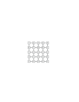
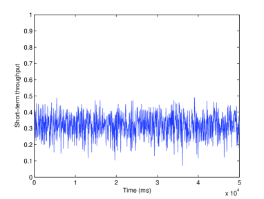
Refer to caption
Figure 13: Conflict graph of a 2-D lattice network
Refer to caption
(a) Tp=25superscript𝑇𝑝25T^{p}=25
Refer to caption
(b) Tp=40superscript𝑇𝑝40T^{p}=40
Refer to caption
(c) Tp=70superscript𝑇𝑝70T^{p}=70
Refer to caption
(d) Tp=100superscript𝑇𝑝100T^{p}=100
Figure 14: Short-term throughput of link 13 in the 2-D lattice network

However, as mentioned before, it remains an open problem to exact characterize the relationship between short-term fairness (in particular the standard deviation of the access delay) and Tpsuperscript𝑇𝑝T^{p} (or equivalently, rmaxsubscript𝑟𝑚𝑎𝑥r_{max}) in general topologies. We are interested to further explore useful methods to quantify the relationship.

References

  • [1] F. P. Kelly, “Reversibility and Stochastic Networks,” Wiley, 1979.
  • [2] S. Boyd and L. Vandenberghe, “Convex Optimization”, Cambridge University Press, 2004.
  • [3] L. Tassiulas and A. Ephremides, “Stability Properties of Constrained Queueing Systems and Scheduling Policies for Maximum Throughput in Multihop Radio Networks,” IEEE Transactions on Automatic Control, vol. 37, no. 12, pp. 1936-1948, Dec. 1992.
  • [4] X. Lin, N.B. Shroff, R. Srikant, “A Tutorial on Cross-Layer Optimization in Wireless Networks,” IEEE Journal on Selected Areas in Communications, 2006.
  • [5] J. M. Harrison and R. J. Williams, “Workload interpretation for Brownian models of stochastic processing networks,” Mathematics of Operations Research, vol. 32, pp. 808-820, 2007.
  • [6] P. Chaporkar, K. Kar, and S. Sarkar, “Throughput guarantees in maximal scheduling in wireless networks,” in the 43rd Annual Allerton Conference on Communication, Control and Computing, Sep. 2005.
  • [7] X. Wu and R. Srikant, “Scheduling Efficiency of Distributed Greedy Scheduling Algorithms in Wireless Networks,” in IEEE INFOCOM 2006, Barcelona, Spain, Apr. 2006.
  • [8] J. Ni and R. Srikant, “Distributed CSMA/CA Algorithms for Achieving Maximum Throughput in Wireless Networks,” in Information Theory and Applications Workshop, Feb. 2009.
  • [9] A. Dimakis and J. Walrand, “Sufficient Conditions for Stability of Longest-Queue-First Scheduling: Second-Order Properties Using Fluid Limits,” Advances in Applied Probability, vol. 38, no. 2, pp. 505–521, 2006.
  • [10] C. Joo, X. Lin, and N. Shroff, “Understanding the Capacity Region of the Greedy Maximal Scheduling Algorithm in Multi-Hop Wireless Networks,” in IEEE INFOCOM 2008, Phoenix, Arizona, Apr. 2008.
  • [11] G. Zussman, A. Brzezinski, and E. Modiano, “Multihop Local Pooling for Distributed Throughput Maximization in Wireless Networks,” in IEEE INFOCOM 2008, Phoenix, Arizona, Apr. 2008.
  • [12] M. Leconte, J. Ni, and R. Srikant, “Improved Bounds on the Throughput Efficiency of Greedy Maximal Scheduling in Wireless Networks,” in ACM MOBIHOC, May 2009.
  • [13] A. Proutiere, Y. Yi, and M. Chiang, “Throughput of Random Access without Message Passing,” in Conference on Information Sciences and Systems, Princeton, NJ, USA, Mar. 2008.
  • [14] R. R. Boorstyn, A. Kershenbaum, B. Maglaris, and V. Sahin, “Throughput Analysis in Multihop CSMA Packet Radio Networks,” IEEE Transactions on Communications, vol. 35, no. 3, pp. 267-274, Mar. 1987.
  • [15] G. Bianchi, “Performance Analysis of the IEEE 802.11 Distributed Coordination Function,” IEEE Journal on Selected Areas in Communications, vol. 18, no. 3, pp. 535-547, 2000.
  • [16] L. Jiang and J. Walrand, “A Distributed CSMA Algorithm for Throughput and Utility Maximization in Wireless Networks,” in the 46th Annual Allerton Conference on Communication, Control, and Computing, Sep. 23-26, 2008.
  • [17] S. Rajagopalan and D. Shah, “Distributed Algorithm and Reversible Network”, in Conference on Information Sciences and Systems, Princeton, NJ, USA, Mar. 2008.
  • [18] P. Marbach, A. Eryilmaz, and A. Ozdaglar, “Achievable Rate Region of CSMA Schedulers in Wireless Networks with Primary Interference Constraints,” in IEEE Conference on Decision and Control, 2007.
  • [19] L. Jiang and S. C. Liew, “Improving Throughput and Fairness by Reducing Exposed and Hidden Nodes in 802.11 Networks,” IEEE Transactions on Mobile Computing, vol. 7, no. 1, pp. 34-49, Jan. 2008.
  • [20] C. Bordenave, D. McDonald, A. Proutiere, “Performance of random medium access control, an asymptotic approach,” in Proceedings of the ACM Sigmetrics 2008, pp. 1-12.
  • [21] F. P. Kelly, “Loss networks,” Ann. Appl. Prob., vol. 1, no. 3, 1991.
  • [22] J. Liu, Y. Yi, A. Proutiere, M. Chiang, and H. V. Poor, “Towards utility optimal random access without message passing,” (Invited Paper) Wiley Journal on Wireless Communications and Mobile Computing, Special Issue on Advances in Wireless Communications and Networking, vol. 10, no. 1, pp. 115-128, Jan. 2010.
  • [23] V. Borkar, “Stochastic Approximation: A Dynamical Systems Viewpoint,” 2008.
  • [24] A. Kumar, E. Altman, D. Miorandi, and M. Goyal, “New insights from a fixed point analysis of single cell IEEE 802.11 WLANs,” In Proc. IEEE INFOCOM, USA, Mar. 2005.
  • [25] X. Wang and K. Kar, “Throughput Modelling and Fairness Issues in CSMA/CA Based Ad-Hoc Networks,” in IEEE INFOCOM 2005, Miami, Florida, Mar. 2005.
  • [26] M. Durvy, O. Dousse and P. Thiran, “On the Fairness of CSMA Networks,” IEEE Journal on Selected Areas in Communications, vol. 27, no. 7, pp. 1093-1104, Sep. 2009.
  • [27] S. C. Liew, C. Kai, J. Leung, and B. Wong, “Back-of-the-Envelope Computation of Throughput Distributions in CSMA Wireless Networks,” in IEEE ICC, 2009.
  • [28] P.M. van de Ven, J.S.H. van Leeuwaarden, T.J.J. Denteneer, A.J.E.M. Janssen, “Spatial fairness in wireless multi-access networks,” in Proc. 4th International Conference on Performance Evaluation Methodologies and Tools (ValueTools’09), Pisa, Italy, Oct. 2009.
  • [29] L. Jiang and J. Walrand, “Approaching Throughput-Optimality in a Distributed CSMA Algorithm: Collisions and Stability,” (invited), ACM Mobihoc’09 S3 Workshop, May 2009.
  • [30] L. Jiang and J. Walrand, “Approaching throughput-optimality in a Distributed CSMA Algorithm with Contention Resolution,” Technical Report, UC berkeley, Mar. 2009. URL: http://www.eecs.berkeley.edu/Pubs/TechRpts/2009/EECS-2009-37.html
  • [31] L. Jiang, D. Shah, J. Shin, J. Walrand, “Distributed Random Access Algorithm: Scheduling and Congestion Control,” http://arxiv.org/abs/0907.1266
  • [32] L. Jiang and J. Walrand, “A Distributed CSMA Algorithm for Throughput and Utility Maximization in Wireless Networks,” Technical Report, UC berkeley, Aug. 2009. http://www.eecs.berkeley.edu/Pubs/TechRpts/2009/EECS-2009-124.html
Libin Jiang received his Ph.D. degree in Electrical Engineering & Computer Sciences from the University of California at Berkeley in 2009. Earlier, he received the B.Eng. degree from the University of Science and Technology of China in 2003, and the M.Phil. degree from the Chinese University of Hong Kong in 2005. His research interests include wireless networks, communications and game theory. He received the David J. Sakrison Memorial Prize in 2010 for outstanding doctoral research, and the best presentation award in the ACM Mobihoc’09 S3 Workshop.
Jean Walrand received his Ph.D. in EECS from UC Berkeley, where he has been a professor since 1982. He is the author of An Introduction to Queueing Networks (Prentice Hall, 1988) and of Communication Networks: A First Course (2nd ed. McGraw-Hill,1998) and co-author of High Performance Communication Networks (2nd ed, Morgan Kaufman, 2000). Prof. Walrand is a Fellow of the Belgian American Education Foundation and of the IEEE and a recipient of the Lanchester Prize and of the Stephen O. Rice Prize.