FFT-LB modeling of thermal liquid-vapor systems

Abstract

We further develop a thermal LB model for multiphase flows. In the improved model, we propose to use the windowed FFT and its inverse to calculate both the convection term and external force term. By using the new scheme, Gibbs oscillations can be damped effectively in unsmooth regions while the high resolution feature of the spectral method can be retained in smooth regions. As a result, spatiotemporal discretization errors are decreased dramatically and the conservation of total energy is much better preserved. A direct consequence of the improvements is that the unphysical spurious velocities at the interfacial regions can be damped to neglectable scale. With the new model, the phase diagram of the liquid-vapor system obtained from simulation is more consistent with that from theoretical calculation. Very sharp interfaces can be achieved. The accuracy of simulation results is also verified by the Laplace law. The high resolution, together with the low complexity of the FFT, endows the proposed method with considerable potential, for studying a wide class of problems in the field of multiphase flows and for solving other partial differential equations.

1 Introduction

During the past two decades, the lattice Boltzmann (LB) method has been developed rapidly and has been successfully applied to various fields [1], ranging from magnetohydrodynamics [2, 3, 4], to flows of suspensions [5, 6], flows through porous media [7, 8], compressible fluid dynamics [9, 10, 11, 12, 13, 14], wave propagation [15, 16], etc. Apart from the fields listed above, this versatile method is particularly promising in the area of multiphase systems [17, 18, 19, 20, 21, 22, 23]. This is partly owing to its intrinsic kinetic nature, which makes the inter-particle interactions (IPI) be incorporated easily and flexibly, and, in fact, the IPI is the underlying microscopic physical reason for phase separation and interfacial tension in multiphase systems.

So far, several LB multiphase models have been proposed. Among them, the four well-known models are the chromodynamic model by Gunstensen et al. [17], the pseudo-potential model by Shan and Chen (SC) [18], the free-energy model by Swift et al. [19], and the HCZ model by He, Chen, and Zhang [20]. The chromodynamic model is developed from the two-component Lattice Gas Automata (LGA) model originally proposed by Rothman and Keller [24]. In this model, the red and blue colored particles are employed to represent two different fluids. Phase separation is achieved through controlling the IPI based on the color gradient. Similar to the treatment in molecular dynamics (MD), in SC model, non-local interactions between particles at neighboring lattice sites are incorporated. The interactions determine the form of the equation of state (EOS). Phase separation or mixing is governed by the mechanical instability when the sign of the IPI is properly chosen. In the free-energy model, besides the mass and momentum conservation constraints, additional ones are imposed on the equilibrium distribution function, which makes the pressure tensor consistent with that of the free-energy functional of inhomogeneous fluids. In the HCZ model, two distribution functions are used. The first one is used to compute the pressure and the velocity fields. The other one is used to track interfaces between different phases. Molecular interactions, such as the molecular exclusion volume effect and the intermolecular attraction, are incorporated to simulate phase separation and interfacial dynamics.

The aforementioned models have been successfully applied to a wide variety of multiphase and/or multicomponent flow problems, including drop breakup [25, 26], drop collisions [27], wetting [28, 29], contact line motion [30, 31], chemically reactive fluids [32], phase separation and phase ordering phenomena [19, 21, 23, 33], hydrodynamic instability [34, 35], etc. However, despite this, the current LB versions for multiphase flows are still subjected to, at least, one of the following constrains (i) the isothermal constraint (i.e., the deficiency of temperature dynamic), (ii) the limited density ratio and temperature range, (iii) the spurious velocities. This paper addresses mainly the last restriction and the total energy conservation in practical simulations.

Spurious velocities extensively exist in simulations of the liquid-vapor system and reach their maxima at the interfacial regions, indicating deviation from the real physics of a fluid system. Reducing and eliminating the unphysical velocities are of great importance to the simulations of multiphase flows. Firstly, large spurious velocities will lead to numerical instability. Secondly, the local velocities are small during phase separation and coarsening. If the spurious currents are too large, then we may not be able to separate the spurious currents from the real local flows, which is especially true in the case of phase separation with high viscosity. Thirdly, for a thermal multiphase system, accurate flow velocities are required in order to obtain an accurate temperature field [36].

In dealing with this issue, extensive efforts have been made during the past years. Wagner [37] pointed out that the origin of the spurious currents is due to the incompatibility between the discretizations of driving forces for the order parameter and momentum equation. Therefore, he suggested to cure the spurious velocities by removing the nonideal terms from the pressure tensor and introducing them as a body force. Sofonea and Cristea et al. [23, 38] presented a finite difference LB (FDLB) approach and proposed two ways to eliminate the unwanted currents. In the first way, a high-accuracy numerical scheme, the flux limiter method is employed to calculate the convection term of the LB equation. In the second way, a correction force term is introduced to the LB equation that cancels the spurious velocities and allows to recover the mass equation correctly. Shan [39] and Succi et al. [22] showed that the origin of the spurious currents are due to the insufficient isotropy in the calculation of density gradient. Therefore, using the information of the density field on an extended neighboring $\mathbf{x}+\mathbf{e}_{i}$ of a given site to construct high order isotropic difference operators, is the key for the correct discretization of spatial derivatives and taming the spurious currents in the interface. Yuan et al. [36] demonstrated that smaller parasitical velocities and higher density ratio can be achieved using more realistic EOS in a single-component multiphase LB model. Lee and Fischer [40] reported that the use of the potential form of the surface tension and the isotropic FD scheme can eliminate parasitic currents to round-off. Seta and Okui [41] composed a more accurate fourth order scheme to calculate the derivatives in the pressure tensor. This convenient approach reduces the amplitude of spurious velocities to about one half of that from the second order scheme. Pooley and Furtado [42] analyzed the causes of spurious velocities in a free-energy LB model and provided two improvements. First, by making a suitable choice of the equilibrium distribution and using the nine-point stencils (NPS) scheme to calculate derivatives, the magnitude of spurious velocities can be decreased by an order. Moreover, a momentum conserving force is presented to further reduce the spurious velocities. Yeomans et al. [43] identified two sources of the spurious velocities, the long range effects and the bounce-back boundary conditions, when a single relaxation time (SRT) LB algorithm is used to solve the hydrodynamic equations of a binary fluids. Aiming to reduce the unwanted velocities, they proposed a revised LB method based on a multiple-relaxation-time (MRT) algorithm.

In this work, we present a thermal LB model for simulating thermal liquid-vapor system with neglectable spurious velocities. This model is a further development of the one originally proposed by Watari and Tsutahara (WT) [9] and then developed by Gonnella, Lamura and Sofonea (GLS) [44]. The original WT model works only for ideal gas. GLS introduced an appropriate IPI force term to describe van der Waals (VDW) fluids. Here we introduce a windowed FFT (WFFT) scheme to calculate the convection term and the force term. The improved model is convenient to compromise the high accuracy and stability. With the new model, non-conservation problem of total energy due to spatiotemporal discretizations is much better controlled and spurious currents in equilibrium interfaces are significantly damped.

The rest of the paper is structured as follows. In the next section the thermal LB models for ideal gas and for VDW fluids are briefly reviewed. In section III we illustrate the necessity of the further development and detail the usage of the WFFT scheme and its inverse. Comparisons and analysis of numerical results from different schemes are presented in section IV, where we will show how the spurious velocities around linear and curved interfaces can be reduced by the new model. Finally, in section V, we summarize the results and suggest directions for future research.

2 The model

2.1 Original WT model for ideal gas system

The thermal multiphase model is developed from the thermal LB model, originally, proposed by WT, which is based on a multispeed approach. In this approach, additional speeds are required and higher order velocity terms are included in the equilibrium distribution function to obtain the macroscopic temperature field.

WT model uses the following discrete-velocity-model (DVM) which involves a set of 33 nondimensionalized velocities

$$\mathbf{v}_{0}=0\text{, }\mathbf{v}_{ki}=v_{k}[\cos(\frac{i-1}{4}\pi)\text{,}\sin(\frac{i-1}{4}\pi)]\text{,}$$ (1)

where subscript $k=1$,…,$4$ indicates the $k$-th group of the particle velocities whose speed is $v_{k}$ and $i=1$,…,$8$ indicates the direction of particle’s speed. In our simulations we set $\mathrm{\ }v_{1}=1.00$,$\mathrm{\ }v_{2}=1.90$,$\mathrm{\ }v_{3}=2.90$, and $\mathrm{\ }v_{4}=4.30$.

The distribution function $f_{ki}$, discrete in space and time, evolves according to a SRT Boltzmann equation

$$\frac{\partial f_{ki}}{\partial t}+\mathbf{v}_{ki}\cdot\frac{\partial f_{ki}}{\partial\mathbf{r}}=-\frac{1}{\tau}\left[f_{ki}-f_{ki}^{eq}\right]\text{,}$$ (2)

where $f_{ki}^{eq}$, $\mathbf{r}$, and $\tau$ denote the local equilibrium distribution function, the spatial coordinate, and the relaxation time, respectively. $f_{ki}^{eq}$ is expressed as a series expansion in the local velocity

$$f_{ki}^{eq} = \frac{\rho}{{2\pi T}}\exp(-\frac{{v_{ki}^{2}}}{{2T}})\exp(-\frac{{u^{2}-2uv_{ki}}}{{2T}})$$ (3)

$$= \rho F_{k}[(1-\frac{{u^{2}}}{{2T}}+\frac{{u^{4}}}{{8T^{2}}})+\frac{{v_{ki\varepsilon}u_{\varepsilon}}}{T}(1-\frac{{u^{2}}}{{2T}})$$

$$+\frac{{v_{ki\varepsilon}v_{ki\pi}u_{\varepsilon}u_{\pi}}}{{2T^{2}}}(1-\frac{{u^{2}}}{{2T}})+\frac{{v_{ki\varepsilon}v_{ki\pi}v_{ki\eta}u_{\varepsilon}u_{\pi}u_{\eta}}}{{6T^{3}}}$$

$$+\frac{{v_{ki\varepsilon}v_{ki\pi}v_{ki\eta}v_{ki\lambda}u_{\varepsilon}u_{\pi}u_{\eta}u_{\lambda}}}{{24T^{4}}}]+\cdot\cdot\cdot\text{,}$$

where the weight factors are

$$F_{k} = \frac{{1}}{{v_{k}^{{2}}(v_{k}^{{2}}-v_{k+1}^{{2}})(v_{k}^{{2}}-v_{k+2}^{{2}})(v_{k}^{{2}}-v_{k{+3}}^{{2}})}}{[48}T^{{4}}-{6(}v_{k+1}^{2}{+}v_{k+2}^{{2}}{+}v_{k+3}^{{2}}{)}T^{{3}}$$ (4)

$$+{(}v_{k+1}^{{2}}v_{k+2}^{{2}}{+}v_{k+2}^{{2}}v_{k+3}^{{2}}{+}v_{k+3}^{{2}}v_{k+1}^{{2}}{)}T^{{2}}-\frac{{v_{k+1}^{{2}}v_{k+2}^{{2}}v_{k+3}^{{2}}}}{{4}}T{]}\text{{,}}$$

$$F_{0}={1}-{8(}F_{1}{+}F_{2}{+}F_{3}{+}F_{4}{)}\text{,}$$ (5)

with

$$\left\{{k+l}\right\}=\left\{\begin{array}[]{cc}k+l\text{,}&k+l\leq 4\text{;}\\ k+l-4\text{,}&k+l>4\text{;}\end{array}l\in\{1,2,3\}\text{.}\right.$$ (6)

Hydrodynamic quantities, such as density, velocity, and temperature are determined from the following moments

$$\rho=\sum_{ki}f_{ki}^{eq}\text{,}$$ (7)

$$\rho\mathbf{u}=\sum_{ki}\mathbf{v}_{ki}f_{ki}^{eq}\text{,}$$ (8)

$$\rho T=\sum_{ki}\frac{1}{2}(\mathbf{v}_{ki}-\mathbf{u})^{2}f_{ki}^{eq}\text{.}$$ (9)

The combination of the above DVM and the general FD scheme with first-order forward in time and second-order upwinding in space composes the original FDLB model by WT. In the FDLB model, particle velocities are independent from the lattice configuration. As a result, higher-order numerical schemes can be used to reduce the numerical viscosity and to enhance the stability of the model. This is of great importance to LB simulations, especially in phase separation studies, where long lasting simulations are needed to establish the growth properties.

2.2 GLS model for multiphase system

WT model can be applied to compressible flows with small Mach number and the revised version [13] extends it to compressible flows with high Mach number due to better numerical stability. Nevertheless, neither the original one nor the improved one has the ability to describe multiphase flows, since both models lead to the ideal EOS only, which do not support thermodynamical two-phase state.

Fortunately, by incorporating a forcing term, the improved model can be applied to thermal liquid-vapor systems. Compared to isothermal models, the variable temperature that the GLS model can be implemented is of great importance, since thermal effects are ubiquitous and sometimes dominant in an important class of flows [45]. Examples are referred to boiling [46], distillation, as well as the dynamics of phase separation [47, 48], where the freedom in temperature limits the rate of phase separation and induces different rheological and morphological behaviors. Dynamic effects of temperature can not be considered in isothermal models, therefore, most studies have been restricted to either isothermal systems or the systems where effects of temperature dynamics are negligible.

The forcing term introduced by GLS is added into the right-hand side (RHS) of Eq. (2)

$$\frac{\partial f_{ki}}{\partial t}+\mathbf{v}_{ki}\cdot\frac{\partial f_{ki}}{\partial\mathbf{r}}=-\frac{1}{\tau}\left[f_{ki}-f_{ki}^{eq}\right]+I_{ki}\text{,}$$ (10)

where $I_{ki}$ takes the following form,

$$I_{ki}=-[A+B_{\alpha}(v_{ki\alpha}-u_{\alpha})+(C+C_{q})(v_{ki\alpha}-u_{\alpha})^{2}]f_{ki}^{eq}\text{.}$$ (11)

$I_{ki}$ in Eq. (10) is introduced to control the equilibrium properties of the liquid-vapor systems and allows to recover the following equations for VDW fluids [44],

$$\partial_{t}\rho+\partial_{\alpha}(\rho u_{\alpha})=0\text{,}$$ (12)

$$\partial_{t}(\rho u_{\alpha})+\partial_{\beta}(\rho u_{\alpha}u_{\beta}+\Pi_{\alpha\beta}-\sigma_{\alpha\beta})=0\text{,}$$ (13)

$$\partial_{t}e_{T}+\partial_{\alpha}[e_{T}u_{\alpha}+(\Pi_{\alpha\beta}-\sigma_{\alpha\beta})u_{\beta}-\kappa_{T}\partial_{\alpha}T]=0\text{,}$$ (14)

where

$$\Pi_{\alpha\beta}=P^{w}\delta_{\alpha\beta}+\Lambda_{\alpha\beta}\text{,}$$ (15)

$$\sigma_{\alpha\beta}=\eta(\partial_{\alpha}u_{\beta}+\partial_{\beta}u_{\alpha}-\partial_{\gamma}u_{\gamma}\delta_{\alpha\beta})+\zeta\partial_{\gamma}u_{\gamma}\delta_{\alpha\beta}\text{,}$$ (16)

and

$$e_{T}=\rho T-9\rho^{2}/8+K\left|\nabla\rho\right|^{2}/2+\rho u^{2}/2\text{,}$$ (17)

represent the non-viscous stress, the dissipative tensor, and the total energy density, respectively. $\kappa_{T}$, $\eta$, and $\zeta$ are heat conductivity, shear, and bulk viscosities. $P^{w}$ and $\Lambda_{\alpha\beta}$ in Eq. (15) are the VDW EOS and the contribution of density gradient to pressure tensor, which have the following expressions

$$P^{w}=3\rho T/(3-\rho)-9\rho^{2}/8\text{,}$$ (18)

$$\Lambda_{\alpha\beta}=M\partial_{\alpha}\rho\partial_{\beta}\rho-[\rho T\partial_{\gamma}\rho\partial_{\gamma}(M/T)]\delta_{\alpha\beta}-M(\rho\nabla^{2}\rho+\left|\nabla\rho\right|^{2}/2)\delta_{\alpha\beta}\text{.}$$ (19)

The expression $M=K+HT$ allows a dependence of the surface tension on temperature, where $K$ is the surface tension coefficient and $H$ is a constant.

In order to recover Eqs. (12)-(14), five constraints are imposed on the forcing term, which make coefficients in Eq. (11) as the following form

$$A=-2(C+C_{q})T\text{,}$$ (20)

$$B_{\alpha}=\frac{1}{\rho T}[\partial_{\alpha}(P^{w}-\rho T)+\partial_{\beta}\Lambda_{\alpha\beta}-\partial_{\alpha}(\zeta\partial_{\gamma}u_{\gamma})]\text{,}$$ (21)

$$C = \frac{1}{2\rho T^{2}}\{(P^{w}-\rho T)\partial_{\gamma}u_{\gamma}+\Lambda_{\alpha\beta}\partial_{\alpha}u_{\beta}-(\zeta\partial_{\gamma}u_{\gamma})\partial_{\alpha}u_{\alpha}$$ (22)

$$+\frac{9}{8}\rho^{2}\partial_{\gamma}u_{\gamma}+K[-\frac{1}{2}(\partial_{\gamma}\rho)(\partial_{\gamma}\rho)(\partial_{\alpha}u_{\alpha})$$

$$-\rho(\partial_{\gamma}\rho)(\partial_{\gamma}\partial_{\alpha}u_{\alpha})-(\partial_{\gamma}\rho)(\partial_{\gamma}u_{\alpha})(\partial_{\alpha}\rho)]\}\text{,}$$

$$C_{q}=\frac{1}{2\rho T^{2}}\partial_{\alpha}[2q\rho T(\partial_{\alpha}T)]\text{.}$$ (23)

It is worth noting that in this model the Prandtl number $\Pr=\eta/\kappa_{T}=\tau/2(\tau-q)$ can be changed by adjusting the parameter $q$ in the term $C_{q}$.

3 Thermal LB model based on the WFFT approach

In this section, we present our contribution to the thermal multiphase LB model: spatial derivatives in the convection term $\mathbf{v}_{ki}\cdot\partial f_{ki}/\partial\mathbf{r}$ and in the forcing term $I_{ki}$, are calculated via the WFFT algorithm and its inverse.

To illustrate the necessity, we present simulation results for a thermal phase separation process by various numerical schemes. Here the time derivative is calculated using the first-order forward Euler FD scheme. The spatial derivatives in $I_{ki}$ are calculated using the second-order central difference scheme. Spatial derivatives in the convection term $\mathbf{v}_{ki}\cdot\partial f_{ki}/\partial\mathbf{r}$ are calculated using various schemes listed as follows:

3.1 second-order central difference scheme

Let $J-1$, $J$ and $J+1$ be three successive nodes of the one dimensional lattice. Using the second-order central difference scheme to discretize the convention term, Eq. (10) can be rewritten in a conservative form

$$f_{ki,J}^{n+1}=f_{ki,J}^{n}-\frac{{c_{ki\alpha}}}{2}(f_{ki,J+1}^{n}-f_{ki,J-1}^{n})-\frac{{\Delta t}}{\tau}(f_{ki,J}^{n}-f_{ki,J}^{eq,n})+I_{ki,J}^{n}\Delta t\text{,}$$ (24)

where ${\Delta t}$ and ${c_{ki\alpha}=v}_{ki\alpha}\Delta t/\Delta r_{\alpha}{\ }$are the time step and the Courant-Friedrichs-Levy (CFL) number.

3.2 Lax-Wendroff (LW) scheme

Compared with the second-order central difference scheme, the LW scheme contributes a dissipation term, which is in favor of the numerical stability. Then, by using this scheme, Eq. (10) can be formulated as

$$f_{ki,J}^{n+1} = f_{ki,J}^{n}-\frac{{c_{ki\alpha}}}{2}(f_{ki,J+1}^{n}-f_{ki,J-1}^{n})+\frac{{c_{ki\alpha}^{2}}}{2}(f_{ki,J+1}^{n}-2f_{ki,J}^{n}+f_{ki,J-1}^{n})$$ (25)

$$-\frac{{\Delta t}}{\tau}(f_{ki,J}^{n}-f_{ki,J}^{eq,n})+I_{ki,J}^{n}\Delta t\text{.}$$

3.3 Modified-LW (MLW) scheme

As we know, the LW scheme is very dissipative and has a strong “ smoothing effect". Obviously, it is not favorable to recover the sharp interface in the multiphase system. To further improve the numerical accuracy, the modified partial differential equation (MPDE) remainder after discretizing with Eq. (25) is derived [49]

$$R=-\frac{{v_{ki\alpha}(1-c_{ki\alpha}^{2})}}{6}\Delta r_{\alpha}^{2}\frac{{\partial^{3}f}}{{\partial r^{3}}}-\frac{{v_{ki\alpha}c_{ki\alpha}(1-c_{ki\alpha}^{2})}}{8}\Delta r_{\alpha}^{3}\frac{{\partial^{4}f}}{{\partial r^{4}}}+\cdots\text{.}$$ (26)

It is clear that the first and the second terms in the RHS of Eq. (26) correspond to the third-order dispersion error $R_{3}$ and the fourth-order dissipation error $R_{4}$, respectively. Therefore, we can add the dispersion term into the RHS of Eq. (10) to compensate the dispersion error

$$\frac{{\partial f_{ki}}}{{\partial t}}+\mathbf{v}_{ki}.\frac{\partial}{{\partial\mathbf{r}}}f_{ki} = -\frac{{1}}{\tau}(f_{ki}-f_{ki}^{eq})+I_{ki}$$ (27)

$${+}\frac{{v_{ki\alpha}(1-c_{ki\alpha}^{2})}}{6}\Delta r_{\alpha}^{2}\frac{{\partial^{3}f}}{{\partial r^{3}}}\text{.}$$

Furthermore, we can add the dissipation term into RHS of Eq. (27). Using the 2nd-CD scheme to discrete $R_{3}$ and $R_{4}$ gives

$$\bar{R}_{3}=\frac{{c_{ki\alpha}(1-c_{ki\alpha}^{2})}}{{12}}(f_{ki,J+2}^{n}-2f_{ki,J+1}^{n}+2f_{ki,J-1}^{n}-f_{ki,J-2}^{n})\text{,}$$ (28)

and

$$\bar{R}_{4}=\frac{{c_{ki\alpha}^{2}(1-c_{ki\alpha}^{2})}}{8}(f_{ki,J+2}^{n}-4f_{ki,J+1}^{n}+6f_{ki,J}^{n}-4f_{ki,J-1}^{n}+f_{ki,J-2}^{n})\text{.}$$ (29)

The bars above $R_{3}$ and $R_{4}$ indicate that they are discretized. If only $\bar{R}_{3}$ is added into the RHS of Eq. (25), for convenience of description, we refer to this scheme as MLW1. If both $\bar{R}_{3}$ and $\bar{R}_{4}$ are added into the RHS of Eq. (25), then a more accurate LB equation is obtained, and we refer to this scheme as MLW2.

3.4 Flux limiter (FL) scheme

Figure 1: (Color online) Characteristic line on the square lattice for the direction $i=2$.

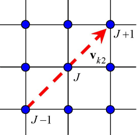
The FL scheme has been widely employed by Sofonea et al. [23, 38] to reduce the spurious velocities and to improve the numerical stability in liquid-vapor systems. Figure 1 shows the characteristic line on the square LB lattice for direction $i=2.$ When using this approach to compute the convective term along the characteristic line, Eq. (10) becomes

$$f_{ki,J}^{n+1} = f_{ki,J}^{n}-\frac{{v_{k}\Delta t}}{{A_{i}\Delta r_{\alpha}}}[F_{ki,J+1/2}^{n}-F_{ki,J-1/2}^{n}]$$ (31)

$$-\frac{{1}}{\tau}(f_{ki,J}^{n}-f_{ki,J}^{n,{eq}})\Delta t+I_{ki,J}^{n}\Delta t\text{,}$$

with

$$A_{i}=\left\{\begin{array}[]{cc}1\text{,}&i\in\{1,3,5,7\}\text{;}\\ \sqrt{2}\text{,}&i\in\{2,4,6,8\}\text{.}\end{array}\right.$$ (32)

$F_{ki,J+1/2}^{n}$ and $F_{ki,J-1/2}^{n}$ in Eq. (31) are two fluxes, which are defined as

$$F_{ki,J+1/2}^{n}=f_{ki,J}^{n}+\frac{1}{2}(1-\frac{{v_{k}\Delta t}}{{A_{i}\Delta r_{\alpha}}})[f_{ki,J+1}^{n}-f_{ki,J}^{n}]\psi(\theta_{ki,J}^{n})\text{,}$$ (33)

$$F_{ki,J-1/2}^{n}=F_{ki,(J-1)+1/2}^{n}\text{,}$$ (34)

where the flux limiter $\psi(\theta_{ki,J}^{n})$ is expressed as a smooth function

$$\theta_{ki,J}^{n}=\frac{f_{ki,J}^{n}-f_{ki,J-1}^{n}}{f_{ki,J+1}^{n}-f_{ki,J}^{n}}\text{.}$$ (35)

In particular, if $\psi(\theta_{ki,J}^{n})=0$, it corresponds to the first-order upwind scheme and $\psi(\theta_{ki,J}^{n})=1$ to the LW scheme. A wide choice of flux limiters can work well with LB models. In this work, we will use the monitorized central difference (MCD) FL, which is most widely used by Sofonea et al.

$$\psi(\theta_{ki,J}^{n})=\left\{\begin{array}[]{cc}0\text{,}&\theta_{ki,J}^{n}\leq 0\text{,}\\ 2\theta_{ki,J}^{n}\text{,}&0<\theta_{ki,J}^{n}\leq 1/3\text{,}\\ (1+\theta_{ki,J}^{n})/2\text{,}&1/3<\theta_{ki,J}^{n}\leq 3\text{,}\\ 2\text{,}&3<\theta_{ki,J}^{n}\text{.}\end{array}\right.$$ (36)

3.5 NPS scheme

Recently, a new scheme, named the NPS scheme, has been widely used to calculate the spatial derivatives by many scholars so as to ensure higher isotropy and to reduce spurious velocities [36, 42, 43, 50, 51]. The general choice of stencils for calculating the derivatives and the laplacian are

$$\bar{\partial}_{x} = \frac{1}{{\Delta x}}\left[\begin{array}[]{ccc}-B&0&B\\ -A&0&A\\ -B&0&B\end{array}\right]$$ (40)

$$= \partial_{x}+\frac{1}{6}\Delta x^{2}\partial_{x}^{3}+2B\Delta x^{2}\partial_{x}\partial_{y}^{2}+\cdots\text{,}$$ (41)

and

$$\bar{\nabla}^{2} = \frac{1}{{\Delta x^{2}}}\left[\begin{array}[]{ccc}F&E&F\\ E&-4(E+F)&E\\ F&E&F\end{array}\right]$$ (45)

$$= \nabla^{2}+\frac{{\Delta x^{2}}}{{12}}(\partial_{x}^{4}+\partial_{y}^{4})+F\Delta x^{2}\partial_{x}^{2}\partial_{y}^{2}+\cdots\text{,}$$ (46)

with $2A+4B=1$ and $E+2F=1$ to keep consistency between the continuous and discrete operators. The bars above $\partial_{x}$ and $\nabla^{2}$ represent that they are discrete operators. The central entry denotes the lattice node at which the derivative is calculated, and the remaining entries are the eight neighbor nodes around the central one. $B$ and $F$ are two free parameters that are chosen to minimize the spurious velocities. A large amount of numerical tests indicate that the best choice is $B=1/12$ and $F=1/6$ in the GLS model. In our simulations, both the convection term and the forcing term are calculated by this way.

Figure 2: (Color online) Variations of total energy $\Delta e_{T}(t)=e_{T}(t)-e_{T}(0)$ for a phase separating process with various numerical schemes.

Next, we conduct simulations of a thermal phase separation process with numerical schemes listed above. Initial conditions of our test are chosen as

$$(\rho\text{, }T\text{, }u\text{, }v)=(1+\Delta\text{,}0.85\text{, }0.0\text{, }0.0)\text{,}$$ (47)

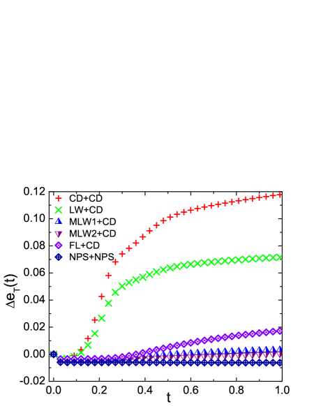
where $\Delta$ is a random density with an amplitude $0.001$ and can be regarded as incipient nuclei in the density field. Periodical boundary conditions (PBC) are imposed on a square lattice with $N_{x}=N_{y}=128$. Unless otherwise stated, the remaining parameters are $\Delta x=\Delta y=1/256$, $\Delta t=10^{-5}$, $\tau=10^{-2}$, $K=10^{-5}$, $H=0$, $\zeta=0$, $q=-0.004$, throughout our simulations. Figure 2 shows the variations of total energy $\Delta e_{T}(t)=e_{T}(t)-e_{T}(0)$ for the phase separating process with various numerical schemes. The legend in each case is composed of two parts, ‘A’+‘B’, where ‘A’ is ‘CD’, ‘LW’, ‘MLW1’, ‘MLW2’, ‘FL’ and ‘NPS’ and it shows the scheme to calculate the convection term; ‘B’ is ‘CD’ and ‘NPS’ and it shows the scheme to calculate the forcing term. Figure 2 demonstrates that the total energy density $e_{T}(t)$ is not conservative in simulations even though it is in theoretical analysis. Further survey of these results indicates that the derivation $\Delta e_{T}(t)$ decreases by increasing the accuracy of scheme. Therefore, we conclude that the non-conservation of total energy is mainly due to the spatial discretization errors.

3.6 The WFFT approach

To overcome the problem of energy non-conservation, a new algorithm based on WFFT is proposed. This approach is especially powerful for periodic system and also provides spatial spectral information on hydrodynamic quantities. Moreover, with this approach, higher-order derivatives and fractional-order derivatives can be computed in a convenient way.

For the sake of clarity, we start with the definition of Fourier transform of $f(x_{j})$

$$\widetilde{f}(k)=\Delta x\sum_{j=0}^{N-1}f(x_{j})e^{-\mathbf{i}kx_{j}}\text{,}$$ (48)

and its inverse

$$f(x_{j})=\frac{1}{L}\sum_{n=-N/2}^{N/2-1}\widetilde{f}(k)e^{\mathbf{i}kx_{j}}\text{,}$$ (49)

where $k$ is the module of wave vector $\mathbf{k}$, $\mathbf{i}$ is the imaginary unit, and $\widetilde{f}(k)$ stands for the Fourier transform of a spatial function $f(x)$. In Eq. (49), $k\mathbf{=}2\pi n/L$, and $L=N\Delta x$ is the length of the system divided into $N$ equal segments. The above two equations are exactly correct when $N$ is infinitely large or $\Delta x$ is infinitely small. A general theorem of derivative based on FFT states that [52, 53, 54]

$$\widetilde{f^{\prime}}(k)=\mathbf{i}k\times\widetilde{f}(k)\text{,}$$ (50)

where $\widetilde{f^{\prime}}(k)$ is the Fourier transform of $f^{\prime}(x)$. The theorem suggests a way to calculate spatial derivative $f^{\prime}(x)$, as shown in Fig. 3. Firstly, transform $f(x)$ in real space into $\widetilde{f}(k)$ in reciprocal space; then, multiply $\widetilde{f}(k)$ with $\mathbf{i}k$; finally, take the inverse Fourier transform (IFT) of $\widetilde{f^{\prime}}(k)$, the spatial derivative $f^{\prime}(x)$ can be obtained.

Figure 3: A possible flow chart for differential operator using the FFT scheme and its inverse (IFFT).

The approach mentioned above has excellent accuracy properties, typically well beyond that of standard discretization schemes. In principle, it gives the exact derivative with infinite order accuracy if the function is infinitely differentiable [53, 54, 55, 56], which is another advantage of FFT scheme compared to the FD scheme. In our manuscript, using this virtue, the FFT scheme is designed to approximate the true spatial derivatives, as a result, to eliminate spurious velocities and to guarantee energy conservation.

However, the trouble in proceeding in this manner is that, in many cases, it is difficult to ensure that infinite differentiability condition is satisfied. For example, the Sod shock tube problem [57] contains the shock wave, the rarefaction wave and the contact discontinuity. Then the derivative of hydrodynamic quantity, $\rho^{\prime}(x)$ or $T^{\prime}(x)$ has a discontinuity as the same character as the square wave (see Fig.6 for more details). Then the discontinuity will induce oscillations, known as the Gibbs phenomenon. The Gibbs phenomenon influences the accuracy of the FFT not only in the neighborhood of the point of singularity, but also over the entire computational domain. More importantly, sometimes, it will cause numerical instability. For example, for the problems shown in Figs. 9 and 17 (in Sec. IV), the above approach is unstable due to the Gibbs phenomenon. Recently, there is a trend to use smoothing procedures which attenuate higher-order Fourier coefficients to avoid or at least to reduce these oscillations (i.e., WFFT method) [53, 55, 58, 59]. A straightforward and convenient way to attenuate the higher-order Fourier coefficients is to multiply each Fourier coefficients by a smoothing factor (filter) $\sigma_{k}$, such as the Lanzos filter, raised cosine filter, sharpened raised cosine filter and exponential cutoff filter, as listed in Refs. [53, 58, 59].

In the present study, based on Taylor series expansion of wave number $k$, we present a way to construct smoothing factors. Firstly, we expand $k$ in Taylor series

$$k = \frac{\arcsin[\sin(k\Delta x/2)]}{\Delta x/2}$$ (51)

$$= \frac{1}{\Delta x/2}[\sin(k\Delta x/2)+\frac{1}{6}\sin^{3}(k\Delta x/2)+\frac{3}{40}\sin^{5}(k\Delta x/2)+\frac{5}{112}\sin^{7}(k\Delta x/2)+...]$$

$$= \frac{1}{\Delta x/2}\sum_{n=0}^{\infty}\frac{\Gamma(n/2)\delta_{0,\Theta(n)}\varepsilon(-1+n)}{\sqrt{\pi}n\Gamma(\frac{n+1}{2})}\sin^{n}(k\Delta x/2)\text{,}$$

where $\Gamma(n)=\int_{0}^{\infty}t^{n-1}e^{-t}dt$ is the Gamma function, $\Theta(n)=Mod[-1+n,2]$ is the Mod function, and $\varepsilon(-1+n)$ is the unit step function. Thus, in order to damp the Gibbs oscillations, or in order to filter out more high frequency waves, $k$ may take the form of an appropriately truncated Taylor series expansion of sin$(k\Delta x/2)$. For example, $k$ may take the following forms

$$k_{1}\mathbf{=}\frac{\sin(k\Delta x/2)}{\Delta x/2}\text{,}$$ (52)

$$k_{2}\mathbf{=}k_{1}+\frac{\sin^{3}(k\Delta x/2)/6}{\Delta x/2}\text{,}$$ (53)

$$k_{3}\mathbf{=}k_{2}+\frac{3\sin^{5}(k\Delta x/2)/40}{\Delta x/2}\text{,}$$ (54)

and

$$k_{4}\mathbf{=}k_{3}+\frac{5\sin^{7}(k\Delta x/2)/112}{\Delta x/2}\text{,}$$ (55)

where $k_{1}$ is consistent with the one used in Ref. [60]. Some simple derivations indicate that the above approach with $k_{1}$, $k_{2}$, $k_{3}$, and $k_{4}$ has a second-order, fourth-order, sixth-order, and eighth-order accuracy in space, respectively (see Appendix for more details).

Figure 4: Smoothing factors $\sigma_{k}$ for $k_{1}$, $k_{2}$, $k_{3}$, and $k_{4}$ with $N=128$.

Figure 5: (Color online) Absolute errors for the computed first-order derivative of the test function $f(x)=sin(x)$ with the WFFT algorithm.

Figure 6: (Color online) Comparisons between LB results and exact ones for the one-dimensional modified Sod problem at $t=0.2$. The simulation results (circles) are from the WT model with the WFFT scheme, where the lower-order filter $k_{1}$ is used.

Figure 7: (Color online) Temperature profiles for the modified Sod shock problem obtained from the WFFT schemes with $k$, $k_{1}$, $k_{2}$, $k_{3}$, and $k_{4}$ in (a). The portion in square of (a) is enlarged in (b) for a closing view.

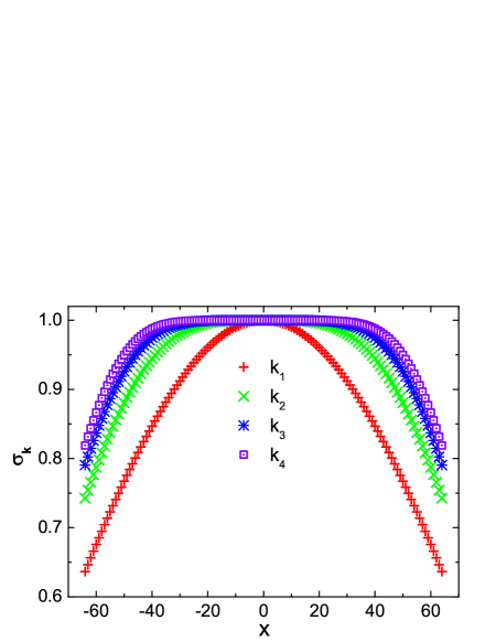
Therefore, smoothing factor for $k_{1}$ takes the following form

$$\sigma_{1}=\frac{k_{1}}{k}=\frac{\sin(n\pi/N)}{n\pi/N}\text{, }n=-N/2\text{,}...\text{,}N/2\text{.}$$ (56)

Smoothing factors $\sigma_{k}$ for $k_{2}$, $k_{3}$, and $k_{4}$ can be calculated in a similar way and are represented in Fig. 4. It is clear that the lower-order smoothing factors $k_{1}$ and $k_{2}$, filter out more high frequency waves, and may result in excessively smeared approximations, which are unfaithful representations of the truth physics. On the other hand, the higher-order smoothing factors $k_{3}$ and $k_{4}$, reserve more higher frequency waves, but may not damp the Gibbs phenomenon (see Fig. 7 for more details), then cause numerical instability. The smoothing factors should survive the dilemma of stability versus accuracy. In other words, they should be minimal but make the evolution stable at the same time.

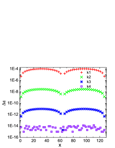
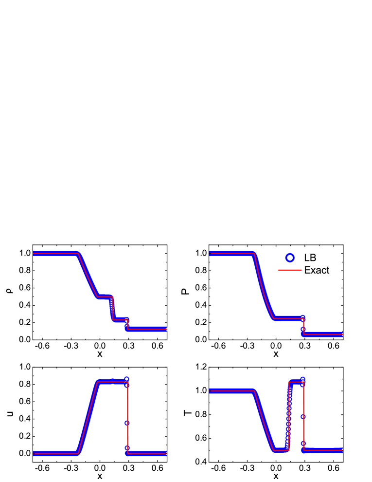
As a simple test, using the WFFT algorithm, the derivative of a infinite differentiable function $f(x)=sin(x)$, is calculated with $k_{1}$, $k_{2}$, $k_{3}$, $k_{4}$, and plotted in Fig. 5. It is clearly seen that when $k_{4}$ is used, the errors reduce to round-off. As another test, the validity of the WFFT scheme is verified by the modified Sod shock tube with higher pressure ratio. For the problem considered, the initial condition is described by

$$\left\{\begin{array}[]{l}\left.{(\rho}\text{{, }}{u}\text{{, }}{v}\text{{, }}{T)}\right|_{L}=(1.0\text{, }0.0\text{, }0.0\text{, }1.0)\text{{,} \ \ \ }x\leq 0\text{;}\\ \left.{(\rho}\text{{, }}{u}\text{{, }}{v}\text{{, }}{T)}\right|_{R}=(0.125\text{, }0.0\text{, }0.0\text{, }0.5)\text{, \ }x>0\text{.}\end{array}\right.$$ (57)

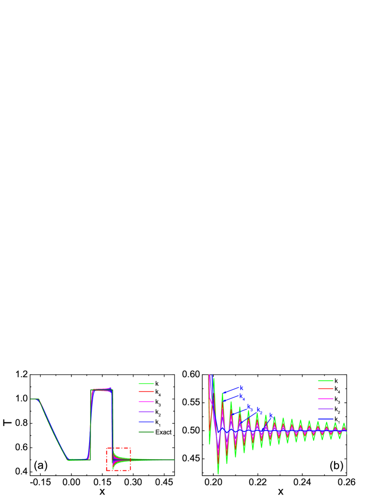
Subscripts “$L$" and “$R$" indicate macroscopic variables at the left and right sides of the discontinuity. The size of grid is $\Delta x=\Delta y=2.5\times 10^{-3}$, time step is $\Delta t=10^{-5}$, and relaxation time is $\tau=3\times 10^{-4}$. Figure 6 shows the computed density, pressure, velocity, and temperature profiles at $t=0.2$, where the circles are for simulation results and solid lines are for analytical solutions. The two sets of results have a satisfying agreement. Figure 7 shows the temperature profiles obtained from the WFFT schemes with $k$, $k_{1}$, $k_{2}$, $k_{3}$, and $k_{4}$ in (a) and local details of the part near the shock wave in (b). One can see that higher-order filters, such as $k_{3}$ and $k_{4}$, have higher accuracy in smooth regions, but cannot refrain the Gibbs phenomenon in unsmooth regions effectively. The lower-order filters, although are too dissipative, can damp the spurious oscillations to neglectable scale, which are capable of shock capturing. Therefore, it should be noted that, for flows without shock waves and/or discontinuities, the WFFT scheme with higher-order filter is stable, valid and appropriate. While for the compressible flows with shock waves and/or discontinuities, the WFFT scheme with lower-order filter is a more appropriate choice. In the present study, we focus on the liquid-vapor systems without shock waves and strong discontinuities. Therefore, the WFFT schemes with higher-order filters are used.

Figure 8: (Color online) Variations of total energy $\Delta e_{T}(t)$ for the phase separating process described in Fig. 2, obtained from the WFFT schemes with $k_{1}$, $k_{2}$, $k_{3}$, and $k_{4}$. The ones obtained from the WFFT schemes with $k_{2}$, $k_{3}$, and $k_{4}$ are enlarged in the inset.

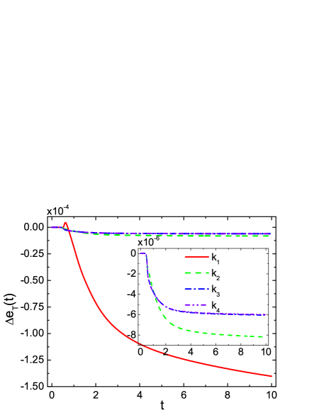
For comparisons, we verify the proposed FFT algorithm with the same problem described in Fig. 2 and display variations of total energy $\Delta e_{T}(t)$ obtained from WFFT schemes with $k_{1}$, $k_{2}$, $k_{3}$, and $k_{4}$ in Fig. 8. It is found that, for each case, $\Delta e_{T}(t)$ oscillates at the beginning, then approaches a nearly constant value. Behaviors of $\Delta e_{T}(t)$ can be interpreted as follows. At the beginning of phase separation, the fluids separate spontaneously into small regions with higher and lower densities, and more liquid-vapor interfaces appear. As a result, spacial discretization errors in Eq. (10) induced by interfaces arrive at their maxima that account for the initial oscillations. As time evolves, under the action of surface tension, the total liquid-vapor interface length decreases due to the mergence of small domains, then the discretization errors decrease. With the increase of precision, variations of total energy $\Delta e_{tol}(t)$ decreases. We can, therefore, come to the conclusion that WFFT scheme with higher-order filter has more advantage in guaranteeing energy conservation than the one with lower-order filter and other FD schemes used above.

4 Simulation results and analysis

In this section, two kinds of typical benchmarks are performed to validate the physical properties of the thermal multiphase model and the newly proposed algorithm. The first one is related to a planar interface. The second one is related to a circular interface.

4.1 Coexistence curve, spurious velocities and interfacial width

To check if the thermal LB multiphase model can correctly reproduce the equilibrium thermodynamics of the system and the numerical accuracy of the new scheme, a series of simulations about the liquid-vapor interface at different temperatures were performed. Unless otherwise stated, the WFFT scheme with $k_{4}$ is used throughout our simulations.

Simulations were carried out over a $512\times 4$ domain with PBC in both directions. The initial conditions are set as

$$\left\{\begin{array}[]{cc}(\rho\text{, }u_{x}\text{, }u_{y}\text{, }T)|_{L}=(\rho_{v}\text{, }0.0\text{, }0.0\text{, }0.97)\text{,}&x\leq N_{x}/4\text{;}\\ (\rho\text{, }u_{x}\text{, }u_{y}\text{, }T)|_{M}=(\rho_{l}\text{, }0.0\text{, }0.0\text{, }0.97)\text{,}&N_{x}/4<x\leq 3N_{x}/4\text{;}\\ (\rho\text{, }u_{x}\text{, }u_{y}\text{, }T)|_{R}=(\rho_{v}\text{, }0.0\text{, }0.0\text{, }0.97)\text{,}&3N_{x}/4<x\text{,}\end{array}\right.$$ (58)

where $\rho_{v}=0.80$ and $\rho_{l}=1.20$ are the theoretical values at $T=0.99$. Parameters are set to be $\tau=10^{-2}$, $K=0$ and others are unchanged. The initial temperature is set to be $0.97$, but dropping by $0.02$, when the equilibrium state of the system is achieved. Simulations were then run until the temperature had reduced to $0.87$.

Figure 9: (Color online) Comparisons of liquid-vapor coexistence curves from LB simulations and Maxwell construction. Here the surface tension parameter $K$ is set to be $0$.

Figure 10: (Color online) Velocity profiles obtained using various schemes at $T=0.93$ with $K=0$.

Figure 11: (Color online) Density profiles obtained using different schemes at $T=0.93$ with $K=0$.

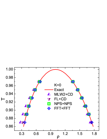
In Fig. 9, the liquid-vapor coexistence curves from LB simulations using various numerical schemes at different temperatures are compared to the theoretical predictions from Maxwell construction. One can see that when using the WFFT and the NPS schemes, the results are closer to the theoretical phase diagram. Nevertheless, when the temperature is lower than $0.87$, the NPS scheme becomes unstable. Physically, this is owing to the sharp interface when $K=0$ (see Fig. 11) and the nature of the VDW EOS, since large density ratio occurs when the temperature is much lower than the critical one. From another perspective, it demonstrates that the WFFT algorithm has a better numerical stability for this test. Results from the MLW2 and the FL schemes deviate remarkably from the theoretical values, especially for the vapor branch at lower temperatures. Besides physical reasons listed above, numerical accuracy of these two schemes is also an important factor.

Figure 12: (Color online) Velocity profiles obtained using various schemes at $T=0.93$ with $K=5\times 10^{-6}$.

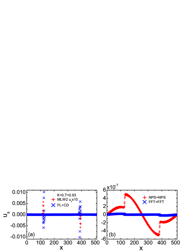
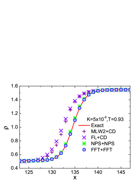
The velocity and density profiles at $T=0.93$ are shown in Fig. 10 and Fig. 11, respectively. As one can see in Fig. 10, for all schemes, spurious velocities exist and reach their maxima near the interface regions. However, the maximum spurious velocities obtained from different schemes are greatly different. For the MLW2 and the FL schemes, the maxima of $u^{s}$ are on the order of $10^{-4}$ and $10^{-2}$, respectively. A significant reduction of the $u^{s}$ is achieved by using the NPS scheme, decreasing the maximum to about $5\times 10^{-7}$. Through the usage of the WFFT algorithm, $u^{s}$ is further reduced by an order of magnitude compared to NPS scheme. Density profiles in Fig. 11(a) indicate that spurious interfaces (scatter symbols near the interfaces) have been produced when using the MLW2 scheme or the FL scheme because of excess numerical diffusion, which does not provide us a clear picture of phase separation, especially when the temperature is close to the critical value. This feature is not present when using the NPS scheme or the WFFT scheme (see Fig. 11b).

Figure 13: (Color online) Comparisons of coexistence curves from LB simulations and Maxwell construction. Here $K$ is set to be $5\times 10^{-6}$.

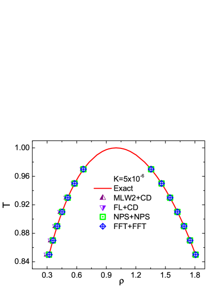
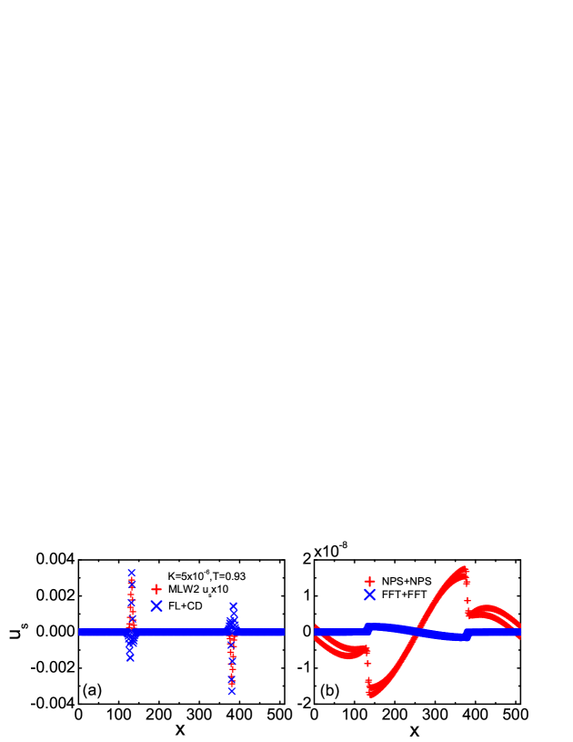
For all numerical schemes, the strength of surface tension plays an important role in reducing spurious velocities, as shown in Fig. 12. In the case of $K=5\times 10^{-6}$, the amplitudes of $u^{s}$ can be reduced by a factor of approximately $10$ with respect to the case of $K=0$. Subsequent simulations indicate that $u_{\max}^{s}$ will decrease to $10^{-12}$ when $K$ increases to $10^{-5}$. This is due to the existence of a wider interface and a smaller density gradient in the interface region when $K$ increases. With the decrease of spurious velocities, a more accurate phase diagram, especially in the vapor branch, is also achieved (see Fig. 13), even in the MLW2 case and the FL case.

Figure 14: (Color online) Velocity profiles obtained using various schemes at $T=0.85$ with $K=5\times 10^{-6}$.

Figure 15: (Color online) Equilibrium density profiles across liquid-vapor interface at $T=0.93$ with $K=5\times 10^{-6}$.

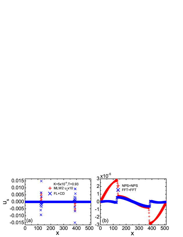
Besides the strength of surface tension, temperature is another key factor affecting spurious velocities, as displayed in Fig. 14. For all numerical schemes, a lower temperature makes larger spurious velocities. It is worth mentioning that, at the same temperature, the WFFT algorithm also allows to reduce $u^{s}$ of about an order of magnitude compared to NPS scheme.

In our simulations, so far, we have not discussed in detail the width of interface. According to the VDW theory, the interface width $l$, can be determined by numerically solving the following integral for a planar interface [61, 62]

$$l=x-x_{0}=-\frac{1}{\sqrt{2}(a/K)^{1/2}}\int_{\rho^{\ast}(x_{0}^{\ast})}^{\rho^{\ast}(x^{\ast})}\frac{d\rho^{\ast}}{[\Phi^{\ast}(\rho^{\ast})-\Phi^{\ast}(\rho_{l}^{\ast})]^{1/2}}\text{,}$$ (59)

where $\rho^{\ast}=\rho b$, $T^{\ast}=bT/a$ and,

$$\Phi^{\ast}=\rho^{\ast}\xi-\rho^{\ast}T^{\ast}[\ln(1/\rho^{\ast}-1)+1]-\rho^{\ast 2}\text{,}$$ (60)

$$\xi=T^{\ast}\ln(1/\rho_{s}^{\ast}-1)-\rho_{s}^{\ast}T^{\ast}/(1-\rho_{s}^{\ast})+2\rho_{s}^{\ast}\text{, }s=v\text{, }l$$ (61)

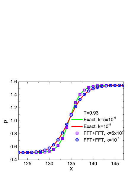
with $a=9/8$, $b=1/3$ in this model. Note that the solution of the above equations gives the exact density profile for a planar interface for any value of $T$. Equilibrium density profiles across the liquid-vapor interface at $T=0.93$ from LB simulations versus results from VDW theory are shown in Fig. 15. It is clear that although the liquid and the vapor densities calculated from the MLW2 and the FL schemes coincide with the theoretical ones, neither the MLW2 nor the FL scheme produces the correct interface profile. The wider interface in these two cases is due to the excess numerical diffusion, as shown in Fig.11a. The NPS approach leads to a small deviation from the VDW theory, while the WFFT scheme presents a perfect consistency with the theoretical solution. In Fig. 16 we display density profiles obtained from WFFT algorithm with $K_{1}=5\times 10^{-6}$ and $K_{2}=10^{-5}$, respectively. As expected, the interface becomes wider as $K$ increases. A wider interface decreases the density gradient in the interface region and helps to stabilize the liquid-vapor system at lower temperature.

Figure 16: (Color online) Equilibrium density profiles across the liquid-vapor interface at $T=0.93$ with $K_{1}=5\times 10^{-6}$ and $K_{2}=10^{-5}$.

4.2 Laplace’s law

Figure 17: (Color online) Evolution of a droplet from triangle to circle, where $t=0$ in (a), $t=0.1$ in (b), $t=1.5$ in (c), and $t=5.0$ in (d).

Figure 18: (Color online) Velocity fields at $t=30.0$ from the NPS scheme in (a) and the WFFT scheme with $k_{4}$ in (b).

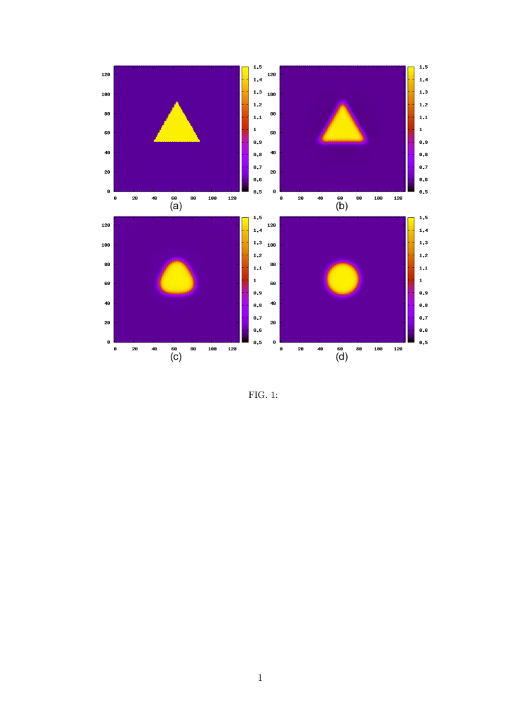
In this subsection, we will look at the dynamics of the relaxation of a deformed droplet driven by surface tension, and investigate the magnitude, as well as the spatial extent of the spurious currents for the circular interface. Initially, an equilateral triangular droplet with an initial sharp interface is placed at the center of the computational domain with $N_{x}=N_{y}=128$ lattice units. Initial conditions are given by

$$\left\{\begin{array}[]{l}(\rho\text{, }u_{x}\text{, }u_{y}\text{, }T)|_{in}=(1.46\text{, }0.0\text{, }0.0\text{, }0.95)\text{,}\\ (\rho\text{, }u_{x}\text{, }u_{y}\text{, }T)|_{out}=(0.58\text{, }0.0\text{, }0.0\text{, }0.95)\text{,}\end{array}\right.$$ (62)

where subscripts ‘in’ and ‘out’ indicate macroscopic variables inside and outside the liquid drop, respectively. PBC are employed on both the vertical and horizontal boundaries. The surface tension parameter is $K=10^{-5}$, leaving the others unchanged. After $3\times 10^{6}$ time steps, the system reaches equilibrium. Contour plots of the fluid density at four representative times are shown in Fig. 17. It is clearly seen that due to the effects of surface tension, the droplet relaxes to a circle slowly.

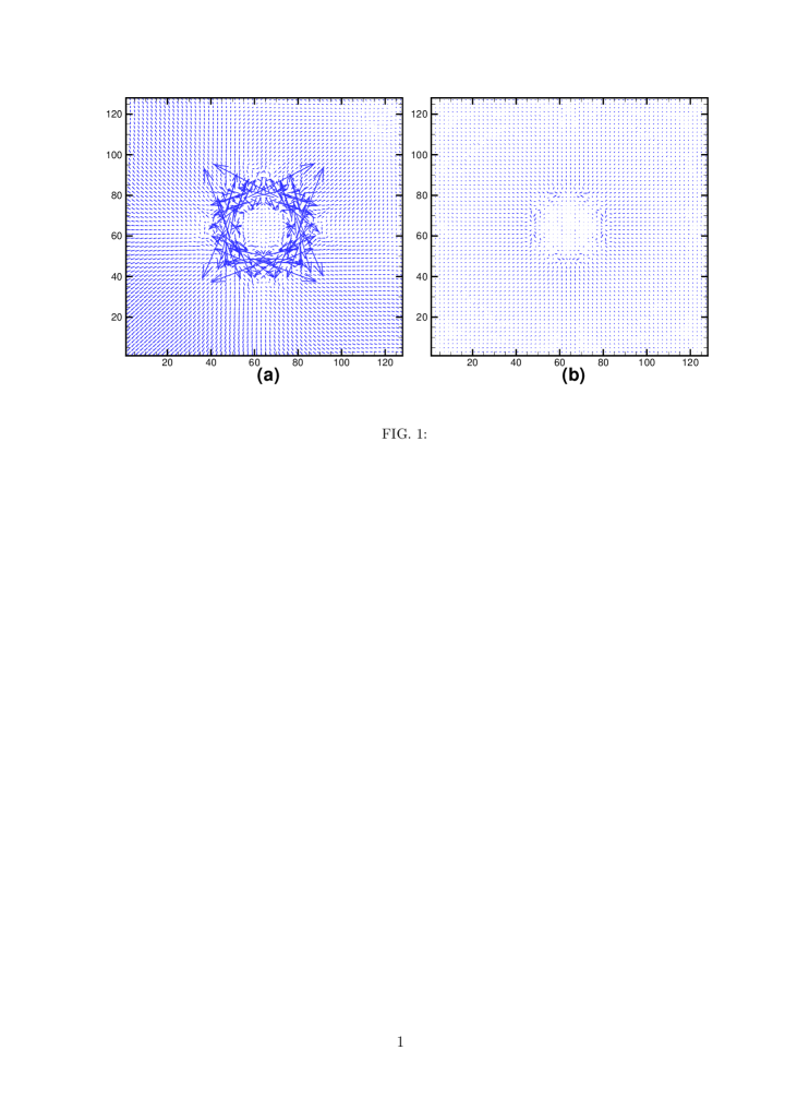
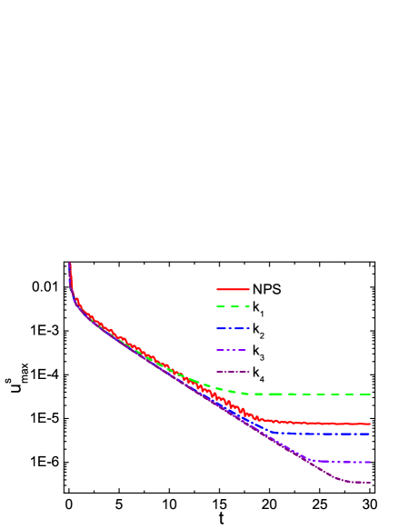
The velocity fields at $t=30.0$ obtained from the NPS scheme and the WFFT scheme with $k_{4}$ are plotted in Fig. 18. To illustrate the structure of the velocity field clearly, the lengths of the velocity vectors are multiplied by $5\times 10^{5}$. To be seen is that spurious currents exist in each case and are roughly aligned in the direction normally to the interface and rapidly disappear away from the interface. However, the magnitude of the spurious currents are significantly reduced as the WFFT approach is used. Figure 19 shows temporal evolution of the maximum velocity $u^{s}_{max}$ with the second-order, the fourth-order, the sixth-order, and the eighth-order FFT schemes, and the NPS scheme. We can see that, in each case, $u^{s}_{max}$ decreases, and tends to nearly a constant when $t>20$. More importantly, with the increase of precision, $u^{s}_{max}$ decreases. There is a decrease of a factor $22$ for the velocities when using the WFFT scheme with $k_{4}$ respect to the NPS scheme.

Figure 19: (Color online) Evolution of the maximum velocity $u^{s}_{max}$ versus time $t$ with the NPS scheme and the WFFT schemes with $k_{1}$, $k_{2}$, $k_{3}$, and $k_{4}$.

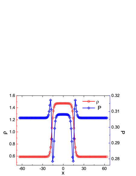
The density and the pressure profiles along the center line of the droplet are plotted in Fig. 20. In the inner and outer of the droplet, pressures $\bar{P}_{in}$ and $\bar{P}_{out}$ are two constants and a rapid change occurs across the interface. The difference between the two constants is usually used to compute the surface tension for a given $K$. For this purpose, we introduce the Laplace law which states

$$\sigma=r\Delta P=r(\bar{P}_{in}-\bar{P}_{out})\text{,}$$ (63)

where $\bar{P}_{in}$ is the mean pressure inside the droplet averaged over all points of $r_{in}<r/2$ from the droplet center and $\bar{P}_{out}$ is the external mean pressure averaged over all the points of $r_{out}>3r/2$. In this way, only the particles far from the interfaces are considered. Surface tension can also be computed in such a way [63, 64, 65]

$$\sigma=K\int_{-\infty}^{\infty}(\frac{\partial\rho}{\partial z})^{2}dz\text{.}$$ (64)

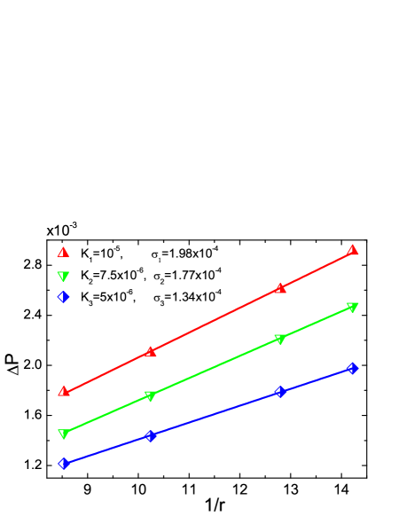
In order to test these relations, a series of simulations with sides ranging from $48$ to $81$ are run with three different surface tension parameters $K_{1}=10^{-5}$, $K_{2}=7.5\times 10^{-6}$ and $K_{3}=5\times 10^{-6}$.

Figure 20: (Color online) Density and pressure profiles along the center line of a droplet.

In Fig. 21, we present a plot of $\Delta P$ versus $1/r$ at $T=0.95$ and linear relation is well satisfied. By measuring the slope, the surface tension is found to be $\sigma_{1}=1.98\times 10^{-4}$, $\sigma_{2}=1.77\times 10^{-4}$, and $\sigma_{3}=1.34\times 10^{-4}$, which are in excellent agreement with the theoretical values, obtained from Eq. (55), $\sigma_{1}=1.96\times 10^{-4}$, $\sigma_{2}=1.72\times 10^{-4}$, and $\sigma_{3}=1.40\times 10^{-4}$. We mention that the relative error of surface tension $\varepsilon=\left|{\sigma_{LB}-\sigma_{exact}}\right|/\sigma_{exact}$ increases with the decrease of surface tension parameter. There are two reasons accounting for this behavior. Firstly, a larger $K$ will cause a larger surface tension and a larger pressure difference. This helps to measure the pressure difference with high accuracy. Secondly, when $K$ decreases larger spurious velocities will be produced and larger pressure oscillations will be induced.

Figure 21: (Color online) Laplace law tests for three different surface tension parameters. The scattered symbols are for simulation results and the dashed lines are linear fits of the scattered symbols.

5 Conclusions and discussions

In this paper, a thermal LB model for liquid-vapor system is developed. The present model experienced mainly three stages. It was originally composed by WT for ideal gas, then developed by GLS by adding an interparticle force term. Here we propose to use the WFFT scheme to calculate both the convection term and the external force term. The usage of the WFFT scheme is detailed and analyzed. It is found that the lower-order filters, with better numerical stability and lower accuracy, can effectively reduce the Gibbs phenomenon at discontinuity, while the higher-order filters help the scheme to maintain high resolution in smooth regions. One can choose appropriate filter according to the specific problem. With the higher-order WFFT algorithm, one can better control the non-conservation problem of total energy due to spatiotemporal disterizations. The model has been successfully applied to the calculation of interfacial properties of liquid-vapor systems. Very sharp interfaces can be achieved. By adopting the new model the magnitude of spurious currents can be greatly reduced. As a result, the phase diagram of the liquid-vapor system obtained from simulations are more consistent with that from theoretical calculation. The accuracy of the simulation results is also verified by the Laplace law.

Besides the numerical effects, both the surface tension and temperature have also significant influences on the spurious velocities. A stronger surface tension and/or a higher temperature can decrease the density gradient near the interfaces and stabilize the simulations. The analysis presented in this work provides an convenient way of extending the WFFT approach to multiphase LB models and to numerical solving partial differential equations. In further studies we will increase the depth of separation, which the model can undergo and investigate the similarities and differences between thermal and isothermal phase separations.

Appendix A Appendix: numerical accuracies of operators $k_{1}$, $k_{2}$, $k_{3}$, and $k_{4}$

Substituting Eq. (51) into Eq. (50), the RHS of Eq. (50) can be expressed as

$$\mathbf{i}k\times\widetilde{f}(k) = \frac{\mathbf{i}}{\Delta x/2}[\sin(k\Delta x/2)\times\widetilde{f}(k)$$ (65)

$$+\frac{1}{6}\sin^{3}(k\Delta x/2)\times\widetilde{f}(k)$$

$$+\frac{3}{40}\sin^{5}(k\Delta x/2)\times\widetilde{f}(k)$$

$$+\frac{5}{112}\sin^{7}(k\Delta x/2)\times\widetilde{f}(k)\cdots],$$

Taking IFT of the RHS of the first line of Eq. (65) gives

$$\texttt{IFT}[\mathbf{i}k_{1}\times\widetilde{f}(k)] = \frac{1}{L}\sum_{n=-N/2}^{N/2-1}e^{\mathbf{i}kx_{j}}\times\frac{\mathbf{i}}{\Delta x/2}\sin(k\Delta x/2)\times\widetilde{f}(k)$$ (66)

$$= \frac{1}{L}\sum_{n=-N/2}^{N/2-1}e^{\mathbf{i}kx_{j}}\frac{e^{\mathbf{i}k\Delta x/2}-e^{-\mathbf{i}k\Delta x/2}}{\Delta x}\times\widetilde{f}(k)$$

$$= \frac{f(x_{j}+\Delta x/2)-f(x_{j}-\Delta x/2)}{\Delta x}$$

$$= f^{\prime}(x_{j})+\frac{1}{24}\Delta x^{2}f^{\prime\prime\prime}(x_{j})+...$$

It is clear that the FFT scheme with operator $k_{1}$ has a second-order accuracy in space.

In a similar way, we have

$$\texttt{IFT}[\mathbf{i}k_{2}\times\widetilde{f}(k)]=f^{\prime}(x_{j})+\frac{1}{1920}\Delta x^{4}f^{(5)}(x_{j})+...,$$ (67)

$$\texttt{IFT}[\mathbf{i}k_{3}\times\widetilde{f}(k)]=f^{\prime}(x_{j})+\frac{1}{322560}\Delta x^{6}f^{(7)}(x_{j})+...,$$ (68)

$$\texttt{IFT}[\mathbf{i}k_{4}\times\widetilde{f}(k)]=f^{\prime}(x_{j})+\frac{1}{92897280}\Delta x^{8}f^{(9)}(x_{j})+...,$$ (69)

where $f^{(5)}(x_{j})$, $f^{(7)}(x_{j})$, and $f^{(9)}(x_{j})$ represent the fifth order, the seventh order, and the ninth order derivatives, respectively. Therefore, the WFFT approach with $k_{1}$, $k_{2}$, $k_{3}$, and $k_{4}$ has a second-order, fourth-order, sixth-order, and eighth-order accuracy in space, respectively.

From another perspective, it should be noted that, the FFT scheme is not a local scheme or, in other words, $k$ is not a local operator [55, 54], since each FFT coefficient is determined by all the grid point values of $f(x_{j})$, as shown in Eqs.(48-49). Therefore, the FFT scheme is not a finite-point formula, like the second-order FD is a 3-point formula, or the fourth order expression, is a 5-point formula; rather, the FFT scheme is $N$-point formulas. But there are important reasons for expressing derivatives as local operators. In a continuous space, the derivative of a function is defined locally. Hence, when modeling a continuous system with a discrete system, it is desirable to retain the local character of the derivative. This can be especially true near boundaries or marked internal inhomogeneities [54]. From the above derivations, we find that the FFT scheme with $k_{1}$ corresponds a 3-point FD scheme. Therefore, from the point of numerical analysis, $k_{1}$, $k_{2}$, $k_{3}$, and $k_{4}$ can maintain the local characteristic of $k$ in some extent. Hence, errors arising from the discontinuity are also localized and the accuracy away from the discontinuity can be ensured.

References

- [1] S. Succi, The Lattice Boltzmann Equation for Fluid Dynamics and Beyond, Oxford University Press, New York, 2001.
- [2] S. Chen, H. Chen, D. Martnez, W. Matthaeus, Phys. Rev. Lett. 67 (1991) 3776.
- [3] S. Succi, M. Vergassola, R. Benzi, Phys. Rev. A 43 (1991) 4521.
- [4] G. Vahala, B. Keating, M. Soe, J. Yepezand, L. Vahala, Comm. Comp. Phys. 4 (2008) 624.
- [5] A. Ladd, J. Fluid Mech. 271 (1994) 311.
- [6] O. Filippova, D. Hanel, Comput. Fluids 26 (1997) 697.
- [7] S. Succi, E. Foti, F. Higuera, Europhys. Lett. 10 (1989) 433.
- [8] Q. Kang, D. Zhang, S. Chen, Phys. Rev. E 66 (2002) 056307.
- [9] M. Watari, M. Tsutahara, Phys. Rev. E 67 (2003) 036306.
- [10] A. Xu, Europhys. Lett. 69 (2005) 214; A. G. Xu, Phys. Rev. E 71 (2005) 066706.
- [11] K. Qu, C. Shu, Y. Chew, Phys. Rev. E 75 (2007) 036706.
- [12] Q. Li, Y. He, Y. Wang, G. Tang, Phys. Lett. A 373 (2009) 2101.
- [13] Y. Gan, A. Xu, G. Zhang, X. Yu, Y. Li, Physica A 387 (2008) 1721.
- [14] F. Chen, A. Xu, G. Zhang, Y. Li, S. Succi, Europhys. Lett. 90 (2010) 54003; F. Chen, A. Xu, G. Zhang, Y. Li, Phys. Lett. A 375 (2011) 2129.
- [15] G. Yan, J. Comput. Phys. 161 (2000) 61.
- [16] J. Zhang, G. Yan, X. Shi, Phys. Rev. E 80 (2009) 026706.
- [17] A. Gunstensen, D. Rothman, S. Zaleski, G. Zanetti, Phys Rev A 43 (1991) 4320.
- [18] X. Shan, H. Chen, Phys. Rev. E 47 (1993) 1815; X. Shan, H. Chen, Phys. Rev. E 49 (1994) 2941.
- [19] M. Swift, W. Osborn, J. Yeomans, Phys. Rev. Lett. 75 (1995) 830; G. Gonnella, E. Orlandini, J. Yeomans, Phys. Rev. Lett. 78 (1997) 1695; A. Wagner, J. Yeomans, Phys. Rev. Lett. 80 (1998) 1429; D. Marenduzzo, E. Orlandini, J. Yeomans, Phys. Rev. Lett. 92 (2004) 188301; R. Verberg, C. Pooley, J. Yeomans, A. Balazs, Phys. Rev. Lett. 93 (2004) 184501; D. Marenduzzo, E. Orlandini, J. Yeomans, Phys. Rev. Lett. 98 (2007) 118102.
- [20] X. He, S. Chen, R. Zhang, J. Comput. Phys.152 (1999) 642; X. He, R. Zhang, S. Chen, G. Doolen, Phys. Fluids 11 (1999) 1143.
- [21] A. G. Xu, G. Gonnella, A. Lamura, Phys. Rev. E 67 (2003) 056105; A. G. Xu, G. Gonnella, A. Lamura, Phys. Rev. E 74 (2006) 011505; A. G. Xu, G. Gonnella, A. Lamura, G. Amati, F. Massaioli, Europhys. Lett. 71 (2005) 651.
- [22] M. Sbragaglia, R. Benzi, L. Biferale, S. Succi, K. Sugiyama, F. Toschi, Phys. Rev. E 75 (2007) 026702.
- [23] V. Sofonea, A. Lamura, G. Gonnella, A. Cristea, Phys. Rev. E 70 (2004) 046702; A. Cristea, G. Gonnella, A. Lamura, V. Sofonea, Commun. Comput. Phys. 7 (2010) 350.
- [24] D. Rothman, J. Keller, J. Star. Phys. 52 (1988) 1119.
- [25] H. Xi, C. Duncan, Phys. Rev. E 59 (1999) 3022.
- [26] A. Kalarakis, V. Burganos, A. Payatakes, Phys. Rev. E 65 (2002) 056702.
- [27] K. Premnath, J. Abraham, Phys. Rev. E 71 (2005) 056706; K. Premnath, J. Abraham, Phys. Fluids 17 (2005) 122105.
- [28] J. Hyväuoma, P. Raiskinmäi, A. Jäberg, A. Koponen, M. Kataja, J. Timonen, Phys. Rev. E 73 (2006) 036705.
- [29] J. Hyväuoma, T. Turpeinen, P. Raiskinm äi, A. Jäberg, A. Koponen, M. Kataja, J. Timonen, Phys. Rev. E 75 (2007) 036301.
- [30] A. Briant, A. Wagner, J. Yeomans, Phys. Rev. E 69 (2004) 031602.
- [31] H. Huang, D. Thorne, M. Schaap, M. Sukop, Phys. Rev. E 76 (2007) 066701.
- [32] K. Furtado, J. Yeomans, Phys. Rev. E 73 (2006) 066124.
- [33] V. Sofonea, K. Mecke, Eur. Phys. J. B 8 (1999) 99.
- [34] X. Nie, Y. Qian, G. Doolen, S. Chen, Phys. Rev. E 58 (1998) 6861.
- [35] R. Zhang, X. He, G. Doolen, S. Chen, Adv. Water Resour. 24 (2001) 461.
- [36] P. Yuan, L. Schaefer, Phys. Fluids 18 (2006) 042101.
- [37] A. Wagner, Int. J. Mod. Phys. B 17 (2003) 193.
- [38] A. Cristea, V. Sofonea, Int. J. Mod. Phys. C 14 (2003) 1251; A. Cristea, Int. J. Mod. Phys. C 17 (2006) 1191.
- [39] X. Shan, Phys. Rev. E 73 (2006) 044701; X. Shan, Phys. Rev. E 77 (2008) 066702.
- [40] T. Lee, P. Fischer, Phys. Rev. E 74 (2006) 046709.
- [41] T. Seta, K, Okui, J. Fluid Sci. Technol. 2 (2007) 139.
- [42] C. Pooley, K. Furtado, Phys. Rev. E 77 (2008) 046702.
- [43] C. Pooley, H. Kusumaatmaja, J. Yeomans, Phys. Rev. E 78 (2008) 056709.
- [44] G. Gonnella, A. Lamura A, V. Sofonea, Phys. Rev. E 76 (2007) 036703.
- [45] C. Brennen, Fundamentals of Multiphase Flow, Cambridge University Press, Cambridge, 2005.
- [46] A. Onuki, Physica A 314 (2002) 419.
- [47] A. Onuki, Phase Transition Dynamics, Cambridge University Press, Cambridge, 2002.
- [48] A. Onuki, Phys. Rev. Lett. 94 (2005) 054501; A. Onuki, Phys. Rev. E 75 (2007) 036304; R. Teshigawara, A. Onuki, Europhys. Lett. 84 (2008) 36003; R. Teshigawara, A. Onuki, Phys. Rev. E 82 (2010) 021603.
- [49] R. Liu, C. Shu, Some New Methods in Computational Fluid Dynamics, Science Press, Beijing, 2003 (in Chinese).
- [50] T. Lee, C. Lin, J. Comput. Phys 206 (2005) 16.
- [51] A. Tiribocchi, N. Stella, G. Gonnella, A. Lamura, Phys. Rev. E 80 (2009) 026701.
- [52] K. Liang, Methods of Mathematical Physics, Higher Education Press, Beijing, 1998 (in Chinese).
- [53] C. Canuto, M. Hussaini, A. Quarteroni, T. Zang, Spectral Methods in Fluid Dynamics, Springer-Verlag, London, 1987.
- [54] C. Birdsall, A. Langdon, Plasma Physics via Computer Simulation, Adam Hilger, Bristol, 1991.
- [55] J. Boyd, Chebyshev and Fourier Spectral Methods, DOVER Publications, New York, 2000.
- [56] S. Orszag, Phys. Rev. Lett 26 (1971) 1100.
- [57] G. Sod, J. Comput. Phys. 27 (1978) 1.
- [58] M. Hussaini, D. Kopriva, M. Salas, T. Zang, AIAA J. 23 (1985) 64.
- [59] Y. Sun, Y. Zhou, S. Li, G. Wei, J. Comput. Phys. 214 (2006) 466.
- [60] C. Shu, ICASE Report No. 97-65, NASA/CR-97-206253.
- [61] V. Bongiorno, H. Davis, Phys. Rev. A 12 (1975) 2213.
- [62] B. McCoy, H. Davis, Phys. Rev. A 20 (1979) 1201.
- [63] J. Rowlinson, B. Widom, Molecular Theory of Capillarity, Clarendon Press, Oxford, 1989.
- [64] T. Inamuro, N. Konishi, F. Ogino, Comput. Phys. Commun 129 (2000) 32.
- [65] T. Inamuro, T. Ogata, S. Tajima, N. Konishi, J. Comput. Phys. 198 (2004) 628.