Hierarchy of boundary driven phase transitions in multi-species particle systems

Abstract

Interacting systems with $K$ driven particle species on a open chain or chains which are coupled at the ends to boundary reservoirs with fixed particle densities are considered. We classify discontinuous and continuous phase transitions which are driven by adiabatic change of boundary conditions. We build minimal paths along which any given boundary driven phase transition (BDPT) is observed and reveal kinetic mechanisms governing these transitions. Combining minimal paths, we can drive the system from a stationary state with all positive characteristic speeds to a state with all negative characteristic speeds, by means of adiabatic changes of the boundary conditions. We show that along such composite paths one generically encounters $Z$ discontinuous and $2(K-Z)$ continuous BDPTs with $Z$ taking values $0\leq Z\leq K$ depending on the path. As model examples we consider solvable exclusion processes with product measure states and $K=1,2,3$ particle species and a non-solvable two-way traffic model. Our findings are confirmed by numerical integration of hydrodynamic limit equations and by Monte Carlo simulations. Results extend straightforwardly to a wide class of driven diffusive systems with several conserved particle species.

I Introduction

Systems of interacting particles out of equilibrium with more than one particle species find wide range of applications in biological, social and physical context Gunter (03), KoloFischer (2007), Frey09 (3). Remarkable phenomena occurring in these systems are the so-called boundary-driven phase transitions (BDPTs), e.g. phase transitions induced uniquely by changes of the boundary conditions Krug (1991). These transitions can be both of first and second order, depending on whether the order parameter (e.g. the stationary bulk density) changing discontinuously or continuously across the transition line. It has been demonstrated that in systems with one particle species the first order (discontinuous) BDPTs are governed by shocks dynamics, while the second order (continuous) BDPTs are governed by rarefaction waves Kolomeisky et al. (1998). In case of several particle species corresponding in the hydrodynamic limit to the hyperbolic systems of conservation laws, it was noted that the number of qualitatively different first-order BDPTs increases with the number of particle species Popkov (2007), a fact which is related to a complex structure of shocks in systems of conservation laws Lax (1973, 2006),Bressan (2000). However, generic properties of boundary driven phase transitions in multi-species driven particle systems are largely unknown. Also, the mechanisms governing stationary state selection are known for one-species systems Kolomeisky et al. (1998); Popkov and Schütz (1999), while for systems with several particle species such a knowledge is lacking.

The aim of the present paper is to show the existence of hierarchies of qualitatively different phase transitions in driven systems with several particle species, with open boundaries, and to provide a first classification of them. In particular we show that in systems with $K$ species of particles there are generically at least $K$ first order (discontinuous) and $K$ second order (continuous) qualitatively different phase transitions. We demonstrate that these phase transitions can be observed by driving the system from a stationary state with all positive characteristic velocities to a state with all negative characteristic velocities, by means of adiabatic changes of the densities at the boundaries. The kinetic mechanisms underlying the occurrence of first order BDPTs is ascribed to shock waves interactions (both among themselves and with boundaries) while the origin of second order phase transitions is shown to be connected with rarefaction waves. This leads to several physical implications which are confirmed by numerical simulations. In particular, we show that the existence of shock waves and the continuity of the flux across a first order BDPT allows us to predict the location of the stationary densities after their discontinuous change. Similarly, conditions of stability of rarefaction waves allows us to predict the location of the second order phase transition points along a specific path in parameter space. Also, it follows that the occurence of qualitatively different BDPTs is connected to the existence of different classes of shock waves and rarefaction waves in systems with several particle species. Continuous paths in parameter space along which sequences of $Z$ first order and $2(K-Z)$ second order transitions with ($Z$ $=0,1,...,K$) occur, are identified. We show that for each value of $Z$, there are $\binom{K}{Z}$ qualitatively different paths, each of them leading to a different set of transitions.

Our general approach is tested on ideal solvable models (e.g. which admit product steady states) as well as on more realistic (not exactly solvable) ones. For the former we derive hydrodynamic equations of motion and use the theory of shock and rarefaction waves for system of conservation laws for their investigation. For non-solvable models we recourse to Monte-Carlo simulations as principal tool of investigation. To simplify the presentation we concentrate in more detail on the case of two particle species but the results are discussed in a manner that the extension to the case of an arbitrary number of particle species becomes straightforward.

The plan of the paper is the following. In Section II we introduce multi-species particle models and their basic properties. In Sec. III we discuss hierarchies of BDPTs in multi-species systems and in Sec. IV we characterize the ”minimal path” along which any chosen (discontinuous or continuous) BDPT can be observed, taking as working examples the cases of one and two particle species ($K=1,2$). In Sec.s V and VI we discuss the basic mechanisms governing first and second order BDPTs in multi-species systems, respectively. In Sec. VIII we illustrate our approach for the case of a more realistic (not exactly solvable) model for bidirectional traffic, while in Sec. VII we discuss special paths for models with $K$ particle species along which sequences of BDPTs in the parameter space occur. Finally, Sec.IX serves for conclusions and for open problems.

II Multi-species particle models out of equilibrium

We consider a system, consisting of many interacting particles, dynamics of which is governed by a Master Equation, with the rates $\{\Gamma_{CC^{\prime}}\}$ of transition between the states $C$ and $C^{\prime}$, on a discrete lattice. We assume that there are $K\geq 1$ particle species conserved independently, and that one can construct a hydrodynamic limit, which has the form of a system of conservation laws, of the type

$${\frac{\partial\rho_{k}}{\partial t}}+{\frac{\partial j_{k}(\rho_{1},\rho_{2},...\rho_{K})}{\partial x}} =\varepsilon{\frac{\partial}{\partial x}}\left(\sum\limits_{k=1}^{K}B_{kj}\frac{\partial\rho_{j}}{\partial x}\right)$$ (1)

$${k} {=1,2,...,K.}$$

Here $\rho_{k}\left(x,t\right)$ denotes the averaged local density of the specie $k$, $j_{k}$ is the respective flux, $B_{ij}(\rho_{1},\rho_{2},...,\rho_{K})$ is the diffusion matrix, $\varepsilon$ is an infinitesimally small positive constant. The system is defined on a segment $x\in[0,1]$. At the ends of the segment, Dirichlet boundary conditions are imposed:

$$\rho_{k}[0]=\rho_{k,L},\text{ \ }\rho_{k}[1]=\rho_{k,R}.$$ (2)

We are interested in the stationary state of the system, i.e. in a state attained in the infinite time limit $t\rightarrow\infty$.  Note that in the case of perfect match between left and right boundary densities Eqs. (1),(2) allow stationary space-homogeneous solution $\rho_{k}(x)\equiv\rho_{k,L}=\rho_{k,R}$ for all $k$. Stability of this solution for all physical values of $\rho_{1},\rho_{2},...,\rho_{K}$ is guaranteed by the positive definiteness of the diffusion matrix $B_{ij}$. For the source particle model, this corresponds to an existence of a homogeneous stationary state with constant average particle densities $\rho_{1},\rho_{2},...,\rho_{K}$.

Some remarks are in order. Dirichlet boundary conditions (2) in terms of particle system mean that the system is coupled to boundary reservoirs with fixed particles densities $\rho_{k,L},\rho_{k,R}$ at the left and right ends, respectively. How this can be implemented or read off from boundary rates was discussed in Popkov and Schütz (2004). The flux $j_{k}(\rho_{1},\rho_{2},...,\rho_{K})$ is a nonlinear function of the particle densities, which implies interaction between particles. For a precise definition of the genuine flux nonlinearity see e.g. Lax (1973).

A special role is played by the Jacobian matrix of the flux ${\left(\mathcal{D}\mathbf{j}\right)}_{kw}=\partial j_{k}/\partial\rho_{w}$ whose eigenvalues $c_{1}<c_{2}<...<c_{K}$, called characteristic speeds, are all real and distinct Wea (note that we numerate the characteristic speeds in the increasing order). The characteristic speeds for the original particle system are velocities with which the local perturbations of a homogeneous state are propagating Popkov and Schütz (2003). The physical region (i.e. the region with physically meaningful particle densities $\rho_{k}$) splits into domains according to the signs of characteristic velocities. E.g. for $K=2$ we shall call $G_{-+}$ the domain in $u,v$ space ($u,v$ are particle densities of the two species) where $c_{1}(u,v)<0$ and $c_{2}(u,v)>0$. Characteristic speeds are smoothly-changing functions of particle densities. Special role is played by the subdomains of dimension $K-1$ across which, one of characteristic speeds changes its sign. E.g. the domains $G_{++}$and $G_{-+}$ are separated by the subdomain $G_{0+}$ with $c_{1}(u,v)=0$. An example of a decomposition of the physical region for $K=2$ is given in Fig.4. If a stationary state of a particle model has bulk particle densities $u_{stat},v_{stat}$ belonging to the $G_{++}$ region, we call it $G_{++}$ stationary state, etc.. Analogously, if the left boundary densities $u_{L},v_{L}$ belong to, say, $G_{-+}$ domain, we say that left boundary is of $G_{-+}$ type etc. The generalization to arbitrary number of particle species $K>2$ is obvious.

III Hierarchies of continuous and discontinuous BDPT

Different types of BDPTs can occur in these models. A discontinuous (first order) phase transition of the $p-th$ type is a transition between a stationary state with $c_{1},...,c_{p-1}<0,$ $c_{p},...,c_{K}>0$ and a stationary state where $c_{p}$ has changed its sign. E.g., for $K=2$, type $1$ and type $2$ discontinuous transitions are transitions between $G_{++}\leftrightarrows G_{-+}$ and $G_{-+}\leftrightarrows G_{--}$, respectively. Note that there is no direct transition between the $G_{++}$ and $G_{--}$ state. This is due to the strict hyperbolicity: there is no region, where $G_{++}$ and $G_{--}$ touch each other (the contrary would mean the existence of a weak hyperbolic point Wea ). Obviously, in systems with $K$ species $p$ can generically take values $p=1,2,...K$, leading to $K$ different types of discontinuous phase transitions.

The continuous (second order) phase transition of type $p$ is a transition between a stationary state with zero $p-th$ characteristic velocity, $c_{p}=0$, and a stationary state where $c_{p}$ is strictly positive or negative. The signs of other characteristic velocities $c_{q},q\neq p$ do not change across this transition. E.g. for $K=2$, transitions $G_{++}\leftrightarrows G_{0+},G_{0+}\leftrightarrows G_{-+}$ are of type $p=1$, while the transitions $G_{-+}\leftrightarrows G_{-0},G_{-0}\leftrightarrows G_{--}$ are of type $p=2$. Note that continuous transition of type $G_{0+}\leftrightarrows G_{-0}$ does not happen since the respective subregions have no intersection due to strict hyperbolicity.

(a)

(b)

Figure 1: A schematic diagram, showing minimal Ph1 path (bold lines) and Ph2 paths (thin lines) in parameter space (Panel (a)) and in physical region (Panel (b)). The Ph2 path is continuous both in parameter space and in physical region. The Ph1 path is continuous in parameter space but is discontinuous in physical region. Panel (a): The axes represent sets of boundary densities at the left and at the right boundary. The part of the Ph2 trajectory marked by dashed line indicate the rarefaction-wave governed stationary state,(see Sec.VI). The bold dotted line in the left upper corner marks the part of the Ph1 path, inside which a first order transition occurs, see Sec.V. Panel (b): Schematic evolution of the stationary densities along a Ph1 path (bold broken line) and a Ph2 path (thin line). Along the Ph1 path at least one discontinuous $p$-type phase transition is observed. Along the Ph2 path, a pinning and depinning to a state with zero characteristic velocity (two continuous phase transitions of $p$-type) are observed. The pinning and depinning point correspond to the ends of the dashed-marked Ph2 segment on Panel (a).

In systems with weak hyperbolic point, where such an intersection exists, a continuous transition $G_{0+}\leftrightarrows G_{-0}$ may become possible (see direct Ph2 path in Fig.11 (b)). In case of $K$ species, $p$ can generically take values $p=1,2,..K$, leading to $K$ different types of continuous (second order) transitions.

IV Minimal paths to observe BDPT

Here we describe the simplest path in parameter space along which a single first or second order phase transition is surely observed, in a system with $K$ species of particles. For this we introduce a parameter space of dimension $2K$, coordinates of which are given by the left and right boundary densities $\{\rho_{L}|\rho_{R}\}\equiv\{\rho_{1,L},\rho_{2,L},...,\rho_{K,L}|\rho_{1,R},...,\rho_{K,R}\}$. Each point of the parameter space represents some boundary conditions (2). Let us also define a physical region of dimension $K$ coordinates of which are average bulk particle densities $\rho_{1},\rho_{2},...\rho_{K}$. Each stationary state with bulk particle densities $\rho_{stat}\equiv\{\rho_{1}^{stat},\rho_{2}^{stat},...,\rho_{K}^{stat}\}$ is represented by a point in the physical region. The bulk stationary density will be our order parameter.

A path in parameter space is represented by a continuous curve $\Gamma(s)$ given by the left and right boundary densities $\{\rho_{L}(s)|\rho_{R}(s)\}$ along the path, parametrized by the running coordinate $0\leq s\leq$ $1,$ with $s=0$ and $s=1$ corresponding to the initial and final points of the path, respectively. For each value of $s$, we wait until the system reaches a stationary state (which we assume to be homogeneous in the bulk) and record the stationary bulk particle densities $\rho_{stat}(s)\equiv\{\rho_{1}^{stat}(s),\rho_{2}^{stat}(s),...,\rho_{K}^{stat}(s)\}$. Thus, each path $\Gamma(s)$ in parameter space of dimension $2K$ is mapped on a path $\rho_{stat}(s)$ in physical region of dimension $K$. The mapping $\Gamma(s)\rightarrow\rho_{stat}(s)$ is not invertible, because many different boundary conditions can lead to states with equal bulk stationary densities.

Consider two neighboring domains $G_{X}$ and $G_{Y}$ in the physical region $\rho_{1},\rho_{2},...\rho_{K}$ characterized by the following signs of the characteristic speeds $c_{i}(\rho_{1},\rho_{2},...\rho_{K})$:

$$G_{X}:c_{1}<...<c_{p-1}<0;\text{ \ \ }c_{K}>c_{K-1}>...>c_{p}>0,$$

$$G_{Y}:c_{1}<...<c_{p}<0;\text{ \ \ }c_{K}>c_{K-1}>...>c_{p+1}>0,$$ (3)

Note that both $G_{X},G_{Y}$ have dimension $K$ and that domain $G_{X}$ has one positive characteristic speed more than $G_{Y}$. We denote with $G_{X0Y}$ a subdomain of dimension $K-1$ separating domains $G_{X}$ and $G_{Y}$, given by:

$$G_{X0Y}:c_{1}<...<c_{p-1}<0;\text{ \ \ \ }c_{p}=0;$$

$$\text{ \ \ \ \ \ \ }c_{K}>c_{K-1}>...>c_{p+1}>0.$$

Phase transitions occur along paths which connect neigbouring domains. In the following we denote by $\rho_{L}^{ini},\rho_{R}^{ini}$ the sets of the particle densities in the left and right boundary reservoirs at the initial point $s=0$ of a path $\Gamma(s)$, i.e. $\rho_{L}^{ini}\equiv\{\rho_{k,L}(s=0)\}_{k=1}^{K}$ ,  $\rho_{R}^{ini}\equiv\{\rho_{k,R}(s=0)\}_{k=1}^{K}$, $\Gamma(s=0)\equiv\{\rho_{L}^{ini}|\rho_{R}^{ini}\}$. Analogously, denote $\rho_{L}^{final},\rho_{R}^{final}$ the respective boundary densities at the end of the path $\Gamma(s=1)\equiv\{\rho_{L}^{final}|\rho_{R}^{final}\}$. Let us choose the initial  and the final boundary densities on both boundaries from domains $G_{X}$    and $G_{Y}$, respectively,

$$\rho_{L}^{ini}\in G_{X},\rho_{R}^{ini}\in G_{X}\text{ \ and }\rho_{L}^{final}\in G_{Y},\rho_{R}^{final}\in G_{Y}.$$ (4)

In addition, we shall choose the initial and the final boundary densities fully matching, $\rho_{L}^{ini}\equiv\rho_{R}^{ini}=\rho_{INI}$, and $\rho_{L}^{final}\equiv\rho_{R}^{final}=\rho_{FIN}$. Since the full match allows for trivial homogeneous stationary solution of (1),(2), the initial and final stationary states along the path belong to different $G$ domains: $\rho_{stat}(s=0)=\rho_{INI}\in G_{X}$ and $\rho_{stat}(s=1)=\rho_{FIN}\in G_{Y}$, see discussion after Eq.(2). Note that the condition of the full match can be relaxed (for an example see Sec.VIII), and is chosen here for simplicity of presentation.

Having chosen the initial and final points of a path $\Gamma(s)$, let us now define paths $\Gamma^{Ph1}(s),$ $\Gamma^{Ph2}(s)$ of type Ph1 and Ph2 as consisting of two consecutive elementary steps:

$$\Gamma^{Ph1}(s) :\{\rho_{L}^{ini}|\rho_{R}^{ini}\}\rightarrow\{\rho_{L}^{ini}|\rho_{R}^{final}\}\rightarrow\{\rho_{L}^{final}|\rho_{R}^{final}\},$$ (5)

$$\Gamma^{Ph2}(s) :\{\rho_{L}^{ini}|\rho_{R}^{ini}\}\rightarrow\{\rho_{L}^{final}|\rho_{R}^{ini}\}\rightarrow\{\rho_{L}^{final}|\rho_{R}^{final}\}.$$ (6)

During each elementary step the boundary densities at one boundary change adiabatically while the other boundary is kept fixed. We shall call an elementary step during which the left (the right) boundary densities change a step L ( step R), respectively. Thus, a Ph1 path $\Gamma^{Ph1}(s)$ consists of consecutive steps step R $\rightarrow$ step L, while in a Ph2 path the steps R and L are interchanged, see Fig. 1. It is important that a domain $G_{X}$ of departure for both paths has more more positive characteristic velocities than the domain of arrival $G_{Y}$, the reason for which will be explained in the next section.

We assume trajectories $\rho_{R}^{ini}\longrightarrow\rho_{R}^{final}$ (step R) and $\ \rho_{L}^{ini}\longrightarrow\rho_{L}^{final}$ (step L) to lie entirely inside $G_{X}$ and $G_{Y}$, and to cross $c_{p}=0$ hyperplane only once, see Fig.1 (a). The main results of this section are presented in the two propositions listed below.

Proposition I. Discontinuous change of the stationary density $\rho_{stat}$ from a point in domain $G_{X}$ to a point in neighboring domain $G_{Y}$ ($p-$th type of first order transition) occurs along any Ph1 path (5) connecting these domains.

(a)

(b)

Figure 2: Panel (a): Phase diagram of TASEP with open boundaries. LD, HD and MC denote Low Density, High Density and Maximal Current phases respectively. Thick(thin) lines separating different phases mark phase transitions of the first ( of the second) order. Thick and thin lines originating in INI point (0.3,0.3) and ending in FIN points show Ph1 and Ph2 paths, respectively. Panel (b): Stationary densities along the Ph1 path(bold line) and along the Ph2 path (thin line) shown on Panel (a), versus running variable $s$, parametrizing the paths. A cusp in the upper part of the Ph1 density path $u_{stat}(s)$ results from a cusp in the Ph1 path in parameter space(Panel a).

The path $\Gamma^{Ph1}(s)$ is continuous in the parameter space coordinates of which are left and right boundary densities. We claim that at some point $s^{\ast}$ whose precise location depends on the microscopic transition rates, the stationary density $\rho_{stat}(s)$ undergoes discontinuous jump (a first order transition) from some value $X\in G_{X}$ (non necessarily coinciding with initial point $\rho^{ini}$) to a value $Y\in G_{Y}$ (non necessarily coinciding with end point $\rho^{final}$). The stationary flux across the transition is continuous, $j_{stat}(X)=j_{stat}(Y)$.

Proposition II: Two continuous (second order) phase transitions of type $p$ are observed along any path of type Ph2. Those transitions are continuous phase transitions $G_{X}\rightarrow G_{X0Y}$ and $G_{X0Y}\rightarrow G_{Y}$.

Figure 3: Multi-chain model and two-way traffic model on a narrow road. Coupling to boundary reservoirs is indicated by boxes marked L (left reservoir) and R (right reservoir).

Summarizing Propositions I and II, we have that by proceeding along Ph1 (Ph2) path connecting two stationary states in neighboring regions, we observe one first order (two second order) transitions between these states (see Fig.1). Alternatively, one can say that any Ph1 path in parameter space maps onto a discontinuous path $\rho_{stat}(s)$ in physical region, while any Ph2 path in parameter space maps onto a continuous path $\rho_{stat}(s)$ in the physical region, a segment of which is pinned to the $c_{p}=0$ hyperplane, see Fig.1. Continuous phase transitions $G_{X}\rightarrow G_{X0Y}$ and $G_{X0Y}\rightarrow G_{Y}$ correspond to pinning and depinning points of the Ph2 trajectory. We remark that in particle systems without hysteresis the above paths are fully invertible, i.e. by proceeding along a path $\Gamma(s)$ in the opposite direction from the final to initial point, one encounters exactly the same mapping $\Gamma(s)\rightarrow\rho_{stat}(s)$.

The physical significance of the Ph2 path resides in the fact that it contains favourable boundary setups for the formation of rarefaction waves governing the $G_{X0Y}$-type stationary states (Ph2 segment marked in Fig.1(a) by dashed line) and does not contain boundary setups favoring stable shock waves which govern discontinuous phase transitions. Consequently, discontinuous shock-wave driven transitions are impossible along any Ph2 path and the mapping $\Gamma(s)\overset{Ph2}{\rightarrow}\rho_{stat}(s)$ is continuous (see also sec.VI). Analogously, one can deduce that the mapping $\Gamma(s)\overset{Ph1}{\rightarrow}\rho_{stat}(s)$ along any Ph1 path must be discontinuous. More details are given in Secs.V,VI. Before discussing the kinetic mechanisms underlying the transitions we illustrate Propositions I and II with some specific examples.

Case K=1. It is instructive to start with the simplest possible and well known case of one particle species $K=1$. Let us take the Totally Asymmetric Simple Exclusion Process, or TASEP Schütz (2000),Derrida (1998) as a representative. This process is defined on a chain, each site of which can be empty or occupied by one particle. Particles jump independently after an exponentially distributed random time with mean $1$ to a nearest neighbor site on the right, provided that the target site is empty (hard core exclusion rule). We recall that the particle flux, which is a number of particles crossing a single bond per unit time, as function of the density $u$ for this model has the form $j(u)=u(1-u)$ and the physical region of densities is $0\leq u\leq 1$ due to the hard core exclusion.

Figure 4: Decomposition of the physical domain for a model with two species [ multi-chain model with $K=2,\gamma=0.5$, see text for model definition], according to signs of characteristic speeds $c_{1},c_{2}$. E.g. $G_{0+}$ denotes region where $c_{1}=0,\ c_{2}>0$ etc.. Points $A,B,C,D$ are reference points in respective $G$-domains, chosen for illustration of Ph1 and Ph2 paths in Figs.5,6.

The characteristic speed $c=j^{\prime}(u)=1-2u$ is positive for $u\in[0,1/2)$, is negative for $u\in(1/2,1]$, and it vanishes for $u=1/2$, thus defining the respective domains $G_{+},G_{-}$ and $G_{0}$. The boundary densities are $u_{L}$ and $u_{R}$. The well-known stationary states of TASEP with open boundaries, the Low Density (LD) state, the High Density (HD) state, and the Maximal Current (MC) state are readily identified with $G_{+}$, $G_{-}$ and $G_{0}$ states, respectively. The phase diagram of TASEP and the mappings $\Gamma(s)\rightarrow u_{stat}(s)$ for Ph1- and Ph2-paths are shown in Fig.2. Note that along the Ph1 path one encounters a discontinuous phase transition from LD to HD state $G_{+}\rightarrow G_{-}$. Along the Ph2 path two continuous phase transitions $G_{+}\rightarrow G_{0}$ , $G_{0}\rightarrow G_{-}$ take place.

Case K=2. As examples we choose a multi-chain model Popkov and Salerno (2004) restricted to $K=2$, and a two-way traffic model on a narrow road. The former describes interacting exclusion processes evolving on parallel chains with species hopping in the same direction, while the latter describes the exclusion process with species hopping in opposite direction, see Fig.3. Both models are described in continuous limit by equations of type (1),(2).

The multi-chain model is solvable on a ring, its stationary current is known analytically together with the diffusion matrix $B$, this giving the possibility of using either hydrodynamic limit equations (1) or microscopic approach (Monte Carlo simulations). Moreover, it is known from previous studies Popkov (2004), Popkov and Salerno (2004), that numerical integrations of the respective discretized hydrodynamic equations (1), (2), reproduce very accurately (if not exactly) the outcome of the respective Monte-Carlo simulations. The other model (two way traffic) is not solvable and Monte Carlo simulations remain the only tool of investigation.

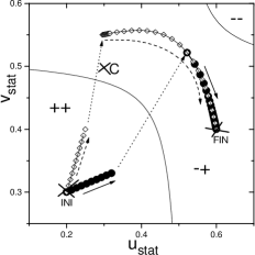
(a)

(b)

Figure 5: Location of stationary densities for two-chain model ($\gamma=0.5$) for (a) two alternative Ph1 paths (b) two alternative Ph2 paths from $G_{++}$ to $G_{-+}$ domains. Initial and end points for all paths corresponds to fully matching left-right boundary densities $\rho_{ini}=(0.2,0.3)$, $\rho_{final}=(0.6,0.4)$ (points A,B in Fig.4). Path I (filled symbols) is a direct path $\rho_{ini}\rightarrow\rho_{final}$, where the boundary densities during respective steps L and R (see Sec.IV) change by linear interpolation, e.g. $u_{R}(s)-u_{R}^{ini}=(u_{R}^{fin}-u_{R}^{ini})s$, etc.. Path II (open symbols) goes through intermediate point C with coordinates $\rho_{C}=(0.3,0.5)$ i.e. each step L,R involves sequence of two linear interpolations $\rho_{ini}\rightarrow\rho_{C},\rho_{C}\rightarrow\rho_{final}$. Evolution of the densities along the paths I and II is indicated by solid and dashed arrows, respectively, crosses mark initial, intermediate and final points. Data points are taken from numerical integration of the respective discretized hydrodynamic equations (1),(2). Deviations from the exact $c_{p}=0$ line in Panel (b) are due to finite-size errors.

First consider the multi-lane model for $K=2,$ see the top panel of Fig.3. The only allowed move is a hopping of a particle to its nearest neighbouring site on its right, with the rate $r_{n}=1-n\gamma/2$ where $0\leq n\leq 2$ is the number of particles on the adjacent chain, neigbouring to the departure and to the target site (see Fig.3). The interchain interaction parameter $\gamma$ varies from $\gamma=0$ (corresponding to two uncoupled TASEPs ) to $\gamma=1$ (maximal interaction). Particle hopping obeys the exclusion rule: if the target site is already occupied, the move is rejected. The hopping between chains is not allowed. We denote the average density of particles on the first and second chain as $u,v$, respectively. Due to hardcore exclusion, the physical region of densities for this model is the square domain $0\leq u,v\leq 1$. The model has product stationary states, which allows to calculate stationary currents Popkov and Salerno (2004) $j_{u}=u(1-u)(1-\gamma v)$ and $j_{v}=v(1-v)(1-\gamma u).$ The characteristic velocities $c_{k}$ are the eigenvalues of the flux Jacobian $(D\mathbf{j})\varphi_{k}=c_{k}\varphi_{k}$, where

$$D\mathbf{j}=\begin{pmatrix}(1-2u)(1-\gamma v)&-\gamma u(1-u)\\ -\gamma v(1-v)&(1-2v)(1-\gamma u)\end{pmatrix}.$$ (7)

Consistently with our notations, a domain in $u,v$ plane with $c_{1}(u,v)>0,$ $c_{2}(u,v)>0$ will be denoted by $G_{++}$ (and similarly for other sign combinations). For generic interaction $\gamma<1$, all domains $G_{++},G_{-+},G_{--}$ are present, see Fig.4. As $\gamma$ increases, the domain $G_{--}$ shrinks and for $\gamma=1$ (maximal interaction) it disappears completely.

According to the Proposition I, described in the Sec.IV, starting from the domain $G_{++}$ and going to the domain $G_{-+}$ using a Ph1 path (5), we should observe discontinuous transition in stationary density along the path. In Fig. 5(a) stationary densities along two alternative Ph1 paths between the same initial point (located in $G_{++}$) and final point (located in $G_{-+}$) are shown. These paths, indicated as $AB$ and $ACB$ in Fig.4, differ by the elementary trajectories $\rho_{ini}\rightarrow\rho_{final}$ are built, see caption of Fig.5(a). As expected, the qualitative scenario does not depend on the details of the path: in both cases we see a discontinuous transition $G_{++}\rightarrow G_{-+}$. Similarly, along the two alternative Ph2 paths (6) two continuous BDPT occur: $G_{++}\rightarrow G_{0+}$ and $G_{0+}\rightarrow G_{-+}$ (see Fig.5(b)), in accordance with the Proposition 2.

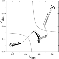
(a)

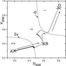
(b)

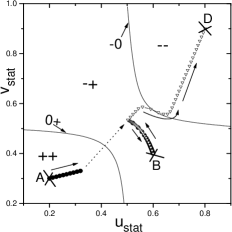
(c)

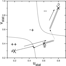
(d)

Figure 6: Panels (a)-(d): Location of stationary densities for two-chain model with $\gamma=0.5$ along (Ph1)(Ph1),(Ph2)(Ph2),(Ph1)(Ph2), and (Ph2)(Ph1) paths, respectively. All trajectories pass through initial (A), middle (B) and final (D) points. E.g. Panel (b) shows stationary densities along two consecutive Ph paths $A\rightarrow^{Ph1}B$,$B\rightarrow^{Ph2}D$. Filled (empty) symbols mark stationary densities $u_{stat},v_{stat}$ along the first (the second) Ph path. Evolution of the densities along the path is shown by arrows. Along every Ph2 piece a pinning to/depinning from $c_{p}=0$ line is observed (two continuous phase transitions). Along every Ph1 piece a discontinuous phase transition occurs, marked by dotted arrows.

IV.1 Building composite paths

From the point B in $G_{-+}$ where all above described minimal paths ended, we can continue further building Ph1 $G_{-+}\overset{Ph1}{\rightarrow}G_{--}$ (5) or Ph2 $G_{-+}\overset{Ph2}{\rightarrow}G_{--}$ (6) paths to some point D in $G_{--}$, see Fig.4.

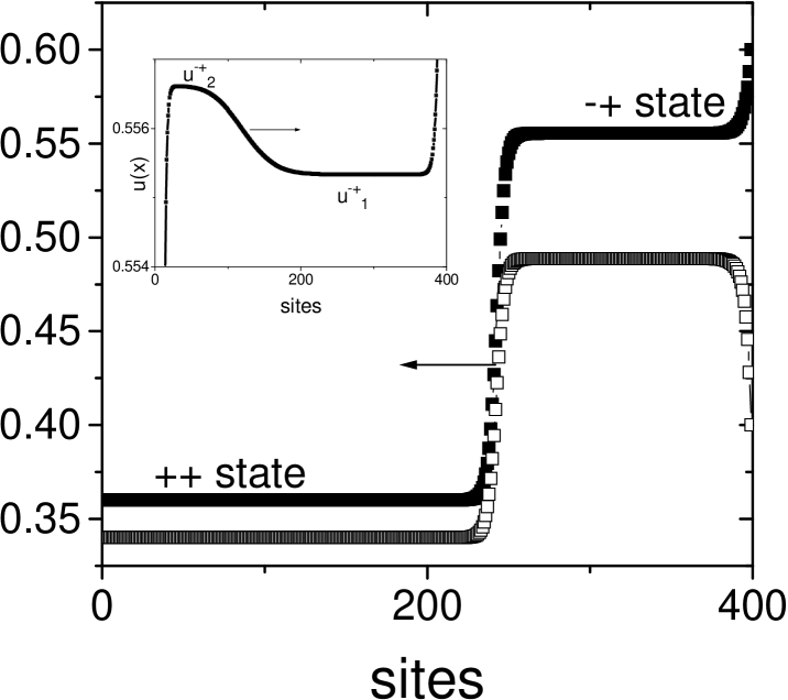
Figure 7: Average density profiles $u(x,t),v(x,t)$ evolution close to the first order phase transition line. Initial state at $t=0$ is a state matching the left boundary $u_{L}=0.36,v_{L}=0.34$(the right boundary is $u_{R}=0.6,v_{R}=0.4$). As time goes on, a shock wave at the right boundary appears and starts to propagate, its position at $t=6400$ is shown. After reaching the left boundary, it reflects, see Inset, taken at $t=17600$. Final stationary state has densities $u=0.5568,v=0.4868$.

Along the new Ph1 (Ph2) path from B to D we shall see another discontinuous (continuous) transition in the stationary density. Combining all possible Ph1 and Ph2 paths leading from $G_{++}$ $\rightarrow G_{-+}\rightarrow$ $G_{--}$, one can observe a desired sequence of phase transitions. E.g. choosing   only Ph1 paths $G_{++}\overset{Ph1}{\rightarrow}G_{-+}\overset{Ph1}{\rightarrow}G_{--}$, we see two phase transitions of the first order, see Fig.6(a). Along a path $G_{++}\overset{Ph2}{\rightarrow}G_{-+}\overset{Ph1}{\rightarrow}G_{--}$ we see two continuous transitions $G_{++}\rightarrow G_{0+}\rightarrow G_{-+}$ and a discontinuous transition $G_{-+}\rightarrow G_{--}$, etc.. The outcome of all four possible choices of composite paths passing from $G_{++}$ to $G_{--}$ are shown in Figs.6(a)-6(d).

IV.2 BDPTs for arbitrary number of species

The generalization of these considerations to systems with arbitrary number of species is straightforward. In systems with $K$ particle species, one can construct composite paths leading from a state with all positive characteristic speeds $G_{+...+}$ to a state with all negative characteristic speeds $G_{-...-}$, similarly to those shown in Figs.6(a)-6(d). Every composite path consists of $K$ consecutive minimal Ph1 or Ph2 paths, described in Sec.IV. Obviously, the number of qualitatively different composite paths is $2^{K}$. Along any composite path from $G_{+...+}$ state to $G_{-...-}$ state we shall observe at least $Z$ first order transitions, and at least $2(K-Z)$ discontinuous phase transitions, where $Z$ is the number of  Ph1 pieces in the composite path. We say ”at least”, because e.g. the number of first order transitions can occasionally be larger than $Z$ (in case of complicated shape of $G$-domains or if composite path crosses the same hyperplane $c_{p}=0$ several times), but not smaller than $Z$, and analogously for second order transitions.

Figure 8: Schematic picture of a shock waves interaction scenario for two-species system. Dashed line denote multiple reflections of the $-+$ shock from the boundaries, during which the bulk density exponentially converges to its stationary value.

E.g. already in one-component systems with a double maximum in the current-density relation $j(u)$, both $G_{+}$ and $G_{-}$ domains consist of two separated segments and a Ph1 path between disjoint $G_{+}$ and $G_{-}$ domains may lead to observation of two discontinuous transitions. In the next two sections we discuss the kinetic mechanisms governing BDPTs along minimal Ph1 and Ph2 paths.

V Shock wave mechanism underlying first order BDPT

Consider the first order phase transitions shown in Fig.5(a) from the $G_{++}$ to $G_{-+}$ state. Initial $G_{++}$ state is a state perfectly matching the left boundary. Note that the perfect match with the left boundary is the only possible way for a $G_{++}$ state to be stationary because any eventual perturbation at the left boundary will be carried away from it since both characteristic velocities are positive (see also Popkov (2007)). As we cross a transition point (at a small but finite distance from it) a new $-+$ shock wave with densities $u_{1}^{-+},v_{1}^{-+}$ belonging to $G_{-+}$ appears at the right boundary and starts to propagate inside the bulk. Note that the new shock does not match the right boundary $u_{1}^{-+}\neq u_{R},v_{1}^{-+}\neq v_{R}$) but forms a boundary layer with it (see Fig.7). The densities $u_{1}^{-+},v_{1}^{-+}$ are not the final stationary densities yet. After hitting the left boundary the shock reflects and changes its density to another value, $u_{2}^{-+},v_{2}^{-+}$ , see Fig. 7. This reflected wave, in its turn, hits the right boundary, reflects again and changes its density to $u_{3}^{-+},v_{3}^{-+}$.

This process continues indefinitely and the sequence $\{u_{n}^{-+},v_{n}^{-+}\}$ converges exponentially to the stationary value $u_{stat}^{-+},v_{stat}^{-+}$ as $n\rightarrow\infty$. The shock densities $u_{n}^{-+},v_{n}^{-+}$ for odd $n=1,3,...$ (for even $n=2,4,...$) belong to the right reflection map defined by $u_{R},v_{R}$ (to the left reflection map defined by $u_{L},v_{L}$), see Popkov (2004), Popkov and Schütz (2004) for more details. In practice, it becomes harder and harder to observe reflections of high order since the respective shocks differ by an infinitesimal change of densities (see inset of Fig.7). The sequence $\{u_{n}^{-+},v_{n}^{-+}\}$ , (unlike the fact of a presence of first order transition along the Ph1 path) is microscopic rates dependent, through the diffusion matrix $B$ from (1).

It is important to stress that precisely at the transition point the shock wave between the $++$ state (matching the left boundary $u_{L},v_{L}$) and the $-+$ state with densities $u_{1}^{-+},v_{1}^{-+}$ is unbiased, meaning that there is a perfect balance between the respective currents: $j_{u}(u_{L},v_{L})=j_{u}(u_{1}^{-+},v_{1}^{-+}),$ $j_{v}(u_{L},v_{L})=j_{v}(u_{1}^{-+},v_{1}^{-+})$. The fact that $c_{1}(u_{L},v_{L})>0$ ($c_{1}(u_{1}^{-+},v_{1}^{-+})<0$) at the left (right) from shock discontinuity guarantees the stability of the unbiased shock $G_{++}/G_{-+}$. At one side of the phase transition this shock is biased to the right leading to $G_{++}$ stationary state, and at another side of the phase transition it is biased to the left leading to $G_{-+}$ stationary state. This feature is essentially the same as in one-species systems, see Kolomeisky et al. (1998). Precisely at the phase transition line the unbiased shock performs a random walk between the boundaries. By averaging the local particle density over large times one samples configurations with the shock at all possible positions, which leads to a density profile with a linear slope, observed in Monte Carlo simulations (not shown for brevity).

More complicated scenarios at first order transition points may be observed if we choose left and right boundary densities belonging to non-connected $G$ domains (e.g. the left boundary belongs to $G_{++}$ and the right boundary belongs to $G_{--}$ domain), and impose flat initial conditions matching one of the boundaries, e.g. the left boundary of $G_{++}$ type. Close to the phase transition $G_{-+}$ $\rightarrow$ $G_{--}$ shown at Fig.10 along a single big Ph1 path, we shall see appearance of two shocks at the right boundary of $++/-+$ and of $-+/--$ type. For a while in the system there are two moving consecutive shocks.

Stability of such a  multi-shock is possible due to existence of two conserved quantities, see Lax (1973). The first shock reaches the left boundary and reflects from it (with changed densities). Now we have two shocks which counter-propagate and collide at some point, forming a single shock of $-+/--$ type. The future stationary state is then determined by the direction of motion of this shock: for positive (negative) shock velocity the resulting stationary state will be of $-+$ (of $--$ type). Again, we see that the first order phase transition is caused by the direction of the bias of a shock connecting two states. The schematic space-time evolution of the above described scenario is shown in Fig.8. Note, however, that if we follow an adiabatic path, the initial conditions as we have imposed will not appear (close to a transition point $G_{-+}$ $\rightarrow$ $G_{--}$ the initial state, to be quasi-stationary, must be either of $G_{-+}$ or of $G_{--}$ type), and consequently at any time we shall see at most one shock in the system.

This scenario of the first order phase transitions described above for two particle species is straightforwardly generalizable to an arbitrary number of species $K$. A discontinuous phase transition of the type $p$ (see Sect.III) along the minimal path described in Sec.IV is caused by a shock $G_{X}/G_{Y}$ between a $G_{X}$ state on the left from discontinuity and a $G_{Y}$ state on the right from discontinuity. State $G_{X}$ has one extra positive characteristic speed ($c_{p}>0$) with respect to the $G_{Y}$ state ($c_{p}<0$), see (3).

${}_{\begin{tabular}[c]{|l|l|l|l|l|l|}\hline\cr Left boundary&$++$ $\rightarrow$&$++$ $\rightarrow$&$++$ $\rightarrow$&$0+$ $\rightarrow$&$-+$\\ \hline\cr Right boundary&$++$ $\rightarrow$&$0+$ $\rightarrow$&$-+$ $\rightarrow$&$-+$ $\rightarrow$&$-+$\\ \hline\cr Stationary bulk&$++$&$++$&$++/-+$&$-+$&$-+$\\ \hline\cr\end{tabular}}$

Table 1: Sequential changes of the stationary state densities along a minimal path Ph1 (5) from $G_{++}$ to $G_{-+}$.

The signs of all remaining characteristic speeds (but not the characteristic speeds themselves) are the same at both sides of the shock. At the transition point, the shock $G_{X}/G_{Y}$ is unbiased (has zero velocity) and its stability is guaranteed by the fact that $c_{p}>0$ ($c_{p}<0$) on the left (on the right) from the discontinuity. Such a shock is called a $p$-shock in the PDE theory of conservation laws Lax (1973). Zero shock velocity signalizes equality of particle currents of all species at both sides of discontinuity. Consequently, the stationary current is continuous across the transition.

At one side of the transition, the $G_{X}/G_{Y}$ shock is biased to the right and then the $G_{X}$-type stationary state prevails. At the other side of the transition the shock is biased to the left, resulting in the $G_{Y}$-type stationary state. Thus, the density changes discontinuously at the transition point while the current is continuous (usually it has a cusp) across the transition point. The location of the transition point itself can be indicated on the respective Ph1 path only approximately, as being inside the dashed-like decorated segment of it, see Fig.1(a)) and Table 1.

If the left and right boundary densities belong to non-connected $G$ domains (but the number of positive characteristic speeds at the left boundary is larger than those at the right boundary) and if the initial state of the system matches one of the boundaries, a stable multiple shock can be observed. The stationary state of the system is then decided by a sequence of reflections from the boundaries (governed by the diffusion matrix $B$ in (1)), and interactions in the bulk between shocks (governed by the current-density relations $j_{q}(u_{1},u_{2},...,u_{K})$).

VI Rarefaction wave mechanism underlying second order BDPT

If a $G_{X}/G_{Y}$ shock is stable (see preceeding Section), the inverse shock $G_{Y}/G_{X}$ is unstable and gives rise to a rarefaction wave which is a self-similar solution of (1), depending only on ratio $\xi=(x-x_{0})/t$ where $x_{0}$ is a position of its center, and $t>0$. Let us argue that in the long-time limit $t\rightarrow\infty$ the stationary bulk density $\mathbf{u}_{stat}$ generated by a rarefaction wave, has zero characteristic speed $c_{p}(\mathbf{u}_{stat})=0$. By $\mathbf{u}_{stat}$ we denote a set of bulk stationary densities $\{u_{1}^{stat},u_{2}^{stat},...,u_{K}^{stat}\}$. We search for a solution of (1) in the form $u(x,t)=h(\xi)$. Substituting in (1), and denoting the derivative with respect to $\xi$ with a prime, we obtain

$$-\frac{\xi}{t}h^{\prime}+\frac{1}{t}(D\mathbf{j})h^{\prime}=\frac{1}{t^{2}}O(\varepsilon),$$ (8)

where the matrix $(D\mathbf{j})(h(\xi))$ is the Jacobian of the flux $(D\mathbf{j})_{pq}=\partial j_{p}/\partial u_{q}$. The above equation can be rewritten as

$$(D\mathbf{j})h^{\prime}=\xi h^{\prime}+\frac{O(\varepsilon)}{t}.$$ (9)

Left boundary $++$ $\rightarrow$ $0+$ $\rightarrow$ $-+$ $\rightarrow$ $-+$ $\rightarrow$ $-+$ Right boundary $++$ $\rightarrow$ $++$ $\rightarrow$ $++$ $\rightarrow$ $0+$ $\rightarrow$ $-+$ Stationary Bulk $++$ $0+$ $0+$ $0+$ $-+$

Table 2: Sequential changes of the stationary state densities along a minimal path Ph2 from $G_{++}$ to $G_{-+}$.

In the limit $t\rightarrow\infty$ the $O(\varepsilon)/t$ term vanishes, $\xi=(x-x_{0})/t\rightarrow 0$ for any finite $x$, and the above equation reduces to $\left.(Dj)\right|_{t\rightarrow\infty}h^{\prime}=0$, e.g. the solution is an eigenvector of the flux Jacobian $D\mathbf{j}$ with zero eigenvalue. Consequently, the $(Dj)_{t\rightarrow\infty}=(D\mathbf{j})(\mathbf{u}_{stat})$ is a matrix with zero eigenvalue, i.e. $\mathbf{u}_{stat}$ belongs to a subregion $G_{Y0X}$ with zero characteristic speed, situated ”in between” $G_{Y}$-type and $G_{X}$-type states. Such a subregion is the boundary between $G_{Y}$-type and $G_{X}$-type domains, a hyperplane of dimension $K-1$ characterized by $c_{p}=0$. The respective rarefaction wave is called $p$-rarefaction wave Lax (1973),Lax (2006).

Arguments presented above and in Sec.V imply a number of consequences for the locations of continuous and discontinuous BDPTs, discussed below.

Note that the scenario of a rarefaction wave governing long-time evolution may take place only if initial states $G_{Y}$ on the left (and $G_{X}$ on the right) are supported by respective boundaries, meaning that left (right) boundary density is of $G_{Y}$ -type (of $G_{X}$ type). Such a setting appears along a Ph2 path, see Sec.IV, and never appears along a Ph1 path. Inspecting a Ph2 path one finds that such a setting appears in the intermediate part of the Ph2 path marked by dashed line in Fig.1, starting as soon as the left boundary density crosses the $c_{p}=0$ hyperplane (during step L) and finishing when the right boundary density crosses the $c_{p}=0$ hyperplane (during step R). All along this intermediate Ph2 segment, the rarefaction wave governs the stationary state which stays ”pinned” to the $c_{p}=0$ hyperplane. Initial and final points of the segment are points where the pinning and depinning from the $c_{p}=0$ hyperplane take place (see also Table 2). This conclusion is fully supported by numerical simulations.

Figure 9: Stationary densities $\rho_{A},\rho_{B},,\rho_{C}$, along a Ph1 path across domains $G_{+++}\rightarrow G_{---}$, versus running coordinate $s$ along the path, represented by right boundary density of the first specie A along the path) for a three-chain model $K=3$, in the torus setting where each chain have two chains- neighbours, see Popkov and Salerno (2004). A particle hops to the right neighbouring site with rate $r_{n}=1-n\gamma/4$, where $0\leq n\leq 4$ is the number of particles on the adjacent chains, neighbouring to the departure and to the target sites. Parameters: $\gamma=0.5$. Initial and final points of the path are INI$=(0.2,0.3,0.4)$ and FIN $=(1,1,1)$. Three discontinuous transitions, between the states $G_{+++}\rightarrow G_{-++}\rightarrow G_{--+}\rightarrow G_{---}$ are clearly seen.

Analogously, a shock wave leading to the discontinuous phase transition is stable only if the left and the right boundary are of $G_{X}$- and of $G_{Y}$-type (3) respectively. Such a setting always appears along a Ph1 path (the segment marked by bold dotted line in Fig.1). However, for an existence of a stable unbiased shock, other conditions must be fulfilled, namely: (i) perfect balance between particle currents at both sides of discontinuity (ii) shock densities at both sides of discontinuity must form stable boundary layers with respective boundaries, i.e. to belong to respective reflection maps of $u_{L}$ and $u_{R}$ Popkov (2004).

Since the latter maps depend on the microscopic details of the dynamic, see Popkov (2004),Popkov and Schütz (2004), we cannot locate precisely the phase transition point, but deduce that it must be inside the unbiased shock-wave favourable segment marked by bold dotted line in Fig.1.

On the other hand, the unbiased shock-wave favourable setting never appears along a Ph2 path. Therefore, discontinuous changes in stationary densities described by our shock wave scenario, cannot happen along Ph2 path. Consequently, any Ph2 path $\rho_{stat}(s)$ in physical region is always continuous, see Fig. 1 (b). Reciprocally, a favourable setting for stable rarefaction wave formation never appears along a Ph1 path. Therefore, a state with $c_{p}=0$, governed by a stable rarefaction wave, cannot be observed along any Ph1 path.

Figure 10: Location of stationary densities along the single Ph1 path (filled circles) and single Ph2 path (open triangles) from $G_{++}$ to $G_{--}$ domain, for two-chain model with $\gamma=0.5$. Evolution direction is marked by arrows. Crosses show the initial and final points.

Consequently, since initial and final stationary states $\rho_{INI}$ and $\rho_{FIN}$ belong to different regions with $c_{p}>0$ and $c_{p}<0$, at least one discontinuous change must happen along any Ph1 path, see Fig. 1 (b).

It should be clear from our reasoning that one can construct other, more complicated paths in parameter space, along which one can observe the same phenomenon of discontinuous or continuous phase transitions. Any path in parameter space connecting points $\rho_{INI}$ and $\rho_{FIN}$ in different $G$-regions, and not containing segments favouring rarefaction waves, will result in discontinuous phase transitions in physical region (i.e. will be Ph1-like). Reciprocally, any path not containing segments favouring shock-waves, (and containing therefore favorable boundary settings for stable rarefaction waves formation, will show only continuous phase transitions (i.e. will be Ph2 -like). Further examples are given below.

VII Special paths for sequences of BDPTs

Special sequences of phase transitions in system with $K$ species can be observed along rather simple paths.

i) Ph1 and Ph2 paths between disjoint $G_{X}$ and $G_{Y}$ domains.

Along any single (not composite) Ph1-like path (5) connecting arbitrary disjoint $G$ regions, a sequence of first order phase transitions will be observed, provided that the initial state has more positive characteristic speeds than the final state. The latter condition makes existence of stable shocks (governing first order transitions) possible and leads to observation of as many discontinuous transitions, as the number of hyperplanes $c_{p}=0$ separating the initial and the final state. The existence of such a path was pointed out in Popkov (2007). For example, to observe all qualitatively different first order transitions, we can take a single Ph1 path (5) from initial point with all positive characteristics $\rho_{ini}\in G_{+..+}$ to a final point with all negative characteristics $\rho_{final}\in G_{-...-}$. Along such a path, $K$ first order transitions will be observed, see Figs.10,9, and the path marked by squares in Fig.11(a). In particular, Fig.9 corresponds to multi-chain model with $\ K=3$ and shows respectively three discontinuous transitions in stationary density along the Ph1 path. The model has product stationary states which allows to compute the particle fluxes and consequently characteristic velocities analytically as functions of particle densities.

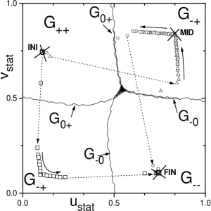
(a)

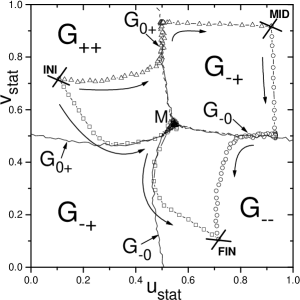
(b)

Figure 11: Stationary densities of right and left-movers $(u_{stat},v_{stat})\equiv\rho_{stat}$ for bidirectional traffic model from Monte Carlo simulations for a system with $300$ sites, along various Ph1 paths (Panel (a)) and Ph2 paths (Panel (b)). Reference Initial, Middle and Final points are marked by crosses INI, MID and FIN). Lines where one characteristic velocity is zero ($G_{0+},G_{-0}$) are obtained numerically. Evolution of the $\rho_{stat}(s)$ along a path is marked by arrows, dotted arrows mark discontinuous transitions. Few data points outside the arrow-marked paths result from finite size effects. The symmetry of the Figure with respect to the line $y=x$ is due to the left-right symmetry of the model and the points INI, FIN . Parameters: $h=0.5$. Panel (a): Squares mark $\rho_{stat}$ along a Ph1 path which goes directly from the initial to the final point INI$\rightarrow$ FIN. Triangles and circles mark $\rho_{stat}$ along two consecutive Ph1 paths INI$\rightarrow$ MID, MID$\rightarrow$ FIN. Initial, Middle and Final boundary rates, corresponding to points INI,MID,FIN are $(\alpha=1-\beta=0.1,A=1-B=0.78)$; $(\alpha=1-\beta=A=1-B=0.9)$ and $(A=1-B=0.1,\alpha=1-\beta=0.78)$. Along all paths, the boundary rates $\alpha,\beta,A,B$ are changed by linear interpolation law. Panel (b): The same as Panel (a), for respective Ph2 paths. Note that the densities along the direct Ph2 path (squares) go through the weak hyperbolic point $c_{1}=c_{2}=0$, marked by $M$, see also discussion at the end of Sec.VII. Initial,Middle and Final boundary rates: ($\alpha=1-\beta=0.1,A=1-B=0.75$), $(\alpha=1-\beta=A=1-B=0.95)$, and $(A=1-B=0.1,\alpha=1-\beta=0.75)$ respectively.

By computing the characteristic velocities along the path in physical region $\rho_{stat}(s)$ for $K=3$ we find that across each discontinuous transition just one characteristic velocity changes sign, this confirming the first-order phase transition scenario described in Sec. V.

Similarly, a single Ph2 path from initial to final state which belong to disjoint $G$ regions allows to observe the sequence of all continuous transitions between these states. As examples, see Figs. 9, 10 (see also the path marked by squares in Fig.11(b) of the next section for a more complex model). Note that it is important that that the initial state has more positive characteristic speeds than the final state.

ii) Fully matching path.

Another special path is a path where left and right boundary densities are equal all along from the initial till the end path point. It is clear that in this case we will not observe any phase transitions because there will be always a perfect match of the bulk density with the boundaries. Consequently, this path in parameter space must contain all triple points where the hyperplanes of second order and first order transitions merge together. For $K=1$ such a triple point is a point ($\rho^{\ast},\rho^{\ast}$) where the characteristic speed vanishes $j^{\prime}(\rho^{\ast})=0$. The nature and topology of the parameter space in vicinity of these triple points (lines, hypersurfaces) will be discussed elsewhere.

VIII Model for a bidirectional traffic on a narrow road

In the previous sections we concentrated our attention on solvable models with analytic flux functions and strict hyperbolicity. For generic (not integrable) models, however, the analytic flux function is typically unknown, as well as  exact relation between boundary rates and effective reservoir boundary densities. In the following we show how even in this case it is still possible to construct Ph1-like or Ph2-like paths along which a given BDPT type (discontinuous or continuous) can be observed. As an example, we consider the case of a two-way traffic model on a narrow road (see bottom panel of Fig. 3).

Models of bidirectional traffic have been widely studied in the literature and appear in several contexts see e.g. Juhasz (2010). Our system consists of two chains, containing particles hopping in opposite direction: a particle hops in preferred direction with constant rate $1$ and hard core exclusion like in TASEP, but is slowing down when it meets an upcoming particle (an obstacle) in front on the adjacent lane: in this case the rate of hopping is $\exp(-h)$, where a positive constant $h$ measures the interlane interaction, see Fig.3. A similar model, but with periodic boundary conditions, was considered in Jiang et al. (2009). We choose the boundary rates as follows: if the target site is vacant, a right-moving particle can enter with rate $\alpha$ ($\alpha e^{-h}$) if the adjacent to the target site is empty (is occupied by an upcoming particle). At the other end, a particle can leave with rate $\beta$. For the left moving particles, the entrance and exit rates are respectively $A$($Ae^{-h}$) and $B$. Note, that the model has the left-right symmetry. Since the model is not solvable, the analytical expression for the flux $j(u,v,h)$ is not known for any nonzero $h$. Neither we know the exact relation between the boundary rates and the effective boundary densities.

Ph1- and Ph2-like paths, however, can be constructed straightforwardly. From the physical meaning of the characteristic velocities (e.g. velocities with which small perturbations of the homogeneous state propagate) Popkov and Schütz (2003) we conclude that a stationary state with small density of right moving particles or right moving holes realized e.g. for $\alpha=1-\beta\ll 1$ and $B=1-A\ll 1$, has all positive characteristic velocities and therefore it must be in the $G_{++}$ region. By left-right symmetry, a stationary state with small density of left moving particles or holes will belong to the $G_{--}$ region ( the respective boundary rates are attainable from $G_{++}$ rates by exchanging $\alpha\Longleftrightarrow A,\beta\Longleftrightarrow B$). Finally, a state with small density of right movers on one lane and small density of left movers on another lane, realized by $\alpha,A,1-\beta,1-B\ll 1$ or $1-\alpha,1-A,\beta,B\ll 1$, belongs the $G_{-+}$ region. Proceeding along Ph1 (Ph2) paths in parameter space between regions $G_{++}\rightarrow$ $G_{-+}$, and $G_{-+}\rightarrow G_{--}$, one expects to see the occurrence of first (second) order phase transitions as described above. This is precisely what we obtain from Monte Carlo simulations of the two-way model, see Fig.11.

We can also build direct Ph1 and Ph2 paths between $G_{++}\rightarrow$ $G_{--}$ as described in Sec.VII i, see square data points in Fig.11. Note that along a direct Ph2 path (see Fig.11(b)), the pinning/depinning of stationary densities to the line with $c_{p}=0$ occurs only once, due to a presence of a special point (or region) $M$ in the middle where the lines $c_{1}=0$ and $c_{2}=0$ intersect. Such a point where two characteristic velocities coincide (the so- called weakly hyperbolic point), makes possible a continuous passage from $G_{++}$ to $G_{--}$ domain. It is worth to note that according to the numerical study of Jiang et al. Jiang et al. (2009) restricted to the case of periodic boundary conditions and equal particle densities, the steady state current along the symmetric line $u_{stat}=v_{stat}$ develops a plateau, leading in periodic system to phase separation. Such a non-analiticity in the stationary current suggests that the region $M$ in the middle of Fig.11(b) is a segment rather that a single point.

It is quite remarkable that even in this, rather special situation with non-analytic current-density dependence, our predictions about discontinuity/continuity of phase transitions along Ph1/Ph2 paths remain robust. We also remark that the presence of the region M can be neglected as long as our paths are situated far enough from it. The systematic study of an influence of a weakly hyperbolic point on BDPTs will be done elsewhere.

IX Conclusions

In this paper we have classified the basic phase transitions which can be observed in multi-species driven systems with open boundaries. We have shown that the splitting of the physical region into domains with different signs of characteristic speeds, and hyper-surfaces separating these regions where one of characteristic speeds vanishes, plays a fundamental role in this classification. Adiabatic paths in the parameter space, defined by the particle densities of each specie at the left and right boundary reservoirs, along which we surely observe discontinuous or continuous transition of a desired type, or a desired sequence of BDPTs, have been explicitly constructed. The details of the microscopic dynamics and the geometry of the models are not important for our qualitative BDPTs scenarios to occur, as far as several conditions listed at the beginning of Sec.II are fulfilled. We expect therefore our results to be valid for a broad class of particle models with several interacting particle species. In particular, our examples were systems of particles obeying hard-core exclusion rule, but this is not required as far as some interaction making the flux function nonlinear will be present.

Mathematically, our study has been focused mainly to models with analytic flux function and strict hyperbolicity i.e. models with Jacobian matrices which have distinct eigenvalues in all the physical region. An example of a weakly hyperbolic model with non-analytic flux and phase separation, however, was considered in Sec.VIII. It is remarkable that even for this model the general validity of our approach has been confirmed. An interesting problem for the future would be to test the predictions of our analysis on more complicated models, like those showing symmetry breaking, hysteresis and ergodicity breaking phenomena.

X Acknowledments

It is a pleasure to thank G. Schütz for discussion and valuable comments. VP wish to thank the Department of Physics and the University of Salerno, for hospitality and for providing a research grant (Assegno di Ricerca no. 1508, 2007-2010) during which this work was done. This work has been partially supported by the DFG grant 436 RUS 113/909/0-1(R) and by the Italian Ministry for Education, University and Research (MIUR) through an inter-University PRIN-2008 initiative.

References

- (1)
- (2)
- (3)
- (4)
- (5)
- Gunter (03) G. Schütz, J. Phys. A 36, R339 (2003).
- KoloFischer (2007) A.B. Kolomeisky and M.E. Fisher, Annu. Rev. Phys. Chem. 58, 675 (2007).
- (8) A. Basu and E. Frey, J. Stat. Mech. , p. P09013 (2009).
- Krug (1991) J. Krug, Phys. Rev. Lett. 67, 1882 (1991).
- Kolomeisky et al. (1998) A. B. Kolomeisky, G. M. Schütz, E. B. Kolomeisky, and J. P. Straley, J. Phys. A 31, 6911 (1998).
- Popkov (2007) V. Popkov, Journal of Stat. Mechanics: Theory and Experiment p. P07003 (2007).
- Lax (1973) P. D. Lax, Hyperbolic Systems of Conservation Laws and the Mathematical Theory of Shock Waves (SIAM series, Philadelphia, vol. 11, 1973).
- Lax (2006) P. D. Lax, Hyperbolic Partial Differential Equations (Courant Lecture Notes in Mathematics, vol. 14, New York, 2006).
- Bressan (2000) A. Bressan, Hyperbolic Systems of Conservation Laws (Oxford University Press, New York, 2000).
- Popkov and Schütz (1999) V. Popkov and G. M. Schütz, Europhys. Lett 48, 257 (1999).
- Popkov and Schütz (2004) V. Popkov and G. M. Schütz, J.Stat. Mech.:Theory and Experiment p. P12004 (2004).
- (17) For some models, the characteristic velocities may coincide at certain parameter values. This leads in the hydrodynamic limit to weakly hyperbolic equations, and extra phenomena, see e.g. Popkov and Peschel (2001). Here we focus on models with strict hyperbolicity, where the characteristic velocities are always distinct.
- Popkov and Schütz (2003) V. Popkov and G. M. Schütz, J Stat. Phys. 112, 523 (2003).
- Schütz (2000) G. M. Schütz, Exactly solvable models for many-body systems far from equilibrium (Academic Press, London, 2000), in: Phase Transitions and Critical Phenomena, ed. C.Domb and J.L. Lebowitz, Vol. 19.
- Derrida (1998) B. Derrida, Physics Reports 301, 65 (1998).
- Popkov and Salerno (2004) V. Popkov and M. Salerno, Phys. Rev. E 69, 046103 (2004).
- Popkov (2004) V. Popkov, J. Phys. A 37, 1545 (2004).
- Juhasz (2010) R. Juhasz, J Stat Mech p. P03010 (2010).
- Jiang et al. (2009) R. Jiang, K. Nishinari, M. B. Hu, Y. H. Wu, and Q. S. Wu, J Stat Phys 136, 73 (2009).
- Popkov and Peschel (2001) V. Popkov and I. Peschel, Phys. Rev. E 64, 026126 (2001).