FLUID SIMULATIONS WITH LOCALIZED BOLTZMANN UPSCALING BY DIRECT SIMULATION MONTE-CARLO

Abstract

In the present work, we present a novel numerical algorithm to couple the Direct Simulation Monte Carlo method (DSMC) for the solution of the Boltzmann equation with a finite volume like method for the solution of the Euler equations. Recently we presented in [14],[16],[17] different methodologies which permit to solve fluid dynamics problems with localized regions of departure from thermodynamical equilibrium. The methods rely on the introduction of buffer zones which realize a smooth transition between the kinetic and the fluid regions. In this paper we extend the idea of buffer zones and dynamic coupling to the case of the Monte Carlo methods. To facilitate the coupling and avoid the onset of spurious oscillations in the fluid regions which are consequences of the coupling with a stochastic numerical scheme, we use a new technique which permits to reduce the variance of the particle methods [11]. In addition, the use of this method permits to obtain estimations of the breakdowns of the fluid models less affected by fluctuations and consequently to reduce the kinetic regions and optimize the coupling. In the last part of the paper several numerical examples are presented to validate the method and measure its computational performances.

Keywords: Kinetic-fluid coupling, Boltzmann equation, multiscale problems, Monte Carlo methods.
AMS Subject classification: 65M55, 76P05, 82B05, 82C80

1 Introduction

Many problems of interests in applications involve non equilibrium gas flows as hypersonic objects simulations or micro-electro-mechanical devices. Often, these kinds of problems are characterized by breakdowns of fluid models, either Euler or Navier-Stokes. Now, when the breakdown is localized both in space and time we must deal with conjunctions of continuum and non equilibrium regions. To face such problems, the most natural approach is to try to combine numerical schemes for continuum models with microscopic kinetic models which guarantee a more accurate description of the physics when far from thermodynamical equilibrium conditions are reached. In fact, it is not always necessary to solve the Boltzmann equation, which is computationally more expensive by several orders of magnitude than a continuum description, in the entire domain. It is, instead, sufficient to use the microscopic description in regions where the departure from equilibrium is strong and manifests itself as boundary layers or shocks.

The construction of such hybrid kinetic-fluid methods involve three main problems. The first one is how to accurately identify the different regions. We refer, for instance, to the works of Wijesinghe and Hadjiconstantinou [35], Levermore, Morokoff, and Nadiga [22], and Wang and Boyd [31], in which various breakdown criteria are analyzed and then proposed. The second main problem is how to, in practice, realize the coupling. In other words, how to match the two models at the interfaces. Several different ideas are described in the works of Bourgat, LeTallec, Perthame, and Qiu [4], Bourgat, LeTallec and Tidriri [5], LeTallec and Mallinger [23], Aktas and Aluru [1], Roveda, Goldstein and Varghese [25, 26], Sun, Boyd and Candler [7, 32], Wadsworth and Erwin [34]. Domain decomposition approaches are also popular in others fields such as, for instance in epitaxial growth [27] or for problems involving different scaling such as the diffusive scalings [13, 20]. The decomposition between equilibrium and non equilibrium states can be realized also in the velocity space instead of physical space [10], [18]. It is important to stress that most of the mentioned methods use a static interface between kinetic and fluid regions. However, this approach appears as somehow inadequate and inefficient for many realistic problems. To overcome this difficulty, automatic domain decomposition methods have also been developed in the recent past. See for example Kolobov et al. [21], or Tiwari [29, 30] and Degond, Dimarco and Mieussens [16, 17]. The third problem is the choice of the appropriate numerical methods for solving the macroscopic and the microscopic model. A first possibility are the deterministic-deterministic methods in which both the macroscopic and the microscopic models are solved by means of finite volume techniques such as for instance in [14, 16, 17]. These methods permit to obtain very accurate results but generally they are too expensive. For this reason simplified models are then used to describe the kinetic part of the problem. In practice, in most of the cases, the collision operator is replaced by the BGK relaxation operator which permits to reduce the computational cost. A second approach consists in using particle-particle methods [28, 7]. These methods avoid the complexity associated with using two independent methods for different regions and provide a simple solution to the interface problem. On the other hand, the solutions contain large statistical errors which are the typical drawback of Monte Carlo methods. Recently, some low diffusion particle-particle numerical methods have been proposed by Boyd and coauthors in [6]. A third approach is the deterministic- particle approach [33, 34, 36, 19, 32]. Here, the fluid model is discretized by using a finite volume method, while the kinetic model is solved by the DSMC method. The popularity of DSMC is due to several advantages compared to other simulation methods for kinetic equations, including advantages related to efficiency, memory usage and implementation of additional physical phenomena. The disadvantages of DSMC, however, are the increase of the computational cost close to thermodynamical equilibrium and the large statistical error which scales with the inverse square root of the number of particles. This last aspect is the cause of the big difficulties met in the coupling, both for defining the kinetic regions and to avoid the introduction of oscillations in the fluid part.

In the present paper, we present a novel numerical algorithm to couple a DSMC method for the solution of the Boltzmann model and a finite volume like method for the Euler equations. The method relies on two main aspects. The first one is the use of a new low variance Direct Simulation Monte Carlo method to compute the solution of the kinetic part. Monte Carlo methods, as already observed, permit more realistic descriptions of the physical problems. On the other hand, the solutions computed with these techniques are affected by large statistical noise. In order to reduce this effect, we extend the variance reduction technique (called moment guided method) which has been recently developed in [12] to the coupling case. The moment guided method permits to reduce the statistical error through a matching with a set of suitable macroscopic moment equations. The basic idea, on which the method relies, consists in guiding the particle positions and velocities through moment equations so that the concurrent solution of the moment and kinetic models furnishes the same macroscopic quantities. The method is based on the observation that the deterministic solution of the moment equation leads to a more accurate solution, in term of statistical fluctuations, than the DSMC method. We experimentally showed in [11] that this is indeed the case. Now, a crucial point, in the implementation of the domain decomposition strategies, is the identification of the zones in which the microscopic description is necessary. In other words, kinetic regions have to be as thin as possible, with the constraint that the effective solution is correctly captured. Thus, the direct consequence of using the moment guided method to solve the Boltzmann equation is that the research of the interface location becomes a less difficult task to accomplish. Moreover, the use of this technique permits to reduce significantly the propagation of spurious oscillations in the fluid regions.

The second main aspect of the method consists of the introduction of a buffer zone which realizes a smooth transition between the kinetic and fluid regions. It differs from the method of [14, 15, 16, 17] by the way the solution of the Boltzmann equation is decomposed into a kinetic and a fluid component. The new decomposition we adopt is better adapted to a DSMC method while the earlier one was more adapted to grid based solutions of the Boltzmann equation. As in [11], we suggest a methodology to allow for the time evolution of the kinetic and fluid regions which permits to follow discontinuities in time and space and solve the microscopic model only where necessary. Thanks to this technique, it is possible to achieve considerable computational speedup compared with steady interface coupling strategies, without otherwise, losing accuracy in the solution. Finally, we observe that the use of a smooth transition between the micro and the macro models further reduces the propagation of fluctuations in the fluid regions and thus it permits to obtain more accurate results.

The outline of the article is the following. In section 2, we introduce the Boltzmann equation, its properties and the fluid limit. In section 3 we describe the moment guided method while in section 4 we present the coupling strategy. Section 5 is devoted to the discretization of the Boltzmann equation and of the finite volume scheme for the Euler equations. In section 6, we describe the breakdown criterion. Several numerical tests are presented in section 7 to illustrate the properties of our method and to demonstrate its efficiency in comparison with DSMC schemes. A short conclusion is given in section 8.

2 The Boltzmann equation and its fluid limit

We consider the following model [9]

$$\partial_{t}f+v\cdot\nabla_{x}f=Q(f,f),$$ (1)

with the initial data

$$f(x,v,t=0)=f_{0},$$

where $f=f(x,v,t)$ is the density of particles that have velocity $v\in{}^{3}$ and position $x\in\Omega\subset{}^{3}$ at time $t>0$. The collision operator $Q$ locally acts in space and time and takes into account interactions between particles. It is written:

$$Q(f,f)=\int_{{}^{3}}\int_{S^{2}}B\left(|q|,\frac{q\cdot n}{|q|}\right)[f(v^{\prime})f(v^{\prime}_{*})-f(v)f(v_{*})]dndv_{*}.$$ (2)

In the above expression $S^{2}$ is the unit sphere in ³, $q=v-v_{*}$ the relative velocity, $n\in S^{2}$ the unit vector in the direction of the scattered velocity. The collision kernel $B(|q|,q\cdot n/|q|)$ characterizes the detail of the collision and is defined as

$$B(|q|,\cos\theta)=|q|\sigma(|q|,\theta),\ (0\leq\theta\leq\pi)$$ (3)

where $\cos\theta=q\cdot n/|q|$ and $\sigma(|q|,\theta)$ is the collision cross section which corresponds to the scattering angle $\theta$. Finally the post collisional velocity are computed by

$$v^{\prime}=\frac{1}{2}(v+v_{*}+|q|n),\ v^{\prime}_{*}=\frac{1}{2}(v+v_{*}-|q|n).$$ (4)

The collisional operator locally satisfies the conservation of mass, momentum and energy:

$$\langle mQ(f,f)\rangle=0$$ (5)

for every $f$, where we denote weighted integrals of $f$ over the velocity space by

$$\langle\phi f\rangle=\int_{{}^{3}}\phi(v)f(v)dv,$$ (6)

with $\phi(v)$ any function of $v$, and $m(v)=(1,v,|v|^{2})$ are the collisional invariants. The multiplication of (1) by $m(v)$ and the integration in velocity space leads to the following system of local conservation laws

$$\partial_{t}\langle mf\rangle+\nabla_{x}\cdot\langle vmf\rangle=0.$$ (7)

Now, the well known Boltzmann s H-theorem implies that any equilibrium distribution function, i.e. any function $f$ for which $Q(f,f)=0$, has the form of a locally Maxwellian distribution:

$$E[\boldsymbol{\varrho]}(v)=\frac{\varrho}{(2\pi\theta)^{3/2}}\exp\left(\frac{-|u-v|^{2}}{2\theta}\right),$$ (8)

where $\boldsymbol{\varrho}=(\varrho,\varrho u,\varrho e)$, with $\varrho$ and $u$ the density and mean velocity while $\theta=RT$, with $T$ the temperature of the gas and $R$ the gas constant. The macroscopic values $\varrho$, $u$ and $T$ are related to $f$ by:

$$\varrho=\int_{{}^{3}}fdv,\qquad\varrho u=\int_{{}^{3}}vfdv,\qquad\theta=\frac{1}{3\varrho}\int_{{}^{3}}|v-u|^{2}fdv,$$ (9)

while the fluid energy $e$ is defined as

$$e=\frac{1}{2\varrho}\int_{{}^{3}}|v|^{2}fdv=\frac{1}{2}|u|^{2}+\frac{3}{2}\theta.$$ (10)

When the mean free path between particles is very small compared to the size of the computational domain, the space and time variables can be rescaled to

$$x^{\prime}=\varepsilon x,\ t^{\prime}=\varepsilon t$$ (11)

where $\varepsilon$ is the ratio between the microscopic and the macroscopic scale (the so-called Knudsen number). Using these new variables in (1), we get

$$\partial_{t^{\prime}}f^{\varepsilon}+v\cdot\nabla_{x^{\prime}}f^{\varepsilon}=\frac{1}{\varepsilon}Q(f^{\varepsilon},f^{\varepsilon}).$$ (12)

If the Knudsen number $\varepsilon$ tends to zero, formally the distribution function converges towards the local Maxwellian equilibrium $E^{\varepsilon}[\boldsymbol{\varrho}]$. Inserting this relation into the conservation laws (7) gives the set of compressible Euler equations for the macroscopic quantities $\boldsymbol{\varrho}$:

$$\partial_{t^{\prime}}\boldsymbol{\varrho}+\nabla_{x^{\prime}}\cdot F(\boldsymbol{\varrho})=0,$$ (13)

where $F(\boldsymbol{\varrho})=\langle vmE^{\varepsilon}[\boldsymbol{\varrho}]\rangle$.

In the sequel we will omit the primes to simplify notations wherever they will not cause in confusion.

3 The moment guided method

In this section we introduce the method which permits to reduce statistical fluctuations in the DSMC scheme. We refer to [11, 12] for details on the method. The starting point of the moment guided method consists in decomposing the distribution function $f$ as a part in equilibrium and a part in non equilibrium. We call this decomposition micro-macro decomposition

$$f=E[\boldsymbol{\varrho}]+g.$$ (14)

The function $g$ represents the non-equilibrium part of the distribution function. From the definition above, it follows that $g$ is in general non positive. Moreover since $f$ and $E[\boldsymbol{\varrho}]$ have the same moments we have

$$\langle m(v)g\rangle=0.$$ (15)

Finally, it is possible to show that $E[\boldsymbol{\varrho}]$ and $g$ satisfy the following coupled system of equations

$$\partial_{t}\boldsymbol{\varrho}+\nabla_{x}\cdot F(\boldsymbol{\varrho})+\nabla_{x}\cdot\langle vm(v)g\rangle=0,$$ (16)

$$\partial_{t}f+v\cdot\nabla_{x}f=\frac{1}{\varepsilon}Q(f,f)$$ (17)

We skip the proof of the above statement and we refer to [15] for details on the micro-macro decomposition and its properties.

The idea of the moment guided strategy is to solve the kinetic equation (17) with the Monte Carlo method, and concurrently the fluid equation with a finite volume scheme. The correction term which is necessary to close the macroscopic equations $\nabla_{x}\cdot\langle vm(v)g\rangle$ is evaluated using particle moments. We observe that the two equations (16-17), except for numerical errors, give the same results in terms of macroscopic quantities. We assume that the set of moments obtained from the fluid system represents a better statistical estimate of the true moments of the solution, since the resolution of the moment equations does not involve any stochastic process. We experimentally showed that this is the case in [11].

Consider a time discretization of the problem (16-17), then the method is summarized in the following steps: at each time step $t^{n}$

1. Solve the kinetic equation (17) with any type of DSMC method and obtain a first set of moments.

2. Solve the fluid equation (16) with any type of finite volume scheme where particles are used to evaluate $\nabla_{x}\cdot\langle vm(v)g\rangle$ and obtain a second set of moments.

3. Match the moments of the kinetic solution with the fluid solution through a transformation of the samples values.

4. Restart the computation to the next time step.

In the following we will consider the case in which the perturbation $g$ is very small in a part of the domain while it is large in the complementary part. In the small perturbation regions it will be suitable to avoid the solution of the kinetic equation (17) and solve only the Euler equations which are able to furnish an accurate description of the problem under consideration. However, the direct passage from the micro to the macro model does not prevent the fluctuations, which has been reduced with the moment guided method but which are not completely disappeared, to propagate to the fluid regions. In order to avoid this loss of accuracy, we introduce in the next section a model which realizes a smooth transition between the different regions.

4 The coupling method

Let $\Omega_{1}$, $\Omega_{2}$, and $\Omega_{3}$ be three disjointed sets such that $\Omega_{1}\cup\Omega_{2}\cup\Omega_{3}={}^{3}$. The first set $\Omega_{1}$ is supposed to be a domain in which the flow is far from the equilibrium (the ”kinetic zone”, $g$ large), while the flow is supposed to be close to equilibrium in $\Omega_{2}$ (the ”fluid zone”, $g\simeq 0$). The third region is the buffer zone and also in $\Omega_{3}$ we suppose the gas to be close to thermodynamical equilibrium. We define a function $h(x,t)$ such that

$$h(x,t)=\left\{\begin{array}[]{lll}\displaystyle 1,&\mbox{for}&x\in\Omega_{1},\\ 0,&\mbox{for}&x\in\Omega_{2},\\ 0\leq h(x,t)\leq 1,&\mbox{for}&x\in\Omega_{3}.\\ \end{array}\right.$$ (18)

Note that the time dependence of $h$ means that we account for dynamically changing the shape of the transition function. The topology and geometry of the different zones is directly encoded in $h$ and may change dynamically as well.

Multiplying (17) by $h$ and $1-h$, we get

$$\partial_{t}\boldsymbol{\varrho}+\nabla_{x}\cdot F(\boldsymbol{\varrho})+\nabla_{x}\cdot\langle hvm(v)g\rangle+\nabla_{x}\cdot\langle(1-h)vm(v)g\rangle=0,$$ (19)

$$\partial_{t}(hf)+v\cdot\nabla_{x}(hf)=\frac{h}{\varepsilon}Q(f,f)+\left(\frac{\partial_{t}h}{h}+v\cdot\frac{\nabla_{x}h}{h}\right)(hf),$$ (20)

$$\partial_{t}((1-h)f)+v\cdot\nabla_{x}((1-h)f)=\frac{1-h}{\varepsilon}Q(f,f)-\left(\frac{\partial_{t}h}{h}+v\cdot\frac{\nabla_{x}h}{h}\right)(hf).$$ (21)

Denoting $f_{K}=hf$, $f_{F}=(1-h)f$, $g_{K}=hg$ and $g_{F}=(1-h)g$ the ensemble $(f_{K},f_{F},\boldsymbol{\varrho},g_{K},g_{F})$ satisfies the system

$$\partial_{t}\boldsymbol{\varrho}+\nabla_{x}\cdot F(\boldsymbol{\varrho})+\nabla_{x}\cdot\langle vm(v)g_{K}\rangle+\nabla_{x}\cdot\langle vm(v)g_{F}\rangle=0,$$ (22)

$$\partial_{t}f_{K}+v\cdot\nabla_{x}f_{K}=\frac{h}{\varepsilon}Q(f_{K}+f_{F},f_{K}+f_{F})+\left(\frac{\partial_{t}h+v\cdot\nabla_{x}h}{h}\right)f_{K},$$ (23)

$$\partial_{t}f_{F}+v\cdot\nabla_{x}f_{F}=\frac{1-h}{\varepsilon}Q(f_{K}+f_{F},f_{K}+f_{F})-\left(\frac{\partial_{t}h+v\cdot\nabla_{x}h}{h}\right)f_{K},$$ (24)

We observe that the system (22)-(24) is equivalent to equation (1) in the sense that if $f$ is a solution of (1) with initial datum $f(t=0)=f_{0},\ g(t=0)=g_{0}=f(t=0)-E[\boldsymbol{\varrho}(t=0)]$ then $f_{K}=hf$, $f_{F}=(1-h)f$, $g_{K}=hg$, $g_{F}=(1-h)g$ and $\boldsymbol{\varrho}=\langle m(v)f\rangle$ are solutions of system (22)-(24) with initial data $f_{K}(t=0)=hf_{0}$, $f_{F}(t=0)=(1-h)f_{0}$, $g_{K}(t=0)=hg_{0}$, $g_{F}(t=0)=(1-h)g_{0}$ $\boldsymbol{\varrho}(t=0)=\langle m(v)f_{0}\rangle$. Reciprocally, if $f_{K}$, $f_{F}$, $g_{K}$, $g_{F}$ and $\boldsymbol{\varrho}$ are solutions of (22)-(24) with initial data $f_{K}(t=0)=hf_{0}$, $f_{F}(t=0)=(1-h)f_{0}$, $g_{K}=hg_{0}$, $g_{F}=(1-h)g_{0}$ and $\boldsymbol{\varrho}(t=0)=\langle m(v)f_{0}\rangle$ then $f=f_{K}+f_{F},\ g=g_{K}+g_{F}=f-E[\boldsymbol{\varrho}]$ is the solution of (1) with initial data $f(t=0)=f_{0}$ and $g(t=0)=g_{0}$.

Now assume that the flow is very close to equilibrium in $\Omega_{2}\cup\Omega_{3}$. This means that we assume the distribution function to be Maxwellian in this set: $f_{F}=E[\boldsymbol{\varrho}_{F}]$ and thus $g_{F}=0$. Then, equation (24) can be eliminated and we get:

$$\partial_{t}\boldsymbol{\varrho}+\nabla_{x}\cdot F(\boldsymbol{\varrho})+\nabla_{x}\cdot\langle vm(v)g_{K}\rangle=0,$$ (25)

$$\partial_{t}f_{K}+v\cdot\nabla_{x}f_{K}=\frac{h}{\varepsilon}Q(f_{K}+E[\boldsymbol{\varrho}_{F}],f_{K}+E[\boldsymbol{\varrho}_{F}])+\left(\frac{\partial_{t}h+v\cdot\nabla_{x}h}{h}\right)f_{K}.$$ (26)

System (25–26) represents our kinetic-fluid model. In this model the local distribution function $f$ is approximated by $E[\boldsymbol{\varrho}]+g_{K}$ where $g_{K}=f_{K}-E[\boldsymbol{\varrho}_{K}]$. The distribution $E[\boldsymbol{\varrho}_{K}]$ is defined as the Maxwellian whose moments are given by $\langle m(v)f_{K}\rangle$, while $E[\boldsymbol{\varrho}_{F}]$ is the Maxwellian whose moments are given by $\boldsymbol{\varrho}-\langle m(v)f_{K}\rangle$. Observe that $f_{K}$ is zero in the fluid zone $\Omega_{2}$ as well as $g_{K}$. This means that, in these regions, we simply solve the compressible Euler equations. On the other hand, in $\Omega_{1}$ the function $\langle m(v)f_{K}\rangle=\boldsymbol{\varrho}$ and thus the system (25–26) reduces to the system (16–17) which is equivalent to the Boltzmann equation (1) where we employ the moment guided method to reduce the variance of the DSMC method.

In the next section we will discuss the numerical scheme which discretizes the system (25–26) as well as the boundary conditions between the different regions.

5 The numerical schemes

5.1 The DSMC method for the coupled Boltzmann equation

The classical approach used to solve the Boltzmann equation by Monte Carlo methods is the time splitting approach [2, 24] between the free transport term

$$\partial_{t}f_{K}+v\cdot\nabla_{x}f_{K}=0,$$ (27)

and the collision term

$$\partial_{t}f_{K}=\frac{h}{\varepsilon}Q(f_{K}+E[\boldsymbol{\varrho}_{F}],f_{K}+E[\boldsymbol{\varrho}_{F}]).$$ (28)

We start to discuss the discretization of the transport term which, in our model, is replaced by the free transport term plus the term which involves the time and space derivative of the transition function $h$ ($h$-term).

5.1.1 Free transport step

We introduce a space discretization of mesh size $\Delta x$ and a time discretization of time step $\Delta t$. The discretization of the domain is not needed for the transport step which is solved exactly for particles but it is necessary to solve the collision part of the problem which acts locally in space and thus it is necessary to solve the full problem. In Monte Carlo simulations the distribution function $f_{K}$ is discretized by a finite set of particles

$$f_{K}=\frac{m_{p}}{N}\sum_{i=1}^{N}\alpha_{i}(t)\,\delta(x-X_{i}(t))\delta(v-V_{i}(t)),$$ (29)

where $X_{i}(t)$ represents the particle position in the three spatial directions, $V_{i}(t)$ the particle velocities in the velocity space, $m_{p}$ a constant and $\alpha_{i}(t)$ the weight to associate to each particle. During the transport step (27), the particles move to their next positions according to

$$X_{i}(t+\Delta t)=X_{i}(t)+V_{i}(t)\Delta t$$ (30)

where (29) with (30) and $\alpha_{i}=1$ represents an exact solution of equation (27). On the other hand, an exact solution of the modified transport equation

$$\partial_{t}f_{K}+v\cdot\nabla_{x}f_{K}=\left(\frac{\partial_{t}h+v\cdot\nabla_{x}h}{h}\right)f_{K}$$ (31)

is a distribution of the form (29) if $X_{i}(t)$ and $\alpha_{i}(t)$ satisfy the system

$$\dot{X}_{i}=V_{i}\,,$$ (32)

$$\alpha_{i}(t)=h(X_{i},t).$$ (33)

This can be shown by inserting (29) inside (31). The previous solution of equation (31) holds for all choices of $V_{i}$. The transition function $h$ is discretized on the mesh of size $\Delta x$ and thus particles which belongs to the same cell have the same weight. These relations mean that the weights vanish in the buffer zone proportionally to the local value of $h$. Consequently, at the boundary of the buffer zones on the fluid side, the particles are weightless and can be removed. Simultaneously, the velocity is not affected by the value of the cut-off function (as for instance in the decomposition used in [14] and [16]), which means that there is no accumulation of weightless particles at the boundaries.

Thus, the Monte Carlo solution of the transport step consists in moving the particles in space according to equation (30) as in the classical transport case. The only difference is that the mass of each particle changes in time and space according to the transition function value $h$ and it takes values between $0$ when $h(x,t)=0$ (which means in cells in which the gas is in thermodynamical equilibrium) and $m_{p}$ when $h(x,t)=1$ (which means in the cells in which the gas is far from equilibrium). The constant $m_{p}$ is defined at the beginning of the computation in the following way

$$m_{p}=\frac{1}{N}\int_{\Omega}\int_{{}^{3}}f_{K}(t=0)dvdx.$$ (34)

Thus, the transport step is composed of two substeps: transport of particles and mass rescaling. Finally, to guarantee preservation of macroscopic quantities we need boundary conditions. This means we need to inject weightless particles at the boundaries of the buffer zones on the fluid sides. The gas, being in thermodynamical equilibrium in these regions, we just sample the number of requested particles from a Maxwellian distribution whose associated macroscopic quantities are the ones given by the solution of the fluid model.

5.1.2 The moment matching

We discuss now the matching method between the kinetic equation and the macroscopic equations. Imagine that the value of the macroscopic moments $\boldsymbol{\varrho}^{n+1}$ obtained from the solution of system (25) is known at time $n+1$. Now, in the kinetic regions we want to match these moments with the moments $\widetilde{\boldsymbol{\varrho}}_{K}^{n+1}$ obtained solving the transport part of the kinetic equation (31). On the other hand, in buffer regions, the mass of particles decreases linearly with the transition function $h$. This means that the matching has to be done between $h\boldsymbol{\varrho}^{n+1}$ and $\widetilde{\boldsymbol{\varrho}}_{K}^{n+1}$, where when $h=1$ we have the matching between the macroscopic equations and the Boltzmann equation and when $h=0$ we do not perform any matching. Observe that, the collision step conserves the moments while it changes the shape of the distribution in velocity space. Thus $\widetilde{\boldsymbol{\varrho}}_{K}^{n+1}$ represents the moments solution obtained by solving the kinetic equation (26) at time $n+1$ independently of the type and number of collisions.

We first discuss the matching of momentum and energy which can be realized through the following linear transformation: let consider the set of velocities $V_{1},\ldots,V_{N_{\mathcal{I}_{j}}}$ inside the cell $\mathcal{I}_{j}$ at time $n+1$, where $N_{\mathcal{I}_{j}}$ is the number of particles inside the cell $j$. In the Monte Carlo setting the first two moments are given by

$$\mu_{1}=\frac{1}{N_{\mathcal{I}_{j}}}\sum_{i\in\mathcal{I}_{j}}^{N_{\mathcal{I}_{j}}}V_{i}\qquad\mu_{2}=\frac{1}{N_{\mathcal{I}_{j}}}\sum_{i\in\mathcal{I}_{j}}^{N_{\mathcal{I}_{j}}}\frac{1}{2}|V_{i}|^{2},$$ (35)

where $\mu_{1}$ is a vector representing the mean velocity in the three spatial directions. Suppose now that better estimates $\sigma_{1}$ and $\sigma_{2}$ of the same moments are available. They are, for instance, obtained by resolving the moment equations (25). We apply the transformation described in [8] and get velocities $V_{i}^{*}$ given by

$$V_{i}^{*}=(V_{i}-\mu_{1})/c+\sigma_{1}\quad c=\sqrt{\frac{\mu_{2}-\mu_{1}^{2}}{\sigma_{2}-\sigma_{1}^{2}}},\quad i=1,\ldots,\mathcal{I}_{j}$$ (36)

to get

$$\frac{1}{N_{\mathcal{I}_{j}}}\sum_{i\in\mathcal{I}_{j}}^{N_{\mathcal{I}_{j}}}V_{i}^{*}=\sigma_{1},\qquad\frac{1}{N_{\mathcal{I}_{j}}}\sum_{i\in\mathcal{I}_{j}}^{N_{\mathcal{I}_{j}}}\frac{1}{2}|V_{i}^{*}|^{2}=\sigma_{2}.$$

Let us now discuss the matching of the zero-th order moment: the mass density. In this case, we first observe that the above renormalization is not possible if we want to keep the mass of the particles constant and uniform inside the cells. We denote by $\mu_{0}$ an estimate of the zero-th order moment and by $\sigma_{0}$ its better evaluation obtained solving the moment equations (25). Among the possible techniques that can be used to restore a prescribed density, we choose to replicate or discard particles inside the cells. Other possibilities are discussed in [12].

In the discarding procedure case we eliminate the following number of particles:

$$\widetilde{N_{p}}=\mathop{\mbox{\rm Iround}}\nolimits\left(\frac{\mu_{0}-\sigma_{0}}{m_{p}}\right),$$ (37)

where $\mathop{\mbox{\rm Iround}}\nolimits$ represents a stochastic rounding. This means that a mismatch $e$ such that $e<\pm m_{p}$ is unavoidable when the mass of the particle is constant and uniform. Observe that, we already change, at each time step, the mass of the particles according to the transition function $h$. However, if we change the particles mass to match the density, this implies that, due to the transport step, we will end with particles of different weights in the same cells. This situation will cause difficulties for the collision step procedure that we want to avoid. In the case of change of mass due to the transition function, we do not have this problem, because particles which belong to the same cell have the same mass, $h$ being constant inside each cell.

In the opposite case, in which the mass of the particles inside a cell is lower than the mass prescribed by the fluid equations $\mu_{0}<\sigma_{0}$, the situation is less simple. Here, since the distribution function is not known analytically, it is not possible to sample new particles without introducing correlations between samples. In this case we replicate

$$\widetilde{N_{p}}=\mathop{\mbox{\rm Iround}}\nolimits\left(\frac{\sigma_{0}-\mu_{0}}{m_{p}}\right)$$ (38)

particles randomly with uniform probability. We then perform a stochastic rounding of $(\sigma_{0}-\mu_{0})/{m_{p}}$ by lower and upper values. Note that this replication is done allowing repetitions of the choice of the particle to replicate. After the generation step, samples are relocated uniformly inside each spatial cell.

5.1.3 Collision step

We consider now the solution of the collision step (28). The effect of this step is to change the shape of the velocity distribution and to project it towards the equilibrium distribution leaving unchanged mass momentum and energy. The collision operator acts locally in space which means that we solve it independently in each spatial cell where the particles are assumed to have all the same weight ($h$ is constant in each cell). The initial data of this step is given by the solution of the transport step after the moment matching procedure. We assume that the collision term (28) can be written in the form

$$\partial_{t}f_{K}=\frac{h}{\varepsilon}[P(f_{K}+E[\boldsymbol{\varrho}_{F}],f_{K}+E[\boldsymbol{\varrho}_{F}])-\mu(f_{K}+E[\boldsymbol{\varrho}_{F}])],$$ (39)

where $\mu>0$ is a constant which typically corresponds to an estimation of the largest spectrum of the loss part of the collision operator. The operator $P(f,f)$ is a non negative bilinear operator such that

$$\frac{1}{\mu}\int_{{}^{3}}P(f,f)(v)m(v)\,dv=\int_{{}^{3}}f(v)m(v)\,dv.$$ (40)

For example for Maxwellian molecules

$$P(f,f)=Q^{+}(f,f)(v)=\int_{\mathbb{R}^{3}}\int_{S^{2}}b_{0}(\cos\theta)f(v^{\prime})f(v_{\ast}^{\prime})\,d\omega\,dv_{\ast},$$ (41)

and $\mu=\varrho$. In the numerical tests presented in this paper, we considered Maxwellian molecules. In any case, the use of different and more general kernels does not involve any change in the coupling method. Now, since the assumption in our model is that the distribution $E[\boldsymbol{\varrho}_{F}]$ is Maxwellian and constant along the collision step, we can rewrite (39) in the following way:

$$\partial_{t}\left(f_{K}+E[\boldsymbol{\varrho}_{F}]\right)=\frac{h}{\varepsilon}[P(f_{K}+E[\boldsymbol{\varrho}_{F}],f_{K}+E[\boldsymbol{\varrho}_{F}])-\mu(f_{K}+E[\boldsymbol{\varrho}_{F}])],$$ (42)

Let now $f_{K,j}^{n*}(v)$ be an approximation of $f_{K}(v,n\Delta t,jx_{j})$ after transport and matching. The forward Euler scheme for equation (42) writes [24]

$$f_{K,j}^{n+1}+E[\boldsymbol{\varrho}_{F,j}^{n+1}]=\left(1-\frac{h\mu\Delta t}{\epsilon}\right)\left(f_{K,j}^{n*}+E[\boldsymbol{\varrho}_{F,j}^{n*}]\right)+\frac{h\mu\Delta t}{\epsilon}\frac{P(f_{K,j}^{n*}+E[\boldsymbol{\varrho}_{F,j}^{n*}],f_{K,j}^{n*}+E[\boldsymbol{\varrho}_{F,j}^{n*}])}{\mu}.$$ (43)

Observe that $E[\boldsymbol{\varrho}_{F,j}^{n+1}]=E[\boldsymbol{\varrho}_{F,j}^{n*}]$. This means that at the Monte Carlo level, the above formula can be interpreted in the following way: in order to obtain the statistical solution of the distribution function at time step $n+1$, $f^{n+1}_{K,j}$, we need to

• sample with probability $(1-{\mu\Delta t}/{\epsilon})$ from the distribution $f^{n}_{K,j}$. This means that with probability $(1-{\mu\Delta t}/{\epsilon})$ the velocity of the particle does not change.

• Sample with probability ${h\mu\Delta t}/{\epsilon}$ from the distribution $P(f_{K,j}^{n*}+E[\boldsymbol{\varrho}_{F,j}^{n*}],f_{K,j}^{n*}+E[\boldsymbol{\varrho}_{F,j}^{n*}])/\mu$. This means that with probability ${h\mu\Delta t}/{\epsilon}$ the velocity of the sample change as a consequence of a collision with a particle either coming from $f_{K,j}^{n*}$ or $E[\boldsymbol{\varrho}_{F,j}^{n*}]$.

To sample from the distribution $P(f_{K,j}^{n*}+E[\boldsymbol{\varrho}_{F,j}^{n*}],f_{K,j}^{n*}+E[\boldsymbol{\varrho}_{F,j}^{n*}])/\mu$, first we need to construct the probability distribution $f_{K,j}^{n*}+E[\boldsymbol{\varrho}_{F,j}^{n*}]$. For constructing this distribution we just need to sample a number of particle corresponding to the density $\varrho_{F,j}^{n*}$ from a Maxwellian distribution with moments $\boldsymbol{\varrho}^{n*}_{F,j}$. Then, we apply the operator $P(\cdot,\cdot)$ to the results. Note that, we request $\Delta t\leq\epsilon/(h\mu)$ for the probabilistic interpretation to be valid.

We finally observe that in $\Omega_{1}$ equation (43) reduces to the classical Nanbu scheme for Maxwellian molecules because $E[\boldsymbol{\varrho}_{F}]$ is identically equal to zero in this region as well as the transport step reduces to the classical transport. Conversely in $\Omega_{3}$ we consider both models (the macroscopic and the kinetic one) and thus we solve the coupled collision step described by equation (43).

5.2 The numerical scheme for the moment equations

Here we discuss the discretization of the moment equations. In the construction of the numerical scheme we take advantage of the knowledge of the Euler part of the moment equations

$$\underbrace{\partial_{t}\boldsymbol{\varrho}+\nabla_{x}\cdot F(\boldsymbol{\varrho})}_{\hbox{Euler equations}}+\nabla_{x}\cdot\langle vm(v)g_{K}\rangle=0.$$ (44)

Thus, the method is based on solving the set of compressible Euler equations and then considering the discretization of the kinetic flux $\nabla_{x}\cdot\langle vm(v)g_{K}\rangle$. To this aim, we use a classical discretization in space and time which means:

$$\frac{\boldsymbol{\varrho}^{n+1}_{j}-\boldsymbol{\varrho}^{n}_{j}}{\Delta t}+\frac{\psi_{j+1/2}(\boldsymbol{\varrho}^{n})-\psi_{j-1/2}(\boldsymbol{\varrho}^{n})}{\Delta x}+\frac{\Psi_{j+1/2}(<vm(v)g_{K}^{n}>)-\Psi_{j-1/2}(<vm(v)g_{K}^{n}>)}{\Delta x}=0.$$ (45)

The numerical flux $\psi$ is an approximation of the flux $F(\boldsymbol{\varrho}^{n})$ obtained by the second order MUSCL extension of a Lax-Friedrichs like scheme. For simplicity, we indicate in the same way the numerical flux in one or in more spatial dimensions:

$$\psi_{j+1/2}(\boldsymbol{\varrho}^{n})=\frac{1}{2}(F(\boldsymbol{\varrho}^{n}_{j})+F(\boldsymbol{\varrho}^{n}_{j+1}))-\frac{1}{2}A(\boldsymbol{\varrho}^{n}_{j+1}-\boldsymbol{\varrho}^{n}_{j})+\frac{1}{4}(\sigma^{n,+}_{j}-\sigma^{n,-}_{j+1}),$$ (46)

in the above relation we set

$$\sigma^{n,\pm}_{j}=\left(F(\boldsymbol{\varrho}^{n}_{j+1})\pm A\boldsymbol{\varrho}^{n}_{j+1}-F(\boldsymbol{\varrho}^{n}_{j})\mp A\boldsymbol{\varrho}^{n}_{j}\right)\varphi_{\varepsilon}(\chi^{n,\pm}_{j})$$ (47)

where $\varphi_{\varepsilon}$ is a modified slope limiter, $A$ is the largest eigenvalue of the Euler system and

$$\chi^{n,\pm}_{j}=\frac{F(\boldsymbol{\varrho}^{n}_{j})\pm A\boldsymbol{\varrho}^{n}_{j}-F(\boldsymbol{\varrho}^{n}_{j-1})\mp A\boldsymbol{\varrho}^{n}_{j-1}}{F(\boldsymbol{\varrho}^{n}_{j+1})\pm A\boldsymbol{\varrho}^{n}_{j+1}-F(\boldsymbol{\varrho}^{n}_{j})\mp A\boldsymbol{\varrho}^{n}_{F,j}}$$ (48)

where the above vectors ratios are defined componentwise. Classical slope limiters, based on the total variation arguments, determine which regions of the domain can be solved by a second order method and which regions need a first order method to avoid the onset of numerical oscillations. Following the same principle, we define a modified limiter which takes into account also the departure from the thermodynamical equilibrium. We introduce this modification because the consequence of the departure from the thermodynamical equilibrium is the onset of particles in the domain which are needed to represents the perturbation $g_{K}$. It follows that, some statistical error is introduced in the solution and the use of high order spatial discretization will keep the level of the oscillations high. Thus, we switch from second to first order in this case and we use the following function to perform this switch:

$$\varphi_{\varepsilon}(\chi_{j})=\varphi_{L}(\chi_{j})(1-h(j))$$ (49)

where $\phi_{L}(\chi)$ is the van Leer limiter

$$\phi_{L}(\chi)=\frac{|\chi|+\chi}{1+\chi}.$$ (50)

The MUSCL second order scheme is then used in fluid regions if $\phi_{L}=1$, while the first order scheme is used otherwise.

Concerning the discretization of the non equilibrium term $\nabla_{x}\cdot<vm(v)g_{K}>$, the same space first order discrete derivative is used as for the hydrodynamic flux $F(\boldsymbol{\varrho})$:

$$\Psi_{j+1/2}(<vm(v)g_{K}^{n}>)=\frac{1}{2}\left(F(\langle vm(v)g^{n}_{K,j}\rangle)+F(\langle vm(v)g^{n}_{K,j+1}\rangle)\right).$$ (51)

The non equilibrium term $\langle vm(v)g_{K}\rangle=\langle vm(v)(f_{K}-E[\boldsymbol{\varrho}_{K}])\rangle$ is computed by taking the difference between the moments of the particle solution and those of the Maxwellian equilibrium. Thus, the flux $\psi_{j+1/2}(\boldsymbol{\varrho}^{n})$ can be either first or second order while $\Psi_{j+1/2}(<vm(v)g_{K}^{n}>)$ is always first order.

Observe that we do not need boundary condition for the moment equations at the interfaces because they are solved in all the domain. The only difference, between the fluid and the kinetic regions, is that the perturbation term disappears in the equilibrium zones. Then, thanks to the smooth transition between the two models and the variance reduction technique employed to reduce the variance of the DSMC method, fluctuations do not propagate to the fluid zones as shown in the numerical test section. Finally, the CFL condition is chosen such that the time step is always the minimum between the relaxation parameter $\varepsilon$, the ratio between the mesh size and the largest particle velocity ($v_{\max}$) and the ratio between the mesh size and the largest eigenvalue of the fluid equations ($A_{\max}$):

$$\Delta t=\min\left(\frac{\Delta x}{v_{\max}},\frac{\Delta x}{A_{\max}},\varepsilon\right)$$ (52)

6 The breakdown criterion

For defining the interface location, we will try to combine the local Knudsen number with the effects that the numerical scheme has on the solution. We observe that, the smaller uncertainly in the macroscopic quantity values which has been obtained with the moment guided method, permits to better define the breakdown of the fluid model and consequently to optimize the coupling. The Knudsen number is defined as the ratio of the mean free path of the particles $\lambda_{path}$ to a reference length $L$:

$$\varepsilon^{\prime}=\lambda_{path}/L,$$ (53)

where the mean free path is defined by

$$\lambda_{path}=\frac{kT}{\sqrt{2}\pi p\sigma_{c}^{2}},$$

with $k$ the Boltzmann constant equal to $1.380062\times 10^{-23}JK^{-1}$, $p$ the pressure and $\pi\sigma_{c}^{2}$ the collision cross section of the molecules. Now, in order to take into account the elementary fact that, even in extremely rarefied situations, the flow can be in thermodynamic equilibrium, as in Bird [3], the reference length is defined as

$$L=\min\left(\frac{\varrho}{\partial\varrho/\partial x},\frac{\varrho u}{\partial\varrho u/\partial x},\frac{\varrho e}{\partial\varrho e/\partial x}\right).$$ (54)

According to [22] and [21], the fluid model is accurate enough if the local Knudsen number is lower than the threshold value $0.05$. It is argued that, in this way, the error between a macroscopic and a microscopic model is less than 5% [31]. This parameter has been extensively used in many works and is now considered in the rarefied gas dynamic community as an acceptable indicator.

In the numerical tests section we distinguish between the physical Knudsen number $\varepsilon^{\prime}$ defined in (53) and the relaxation parameter $\varepsilon$ which appears in the model and in the numerical schemes defined in the previous sections. In practice in our tests $\varepsilon$ is fixed at the beginning of the simulation and it does not change as a function of the macroscopic quantities. In other words, $\varepsilon$ is just a rescaling parameter of the Boltzmann equation, and all the quantities will be dimensionless. This choice permits to control the relaxation towards the equilibrium and thus to focus on the behavior the numerical scheme.

The criterion we choose is based on measuring the ratio between the relaxation time and the time step. We recall that, the time step is chosen as the minimum between the relaxation time and the transport time (both for the fluid and for the kinetic equations). Thus, if the time step is the same as the relaxation time, it means that all the particles collide at each time step. In this case we make the hypothesis that we are in a fluid regime. On the other hand, if at each time step, only few particles collide, we can be both in equilibrium or not depending on the values of the derivatives of the macroscopic quantities. Thus, the breakdown criterion is defined as

$$\beta=\left(1-\frac{\mu\Delta t}{\varepsilon}\right)\frac{\Delta x}{L}.$$ (55)

The first part of the above formula corresponds to the first weight of the forward Euler scheme for solving the Boltzmann collision term introduced before. The second part is just the dimensionless reference length. Now, the smaller the relaxation parameter is, the smaller the influence of the derivative of macroscopic quantities on the evaluation of the equilibrium of the gas is. On the other hand, the larger the difference between the macroscopic quantities in adjacent cells is, less likely the equilibrium is guarantee. The parameter $\beta$ is substantially equivalent to the Knudsen number but it takes into account the mesh discretization and the choice of the time step.

Remark 1.

In a previous work [17], we proposed a criterion to locate the interface between the fluid and the kinetic regions based on the analysis of the micro-macro decomposition. Unfortunately, this criterion as well as other similar criteria which measure some non equilibrium quantities (see for instance [22]) needs a precise evaluation of the macroscopic quantities. However, when DSMC methods are used to compute the solution especially in unsteady situations it is very difficult to evaluate precisely these quantities. This is moreover true when relatively few particles are used to compute the kinetic solution. On the other hand, when the number of particles employed to compute the solution is large enough these indicators give good estimations of the departure from equilibrium. It is important to remark that, the indicator $\beta$ needs less precise evaluations of the macroscopic quantities and thus, its use is more suitable for cases in which only few particles are used to compute the solution.

7 Numerical tests

7.1 General setting

Here we present several numerical results to highlight the performances of the method. All the tests we present represent unsteady physical problems. By using these kinds of tests we want to emphasize one of the main characteristics of our method: we are able to catch departures from the thermodynamical equilibrium which move in time. Moreover, we are able to determine the necessity of kinetic models even using Monte Carlo methods and with relatively few particles per cell. Of course, in the case of steady test cases, the possibility to average quantities permits to realize simulations using only few particles per cell (typically 50 or less particles per cell). On the other hand, when the solutions are unsteady even with 300-400 particles in average per cell, many details of the solution are lost. In practice the number of particles needed depends on the problem and on the requested resolution needed. Nevertheless, we will show that even with a relatively low number of particles, we are able both to catch departure from equilibrium and to describe the solutions enough accurately. Finally, if more precise solutions are requested, we point out that increasing the number of particles leads to more precise interface locations and less noisy evaluations of macroscopic quantities than classical DSMC methods and classical coupling methods. On this subject, we recall that the convergence of the moment guided Monte Carlo methods is faster than the convergence of DSMC for increasing number of particles [11].

In the first test, we consider a space dependent relaxation frequency $\varepsilon^{-1}$. This test mimics the case in which different regions with different collision rates have to be considered in the same simulation. As we will see, when these problems are present, constructing a domain decomposition method is relatively simple, the interface location being well defined.

Next, as in [17], we consider an unsteady shock test problem. In this case the relaxation time is taken constant in the domain. We remark that in this situation, a standard static domain decomposition fails. In fact the shock moves in time. When the relaxation time is large, i.e. in rarefied regimes, it is necessary to use a kinetic solver in the full domain. On the other hand, with our algorithm, we are able to catch the shock region and to describe only this part of the domain with the kinetic model.

Finally, as in [17], we use our scheme to compute the solution of the Sod test. Again, the relaxation frequency is taken constant in the domain. Here, the structure of the solution is more complicated but, as described below, the method is still able to deal with such a situation and to realize an efficient coupling.

In all tests the time step is given by the minimum of the maximum time steps allowed by the kinetic and fluid schemes. The speed-up we obtain is only due to the reduction of the sizes of the kinetic and buffer regions inside the domain. This reduction is achieved through a correct prediction of the evolution of the transition function. It is measured through the difference between the number of particles used for the full DSMC simulation and the number of particles used in the DSMC/Fluid coupling considering the same number of initial particles. We point out that all the procedure is automatic and determined by the step by step algorithm presented in the previous section. For all tests, we set $\beta_{thr}=2.5\ 10^{-2}$ while the buffer regions thickness is fixed constant for every test.

7.2 Two relaxation frequencies test

In this paragraph we present a two regimes fluid-kinetic test. The domain ranges from $x=0$ to $x=1$ and the number of cells is $200$. For a full resolution with the DSMC method the number of particles employed is $80000$ which corresponds to an average of $400$ per cell. In the left half of the domain $\varepsilon$ is taken equal to $10^{-4}$, while in the right half we take $\varepsilon=10^{-2}$. Neumann boundary condition are chosen both for the kinetic and fluid models. At the beginning of the simulation the gas is considered in thermodynamical equilibrium, in other word we set $h=0$ everywhere.

The initial data are:

$$\varrho=1+0.1\sqrt{\frac{(x-0.5)^{2}}{0.02}}\ \ u=0\ \ T=1.$$

In figure 1 the number of particles in time is reported for the DSMC method and the DSMC/Fluid coupling method. The interface position is given by the breakdown parameter $\beta$ and it appears fixed in time and space. This fixed location reproduces the boundary between the low and the large values of the relaxation frequency $\varepsilon^{-1}$. A smooth transition region (ten cells thick) between the two models is also fixed in time and space. Figure 2 reports the profile of the temperature for increasing times from top to bottom, on the left side the DSMC and on the right side the DSMC/Fluid coupling method. In each figure we plot the solution of the Euler equation and a reference solution obtained with the DSMC scheme where the number of particles is such that the statistical error is very small.

We observe that, in the case in which the equilibrium and non equilibrium zones are well identified by the number of collisions that the particles encounter each time step, the coupling works very well. For the coupling method case we observe on the left of the domain an high order finite volume scheme which is able to catch well discontinuities. On the other hand, on the right side, thanks the moment matching method, the DSMC method exhibits reduced fluctuations compared to the classical DSMC method. Moreover, thanks to the smooth transition, the fluctuations do not propagate in the fluid regions. We finally recall that, the reduction of the statistical error due to the moment matching strongly depends on the frequency $\varepsilon^{-1}$. In particular for large relaxation frequencies the reduction of the fluctuations are much more obvious. We will see, in the test cases presented in the next paragraph, that this reduction can be larger. This is due to the fact that we will describe with the kinetic model also regions with large relaxation. Finally, we recall that the reduction of the computational cost is proportional to the total number of particles used in the simulations. In the next test cases we will consider problems with high rarefaction states in all the domain. In these cases catching the departure from the thermodynamical equilibrium will be less easy.

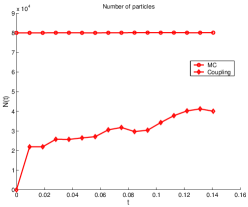
Figure 1: Two relaxation frequencies test: number of particles in time for the Monte Carlo scheme and the DSMC-Fluid Coupling.

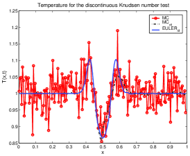
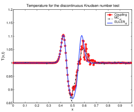
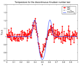
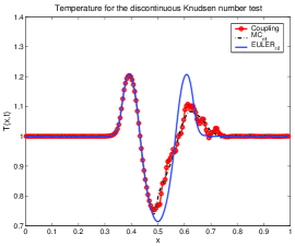
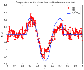
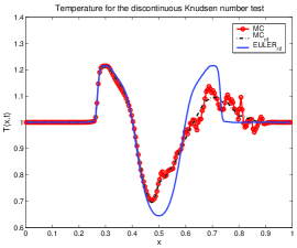
Figure 2: Two relaxation frequencies test: Solution at $t=0.05$ (top), $t=0.10$ (middle) and $t=0.15$ (bottom) for the temperature. MC method (left), Coupling DSMC-Fluid method (right). Knudsen number $\varepsilon=10^{-4}$ in the left half of the domain and Knudsen number $\varepsilon=10^{-2}$ in the right half of the domain. Reference solution (dotted line), Euler solution (continuous line), DSMC-Fluid or DSMC (circles plus continuous line).

7.3 Unsteady shock tests

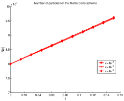
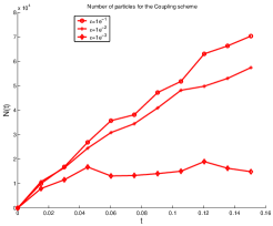
Figure 3: Unsteady Shock Test: Number of particle in time for the Monte Carlo scheme (left) and the DSMC-Fluid Coupling (right) for different values of the Knudsen Number (from $\varepsilon=10^{-1}$ to $\varepsilon=10^{-3}$).

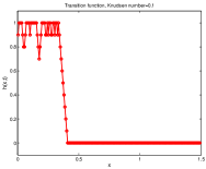
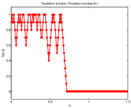
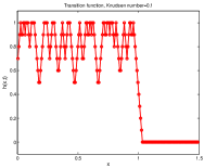
Figure 4: Unsteady Shock Test: Transition function at $t=0.05$ (left), $t=0.10$ (right) and $t=0.15$ (bottom). Knudsen number $\varepsilon=10^{-1}$.

We consider an unsteady shock that propagates from left to right in the computational domain $x=0$, $x=1.5$ discretized with $200$ cells in space. The number of particles is such that $400$ particles correspond to $\varrho=1$. The shock is produced pushing a gas against a wall which is located on the left boundary. In our test the particles are specularly reflected and the wall adopts the temperature of the gas instantaneously. The gas is supposed in thermodynamic equilibrium at the beginning of the simulation. The computation is stopped at the final time $t=0.15$. The transition function $h$ is initialized as $h=0$ (fluid region) everywhere.

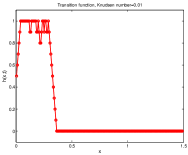
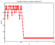
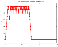
Figure 5: Unsteady Shock Test: Transition function at $t=0.05$ (left), $t=0.10$ (right) and $t=0.15$ (bottom). Knudsen number $\varepsilon=10^{-2}$.

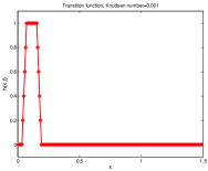
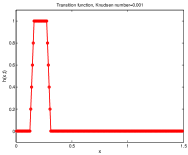
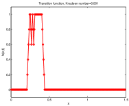
Figure 6: Unsteady Shock Test: Transition function at $t=0.05$ (left), $t=0.10$ (right) and $t=0.15$ (bottom). Knudsen number $\varepsilon=10^{-3}$.

We repeat the test with the same initial data $\varrho=1$, $u=-2$ and $T=4$, but changing the collision frequency. The relaxation parameter is $\varepsilon=10^{-1}$ in the first case, $\varepsilon=10^{-2}$ in the second case and $\varepsilon=10^{-3}$ in the last case. The thickness of the transition regions is fixed for every test depending on the frequency of collisions: ten cells for $\varepsilon=10^{-1}$ and $\varepsilon=10^{-2}$ while five cells for $\varepsilon=10^{-3}$.

In figure 3 we have reported the number of particles in time for the DSMC method (left) and the coupling method (right) for the different values of the frequency. As expected this number is independent from the choice of $\varepsilon$ for the DSMC method while in the case of the coupling the quantity of particles used varies strongly. This number is a measure of the computational cost of the method, the coupling procedure being computationally not expensive as well as the moment guided method and the solution of the fluid equations. In figure 4 the transition function is depicted for three different times in the case of $\varepsilon=10^{-1}$. The same function is depicted in figure 5 for $\varepsilon=10^{-2}$ and in figure 6 for $\varepsilon=10^{-3}$. These figures show the dynamics of the kinetic and fluid regions in time and the capability of the method to follow the shock which moves in the domain. We remark also that the thickness of the kinetic region decreases when the collision frequency increases as expected.

In figure 7 we have reported the density on the left for the DSMC method and the on the right for the DSMC/Fluid coupling. In this figure $\varepsilon=10^{-1}$. From top to bottom, time increases from $t=0.05$ (top) to $t=0.15$ (bottom) with $t=0.1$ in the middle. In each of the plots we reported the solution computed with our coupling method or with the DSMC method. The solution of the compressible Euler equation and a reference solution are also reported. The reference solution has been computed with a DMSC method where the number of particles is taken very high to reduce the statistical fluctuations

In figure 8 the density is reported for $\varepsilon=10^{-2}$ again for DSMC on the left and DSMC/Fluid coupling on the right. Finally we report the same results in the case of $\varepsilon=10^{-3}$ in figure 9.

During the simulation on the left boundary, the transition function $h$ increases from zero to one, which means that the solution is computed with the DSMC scheme, while in the rest of the domain the solution is still computed with the fluid scheme ($h=0$). When the shock starts to move towards the right the kinetic region increases. We observe that, in the case of $\varepsilon=10^{-3}$, when the shock is far from the left boundary the gas returns to thermodynamical equilibrium and thus automatically $h$ becomes equal to $0$. This is an interesting results because it shows that the method is able to recover an equilibrium regime after a time span in which it was in non equilibrium. While this results is not surprising when a deterministic scheme is used to solve the kinetic model, this is not obvious in the case of a DSMC solution of the kinetic equation because of the fluctuations which prevent the good evaluation of the macroscopic quantities needed to calculate the breakdown of the fluid model.

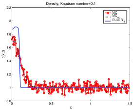
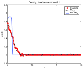
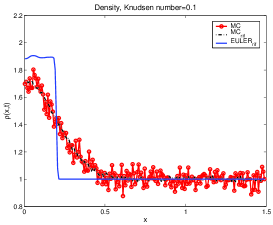
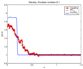
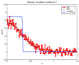
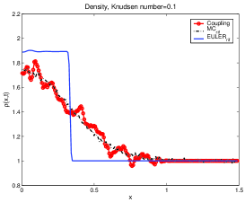
Figure 7: Unsteady Shock Test: Solution at $t=0.05$ (top), $t=0.10$ (middle) and $t=0.15$ (bottom) for the density. MC method (left), Coupling DSMC-Fluid method (right). Knudsen number $\varepsilon=10^{-1}$. Reference solution (dotted line), Euler solution (continuous line), DSMC-Fluid or DSMC (circles plus continuous line).

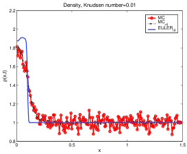
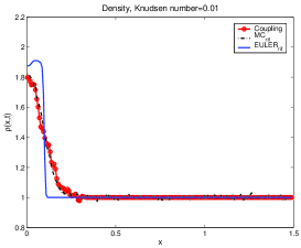
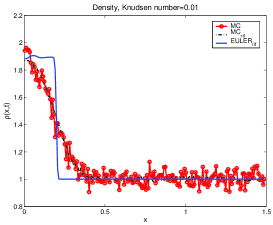
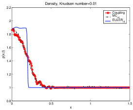
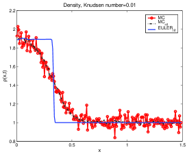
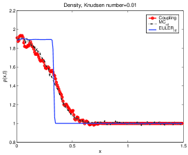
Figure 8: Unsteady Shock Test: Solution at $t=0.05$ (top), $t=0.10$ (middle) and $t=0.15$ (bottom) for the density. MC method (left), Coupling DSMC-Fluid method (right). Knudsen number $\varepsilon=10^{-2}$. Reference solution (dotted line), Euler solution (continuous line), DSMC-Fluid or DSMC (circles plus continuous line).

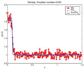
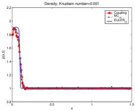
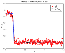
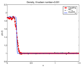
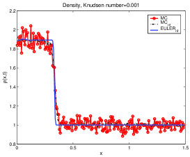
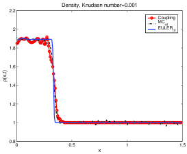
Figure 9: Unsteady Shock Test: Solution at $t=0.05$ (top), $t=0.10$ (middle) and $t=0.15$ (bottom) for the density. MC method (left), Coupling DSMC-Fluid method (right). Knudsen number $\varepsilon=10^{-3}$. Reference solution (dotted line), Euler solution (continuous line), DSMC-Fluid or DSMC (circles plus continuous line).

7.4 Sod tests

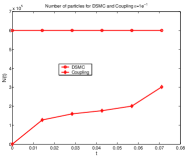
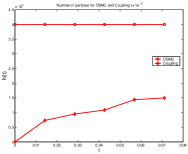
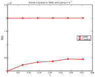
Figure 10: Sod Test: Number of particle in time for the Monte Carlo scheme and the DSMC-Fluid Coupling. Knudsen Number $\varepsilon=10^{-1}$ (left), $\varepsilon=10^{-2}$ (middle), $\varepsilon=10^{-3}$ (right).

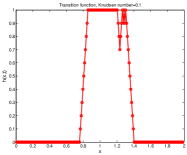
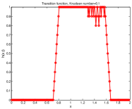
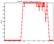
Figure 11: Sod Test: Transition function at $t=0.3$ (left), $t=0.6$ (middle) and $t=0.8$ (right). Knudsen number $\varepsilon=10^{-1}$.

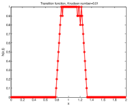
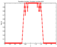
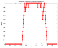
Figure 12: Sod Test: Transition function at $t=0.3$ (left), $t=0.6$ (middle) and $t=0.8$ (right). Knudsen number $\varepsilon=10^{-2}$.

In this final series of tests, we consider the classical Sod initial data in a domain which ranges from $0$ to $2$. The numerical parameters are the following: $200$ mesh points in space while the number of particles is chosen different for different values of the collision frequency. In this test case, we choose a larger number particles, in comparison to the previous tests, to show that the method is able to reproduce the correct profiles of the solutions. The number of particles needed to keep the statistical noise sufficiently low is a function of the perturbation $g_{K}$. In fact, smaller is the perturbation, smaller is the statistical error in the moment guided method. Observe anyway that, the classical DSMC with the same number of particles still exhibits some important fluctuations. The computation is stopped at the final time $t=0.8$. Finally the simulations are initialized in the thermodynamic equilibrium case, i.e. $h=0$ everywhere.

We take the following initial conditions: mass density $\varrho_{L}=1$, mean velocity $u_{L}=0$ and temperature $T_{L}=5$ if $0\leq x\leq 1$, while $\varrho_{R}=0.125$, $u_{R}=0$, $T_{R}=4$ if $1\leq x\leq 2$. We repeat the same test changing the collision frequency. They are respectively such that $\varepsilon=10^{-1}$ in the first case, $\varepsilon=10^{-2}$ in the second case and $\varepsilon=10^{-3}$ in the last case. The thickness of the transition regions is fixed for every test depending on the Knudsen: ten cells for large Knudsen ($10^{-1}$ and $10^{-2}$) and five cells for small Knudsen ($10^{-3}$).

In figure 10 we have reported the number of particles in time for the DSMC method and the coupling method for different values of the frequency $\varepsilon^{-1}$ ($\varepsilon=10^{-1}$ left, $\varepsilon=10^{-2}$ middle, $\varepsilon=10^{-3}$ right). The initial number of particles (i.e. the number of particles used to represent the entire solution) is both for the DSMC and the coupling $6\ 10^{5}$ for $\varepsilon=10^{-1}$, $4\ 10^{5}$ for $\varepsilon=10^{-2}$ and $2\ 10^{5}$ for $\varepsilon=10^{-3}$. These numbers are a measure of the computational cost of the method as explained in the previous paragraph. In figure 11 the transition function is depicted for three different times in the case of $\varepsilon=10^{-1}$. The same function is depicted in figure 12 for $\varepsilon=10^{-2}$ and in figure 13 for $\varepsilon=10^{-3}$. These figures shows the dynamics of the kinetic and fluid regions in time and the capability of the method to follow not only the shock but also regions in which the departure from the equilibrium is smaller and which moreover moves in the domain. We remark also that the thickness of the kinetic region decreases when the collision frequency increases as expected. We observe that the transition function oscillates in time. This is due to the statistical fluctuations of the Monte Carlo scheme. If a more precise evaluation of the zones far from equilibrium is needed, it is sufficient to increase the number of particles. However, we point out that even with an oscillatory behavior of the transition function the profiles of the solution are very well captured.

In figure 14 we have reported the velocity profile on the left for the DSMC method and the on the right for the DSMC/Fluid coupling. In this figure the collision frequency is taken equal to $\varepsilon=10^{-1}$. From top to bottom, time increases from $t=0.3$ (top) to $t=0.8$ (bottom) with $t=0.6$ in the middle. In each of the plots regarding the macroscopic variables we reported the solution computed with our coupling method or with the DSMC method, a reference solution computed with a DMSC method where the number of particles is taken very high to reduce the statistical fluctuations and the solution of the compressible Euler equations.

In figures 15 the velocity profile is reported for $\varepsilon=10^{-2}$ again for DSMC on the left and DSMC/Fluid coupling on the right. Finally we report the results in the case of $\varepsilon=10^{-3}$ in figures 16 using the same visualisation criterion of the previous cases.

In spite of the complexity of the solution (in this case we have more than one zone which is potentially in non equilibrium), the algorithm shows a very good behavior. In particular, in the last case, the non equilibrium region is very tiny. Therefore, we largely reduce the computational cost and we do not lose accuracy in the description of the problem.

8 Conclusion

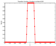
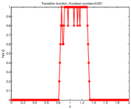
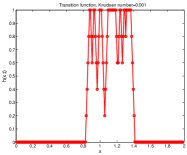
Figure 13: Sod Test: Transition function at $t=0.3$ (left), $t=0.6$ (middle) and $t=0.8$ (right). Knudsen number $\varepsilon=10^{-3}$.

In this paper, we have presented a novel numerical algorithm to couple a DSMC method for the solution of the Boltzmann equation and a finite volume like method for the compressible Euler equations. The method is based on the introduction of a buffer zone which realizes a smooth transition between the kinetic and fluid regions which was first introduced by Degond, Jin and Mieussens in [14]. Succesively, this method was extended to the case of moving interfaces in [16] and in [17].

Here, we have extended the idea of buffer zones and dynamic coupling to the case in which Monte Carlo methods are used to solve the kinetic equation. This extension permits to treat more detailed physical models than in the past. In particular it permits to resolve the Boltzmann collision integral instead of simplified relaxation models. In order to better adapt the coupling methodology to the case of DSMC methods, the coupling terms have been rearranged in a different way respect to the past which make the coupling more suitable for Monte Carlo approximations. Moreover, to reduce the fluctuations caused by Monte Carlo methods which produce spurious oscillations in the fluid regions, we used a new technique which permits to reduce the variance of particle methods [11]. This technique, called moment guided, is based on matching the moments of the kinetic solution with the moments of a suitable set of macroscopic equations which contains reduced statistical error at each time step of the computation. In addition, the use of this method permits a more precise estimation of the breakdowns of the fluid model. This is true even when few particles, in comparison with the typical number of particle employed in unsteady computations, are used.

The last part of the present work is centered on the analysis of several numerical tests. The results clearly demonstrate the capability of the method to couple Monte Carlo method with finite volume methods even for unsteady problems and with a relatively small number of particles. The resulting method is able to automatically create, cancel and move as many kinetic, fluid or buffer regions as necessary. It is also able to capture the correct solutions, to reduce the computational cost with respect to full DSMC simulations and to avoid the propagation of fluctuations in the fluid regions.

We finally observe that the computational speed-up will significantly increase for two or three dimensional simulations, which we intend to carry out in the future.

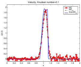
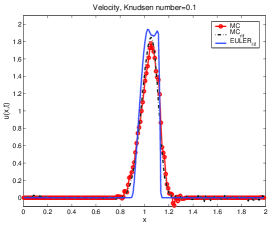
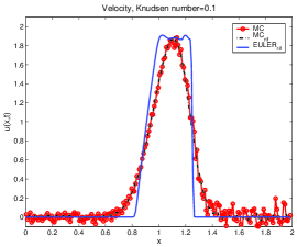
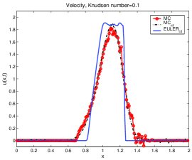
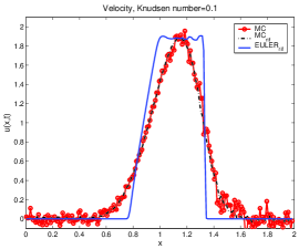
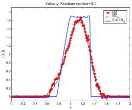
Figure 14: Sod Test: Solution at $t=0.3$ (top), $t=0.6$ (middle) and $t=0.8$ (bottom) for the velocity. MC method (left), Coupling DSMC-Fluid method (right). Knudsen number $\varepsilon=10^{-1}$. Reference solution (dotted line), Euler solution (continuous line), DSMC-Fluid or DSMC (circles plus continuous line).

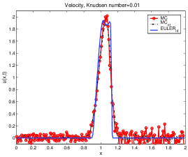
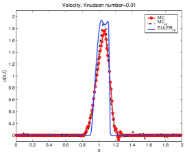
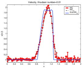
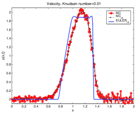
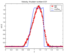
Figure 15: Sod Test: Solution at $t=0.3$ (top), $t=0.6$ (middle) and $t=0.8$ (bottom) for the velocity. MC method (left), Coupling DSMC-Fluid method (right). Knudsen number $\varepsilon=10^{-2}$. Reference solution (dotted line), Euler solution (continuous line), DSMC-Fluid or DSMC (circles plus continuous line).

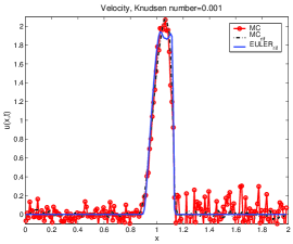
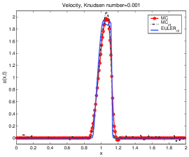
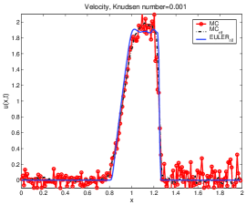
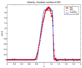
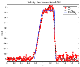
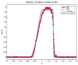
Figure 16: Sod Test: Solution at $t=0.3$ (top), $t=0.6$ (middle) and $t=0.8$ (bottom) for the velocity. MC method (left), Coupling DSMC-Fluid method (right). Knudsen number $\varepsilon=10^{-3}$. Reference solution (dotted line), Euler solution (continuous line), DSMC-Fluid or DSMC (circles plus continuous line).

References

- [1] O. Aktas, and N.R. Aluru, A combined continuum/DSMC technique for multiscale analysis of microfluidic filters. J. Comp. Phys., vol.178, (2002) pp. 342–72.
- [2] H. Babovsky, On a simulation scheme for the Boltzmann equation, Math. Methods Appl. Sci., 8 (1986), pp. 223–233.
- [3] G.A.Bird, Molecular gas dynamics and direct simulation of gas flows, Clarendon Press, Oxford (1994).
- [4] J. F. Bourgat, P. LeTallec, B. Perthame, and Y. Qiu, Coupling Boltzmann and Euler equations without overlapping, in Domain Decomposition Methods in Science and Engineering, Contemp. Math. 157, AMS, Providence, RI, (1994), pp. 377–398.
- [5] J. F. Bourgat, P. LeTallec, M.D. Tidriri, Coupling Boltzmann and Navier-Stokes equations by friction. J. Comput. Phys. 127, vol. 2 (1996), pag. 227–245.
- [6] J. Burt, I. Boyd, A low diffusion particle method for simulating compressible inviscid flows, J. Comput. Phys., Volume 227, Issue 9, 20 April 2008, pp. 4653-4670
- [7] J. Burt, I. Boyd, A hybrid particle approach for continuum and rarefied flow simulation, J. Comput. Phys., Vol. 228, (2009), pp. 460-475.
- [8] R. E. Caflisch, Monte Carlo and Quasi-Monte Carlo Methods, Acta Numerica (1998) pp. 1–49.
- [9] C. Cercignani, The Boltzmann Equation and Its Applications, Springer-Verlag, New York, (1988).
- [10] N.Crouseilles, P.Degond, M.Lemou, A hybrid kinetic-fluid model for solving the gas-dynamics Boltzmann BGK equation, J. Comput. Phys., vol. 199 (2004), pp. 776-808.
- [11] P. Degond, G. Dimarco, L. Pareschi, The Moment Guided Monte Carlo Method, To appear in International Journal for Numerical Methods in Fluids.
- [12] P. Degond, G. Dimarco, L. Pareschi, G. Russo, Moment Guided Monte Carlo Schemes for the Boltzmann equation, Work in Progress 2010.
- [13] P. Degond, S. Jin, A Smooth Transition Between Kinetic and Diffusion Equations, SIAM J. Numer. Anal., vol. 42 6 (2004), pp. 2671–2687.
- [14] P. Degond, S. Jin, L. Mieussens, A Smooth Transition Between Kinetic and Hydrodynamic Equations , J. Comput. Phys., vol. 209 (2005), pp. 665-694.
- [15] P.Degond, J.-G. Liu, L. Mieussens, Macroscopic fluid models with localized kinetic upscaling effects, SIAM MMS, vol. 5 (2006), pp. 940-979.
- [16] P. Degond, G. Dimarco, L. Mieussens., A Moving Interface Method for Dynamic Kinetic-fluid Coupling. J. Comp. Phys., Vol. 227, pp. 1176-1208, (2007).
- [17] P. Degond, G. Dimarco, L. Mieussens., A Multiscale Kinetic-Fluid Solver With Dynamic Localization Of Kinetic Effects. J. Comp. Phys., Vol. 229, pp. 4907-4933, (2010).
- [18] G. Dimarco and L. Pareschi, Domain decomposition techniques and hybrid multiscale methods for kinetic equations, Proceedings of the 11th International Conference on Hyperbolic problems: Theory, Numerics, Applications, pp. 457-464.
- [19] D.B. Hash and H.A. Hassan, Assessment of schemes for coupling Monte Carlo and Navier-Stokes solution methods, J. Thermophys. Heat Transf., 10, (1996), pp. 242–249.
- [20] A. Klar and C. Schmeiser, Numerical passage from radiative heat transfer to nonlinear diffusion models, Math. Models Methods Appl. Sci., Vol. 11, pp.749- 767, 2001.
- [21] V.I. Kolobov, R.R. Arslanbekov,V.V. Aristov, A.A. Frolova, S.A. Zabelok, Unified Solver for Rarefied and Continuum Flows with Adaptive Mesh and Algorithm Refinement, J. Comput. Phys., Vol. 223 No. 2, pp. 589–608 (2007).
- [22] D. Levermore, W.J.Morokoff, B.T. Nadiga, Moment realizability and the validity of the Navier Stokes equations for rarefied gas dynamics, Physics of Fluids, Vol. 10, No. 12, (1998).
- [23] P. LeTallec and F. Mallinger, Coupling Boltzmann and Navier-Stokes by half fluxes J. Comput. Phys., vol .136 (1997), pp. 51–67.
- [24] K. Nanbu, Direct simulation scheme derived from the Boltzmann equation, J. Phys. Soc. Japan, vol. 49 (1980), pp. 2042–2049.
- [25] R. Roveda, D.B. Goldstein, and P.L. Varghese, Hybrid Euler/Particle Approach for Continuum/ Rarefied Flows, AIAA J. Spacecraft Rockets 35, (1998), pp. 258–265.
- [26] R. Roveda, D.B. Goldstein, and P.L. Varghese, Hybrid Euler/Direct Simulation Monte Carlo Calculation of Unsteady Slit Flow, AIAA J. Spacecraft Rockets, vol. 37 (2000), pp. 753-760.
- [27] T. Schulze, P. Smereka and W. E, Coupling kinetic Monte-Carlo and continuum models with application to epitaxial growth, J. Comput. Phys., vol. 189 (2003), pp. 197–211.
- [28] S. Tiwari, and A. Klar, An adaptive domain decomposition procedure for Boltzmann and Euler equations. J. Comp. Appl. Math., vol.90, (1998) pp. 223–37.
- [29] S. Tiwari, Coupling of the Boltzmann and Euler equations with automatic domain decomposition, J. Comput. Phys., vol. 144, 1998, 710–726.
- [30] S. Tiwari, A. Klar, S. Hardt, A Particle Particle Hybrid Method for Kinetic and Continuum Equations, J. Comput. Phys., Vol. 228, (2009) pp. 7109-7124.
- [31] W.-L. Wang and I. D. Boyd, Predicting Continuum breakdown in Hypersonic Viscous Flows, Phys. Fluids, Vol. 15, 2003, pp 91-100.
- [32] Q. Sun, I. D. Boyd, G. V. Candler, A hybrid continuum/particle approach for modeling subsonic, rarefied gas flows J. Comput. Phys., vol. 194, (2004) pp. 256-277.
- [33] T.E. Schwartzentruber, L.C. Scalabrin, I.D. Boyd, A modular particle continuum numerical method for hypersonic non-equilibrium gas flows J. Comput. Phys., Vol. 225 (2007), pp. 1159-1174.
- [34] D.C. Wadsworth, D.A. Erwin Two dimensional hybrid continuum/particle simulation approach for rarefied hypersonic flows. AIAA Paper 92-2975, 1992.
- [35] H.S. Wijesinghe, N.G. Hadjiconstantinou, Discussion of Hybrid Atomistic-Continuum Methods for Multiscale Hydrodynamics. Int. J. Multi. Comp. Eng., Vol.2 pp. 189 202(2004).
- [36] H.S. Wijesinghe, R.D. Hornung, A. L. Garcia, N. G. Hadjiconstantinou, Three dimensional hybrid continuum-atomistic simulations for multiscale hydrodynamics. J. Fluids Eng., Vol. 126, pp. 768-777, 2004.