On the spectral vanishing viscosity method for periodic fractional conservation laws

Abstract.

We introduce and analyze a spectral vanishing viscosity approximation of periodic fractional conservation laws. The fractional part of these equations can be a fractional Laplacian or other non-local operators that are generators of pure jump Lévy processes. To accommodate for shock solutions, we first extend to the periodic setting the Kružkov-Alibaud entropy formulation and prove well-posedness. Then we introduce the numerical method, which is a non-linear Fourier Galerkin method with an additional spectral viscosity term. This type of approximation was first introduced by Tadmor for pure conservation laws. We prove that this non-monotone method converges to the entropy solution of the problem, that it retains the spectral accuracy of the Fourier method, and that it diagonalizes the fractional term reducing dramatically the computational cost induced by this term. We also derive a robust $L^{1}$-error estimate, and provide numerical experiments for the fractional Burgers’ equation.

1. Introduction

In this paper we are concerned with a spectral vanishing viscosity (henceforth SVV) approximation for periodic solutions of non-local or fractional conservation laws of the form

$$\left\{\begin{array}[]{ll}\partial_{t}u+\partial_{x}\cdot f(u)=-(-\Delta)^{\lambda/2}u,&(x,t)\in D_{T}\\ u(x,0)=u_{0}(x),&x\in\Lambda,\end{array}\right.$$

for $\lambda\in(0,2)$, or more generally, for

(1.1) $$\left\{\begin{array}[]{ll}\partial_{t}u+\partial_{x}\cdot f(u)=\mathcal{L}^{\mu}[u],&(x,t)\in D_{T}\\ u(x,0)=u_{0}(x),&x\in\Lambda,\end{array}\right.$$

where $D_{T}=\Lambda\times(0,T)$ and $\Lambda=(0,2\pi)^{d}$, and $\mathcal{L}^{\mu}[\cdot]$ is a non-local (Lévy type) operator defined as

(1.2) $$\mathcal{L}^{\mu}[\phi(\cdot)](x)=\int_{|z|>0}\phi(x+z)-\phi(x)-z\cdot\partial_{x}\phi(x)\,\mathbf{1}_{|z|<1}\ \mathrm{d}\mu(z),$$

where $\mathbf{1}(\cdot)$ is the indicator function. Throughout the paper we assume that

(A.1) $$f=(f_{1},\ldots,f_{d})\text{ with }f_{j}\in C^{s}(\mathbb{R})\text{ for all }j=1,\ldots,d\text{ ($s$ to be defined)};$$

(A.2) $$\text{$\mu\geq 0$ is a Radon measure such that $\int_{|z|>0}|z|^{2}\wedge 1\ \mathrm{d}\mu(z)<\infty$};$$

(A.3) $$u_{0}\in L^{\infty}(\Lambda)\cap BV(\Lambda),\text{ $u_{0}$ is $\Lambda$-periodic}.$$

Here and in the rest of the paper, $a\wedge b=\min(a,b)$,

$$\begin{split}\partial_{t}=\frac{\partial}{\partial t},\quad\partial_{j}=\frac{\partial}{\partial x_{j}}\quad\text{and}\quad\partial_{x}=(\partial_{1},\partial_{2},\ldots,\partial_{d}).\end{split}$$

Integro-PDEs like (1.1) typically model anomalous convection-diffusion phenomena. When $\mu=\pi_{\lambda}$ is defined by

(1.3) $$\begin{split}d\pi_{\lambda}(z)=\frac{c_{\lambda}}{|z|^{d+\lambda}}dz,\qquad c_{\lambda}>0\text{ and }\lambda\in(0,2),\end{split}$$

then $\mathcal{L}=-(-\Delta)^{\lambda/2}$ and the equation finds applications in e.g. over-driven detonation in gases [14] and anomalous diffusion in semiconductor growth [38]. Applications in dislocation dynamics, hydrodynamics and molecular biology can also be found, see e.g. the references in [1, 18]. Many more applications can be found if asymmetric measures $\mu$ are allowed. For example, we cover the (linear) option pricing equations for all Lévy models used in mathematical finance [15, 34], if

(1.4) $$\begin{split}d\mu(z)=g(z)\,d\pi_{\lambda}(z),\end{split}$$

for some possibly asymmetric locally Lipschitz continuous function $g(\cdot)$. An example is the one-dimensional ($d=1$) CGMY model where

$$g(z)=\left\{\begin{split}&Ce^{-G|z|}&\text{for $z>0$,}\\ &Ce^{-M|z|}&\text{for $z<0$,}\end{split}\right.$$

for positive constants $C,G,M$ (and $Y=\lambda$). In general the non-local operator $\mathcal{L}$ is the generator of a pure jump Lévy process, and conversely, any Lévy process will have generator like $\mathcal{L}$ when (A.2) is satisfied. We refer to the books [3, 15, 32] for more information about Lévy processes and their many applications. The most general Lévy measures for which the results of this paper applies, are Lévy measures $\mu$ that can be decomposed as

(1.5) $$\begin{split}\mu=\mu_{s}+\mu_{n},\end{split}$$

where

(1.6) $$\begin{split}\mu_{s},\mu_{n}\geq 0,\quad\mu_{s}\text{ is symmetric$\quad$and}\quad\int_{|z|>0}|z|\wedge 1\ \mathrm{d}\mu_{n}(z)<\infty.\end{split}$$

See Section 8 for statements of results and remarks. This class possibly includes all Lévy measures, but we have so far not found a proof of this. At least it includes all the Lévy measures found in finance, see Remark 8.3, and also many singular measures like e.g. delta-measures.

It is important to note that non-linear equations like (1.1) do not admit classical solutions in general, and that shock discontinuities can develop even from regular initial conditions. This is well known for pure conservations laws (where $\mathcal{L}=0$), see e.g. [23]. For fractional conservation laws where $\mathcal{L}=-(-\Delta)^{\lambda/2}$, it is shown in recent works that solutions are smooth for $\lambda\in[1,2)$ [8, 18, 26]. However, when $\lambda\in(0,1)$, the fractional diffusion is too weak to prevent shock discontinuities from forming, see [1, 10, 26]. In some cases however, these shocks are smoothed out over time [9]. When shocks form, weak solutions become non-unique and entropy conditions are needed to select the physically correct solution – the entropy solution. The well known Kružkov entropy solution theory for conservation laws was extended to fractional conservation laws in [1]. This extension relies on new ideas for the fractional term and is strongly influenced by the viscosity solution theory for fractional Hamilton-Jacobi-Bellman equations. Extensions of the Kružkov-Alibaud theory to general Lévy operators and even non-linear fractional terms can be found in [12, 25].

In this paper we deal with a SVV (spectral vanishing viscosity) approximation of $\Lambda$-periodic entropy solutions of (1.1). The method is a Fourier Galerkin method with an additional spectral viscosity term. Because of the formation of shocks in the solutions of (1.1), it is very difficult to devise a convergent and spectrally accurate numerical approximation of this equation. This has to do with the fact that Fourier spectral methods support spurious Gibbs oscillations, and thus fails to converge strongly toward discontinuous solutions. It is well known that such methods need to be augmented by some kind of vanishing viscosity in order to achieve convergence. But the standard vanishing viscosity method is not spectrally accurate. To overcome these problems, we use the SVV approximation developed by Tadmor in [35], cf. also [11, 30, 33, 36] and the books [4, 6]. To suppress spurious oscillations without sacrificing the overall spectral accuracy of the method, Tadmor adds a modified viscosity term, which in Fourier space only affects high frequencies. There are two parameters involved in this approach, the coefficient of the viscosity term $\varepsilon$ and the size $m$ of the viscosity free spectrum. Spectral accuracy and convergence toward the unique, possibly discontinuous, entropy solution, then follows by imposing appropriate conditions on $\epsilon$ and $m$. We also like to mention another important feature of the method. In all cases, it diagonalizes the fractional term and hence reduces dramatically the computational cost induced by this term. In our rather naive implementation for the fractional Burgers’ equation, the SVV method turned out to be orders of magnitude faster than a Discontinuous Galerkin approximation of the same equation where the fractional term gives full matrices.

When equation (1.1) is linear, $f(u)=u$, or when it is local $\mathcal{L}=0$, there is a vast literature on numerical methods and analysis, some methods and many references can be found e.g. in [4, 15, 23, 34]. In the general case however, there is not much work on numerical methods, we only know of the papers [13, 17, 21]. Difference methods are introduced in [17] for equation (1.1), and in [21] for an equation similar to (1.1) from radiation hydrodynamics. In [17], the first general convergence result for monotone schemes is obtained. Finally, in [13], a Discontinuous Galerkin approximation of (1.1) is analyzed and a Kuznetsov type of theory is established and used to derive error estimates. A periodic extension of this theory will be used to find error estimates in this paper.

Throughout the paper we will use the following additional notation. A subscript $p$ indicates $\Lambda$-periodicity in the space variables (i.e. in $L^{\infty}_{p}$ or $C^{\infty}_{p}$). Here $\Lambda$-periodic means $2\pi$-periodic in each coordinate direction. As a generic constant we use $C$. Note that the value of $C$ may change from line to line and expression to expression. We also need notation for high order derivatives and their norms. Let $\alpha=(\alpha_{1},\dots,\alpha_{d})$ be a multi index, then

$$\partial_{x}^{\alpha}=\partial_{1}^{\alpha_{1}}\partial_{2}^{\alpha_{1}}\cdots\partial_{d}^{\alpha_{d}},\quad\partial_{x}^{s}=\bigcup_{|\alpha|=s}\Big{\{}\partial_{x}^{\alpha}\Big{\}},\quad\text{and}\quad\|\partial^{s}_{x}\phi\|_{L^{p}}^{p}=\sum_{|\alpha|=s}\|\partial_{x}^{\alpha}\phi\|_{L^{p}}^{p}.$$

Remember that $\alpha_{j}\geq 0$, $|\alpha|=\alpha_{1}+\dots+\alpha_{d}$, and that $x^{\alpha}=x_{1}^{\alpha_{1}}\cdots x_{d}^{\alpha_{d}}$ for any $x\in\mathbb{R}^{d}$.

The rest of this paper is organized as follows. In Section 2 we introduce an entropy formulation for periodic solutions (1.1), and give a $L^{1}$-contraction and uniqueness result. In the same section we introduce the classical vanishing viscosity approximation of (1.1), and show convergence towards (1.1) with optimal $L^{1}$ error estimate. As a corollary we get existence for (1.1). The proofs rely on the Kružkov’s doubling of variables device [1, 27] and Kuznetsov type of arguments [13, 28], and are given in the Appendix. The SVV approximation of (1.1) is introduced in Section 3, and we show that it is spectrally accurate and that it diagonalizes the non-local operator. In sections 4–6, we assume that the measure $\mu$ is symmetric. In Section 4 we prove an energy estimate for the SVV method. Along with results from [11], this allows us to control the so-called ”truncation error”, the spectral projection error coming from the non-linear term. In Section 5 we prove a priori $L^{\infty}$, $BV$, and time regularity estimates for the SVV method, and obtain compactness. In Section 6 we prove that the SVV method converge to the classical vanishing viscosity method from Section 2. Combined with the results of that section, it follows that the SVV method converges to the entropy solution of (1.1). In the process, we also prove the optimal $L^{1}$-rate of convergence for our SVV approximation. We solve numerically, using our SVV method, the the fractional Burgers’ equation in Section 7. Finally, in Section 8 we extend the results in the previous sections to allow for asymmetric measures $\mu$.

2. Entropy formulation for periodic solutions

In this section we introduce an entropy formulation for $\Lambda$-periodic solutions of the initial value problem (1.1). To this end, we write the operator $\mathcal{L}^{\mu}[\cdot]$ as

$$\begin{split}\mathcal{L}^{\mu}[\phi]=\mathcal{L}_{r}^{\mu}[\phi]+\mathcal{L}^{\mu,r}[\phi]-\gamma_{\mu}^{r}\cdot\partial_{x}\phi,\end{split}$$

where

$$\begin{split}\mathcal{L}_{r}^{\mu}[\phi(\cdot)](x)&=\int_{|z|\leq r}\phi(x+z)-\phi(x)-z\cdot\partial_{x}\phi(x)\,\mathbf{1}_{|z|<1}\ \mathrm{d}\mu(z),\\ \mathcal{L}^{\mu,r}[\phi(\cdot)](x)&=\int_{|z|>r}\phi(x+z)-\phi(x)\ \mathrm{d}\mu(z),\\ \gamma_{\mu}^{r}&=\int_{r<|z|<1}z\ \mathrm{d}\mu(z).\end{split}$$

If $r>1$, we take $\gamma_{\mu}^{r}=0$. The adjoint of $\mathcal{L}^{\mu}[\cdot]$ takes the form

$$\begin{split}\mathcal{L}^{\ast,\mu}_{r}[\phi]=\mathcal{L}_{r}^{\ast,\mu}[\phi]+\mathcal{L}^{\ast,\mu,r}[\phi]+\gamma_{\mu}^{r}\cdot\partial_{x}\phi,\end{split}$$

where

$$\begin{split}\mathcal{L}_{r}^{\ast,\mu}[\phi(\cdot)](x)&=\int_{|z|\leq r}\phi(x-z)-\phi(x)+z\cdot\partial_{x}\phi(x)\,\mathbf{1}_{|z|<1}\ \mathrm{d}\mu(z),\\ \mathcal{L}^{\ast,\mu,r}[\phi(\cdot)](x)&=\int_{|z|>r}\phi(x-z)-\phi(x)\ \mathrm{d}\mu(z).\end{split}$$

We also let $\eta$, $\eta^{\prime}$, and $q$ denote the functions

$$\begin{split}\eta(u,k)=|u-k|,\quad\eta^{\prime}(u,k)=\mathrm{sgn}(u-k),\quad q_{j}(u,k)=\eta^{\prime}(u,k)\,(f_{j}(u)-f_{j}(k)).\end{split}$$

We now define the solution concept we will use in this paper.

Definition 2.1.

(Periodic entropy solutions) A function $u$ is a periodic entropy solution of the initial value problem (1.1) provided that

• $u\in C([0,T];L_{p}^{\infty}(\mathbb{R}^{d}))$;

• for all $k\in\mathbb{R}$, all $r>0$, and all nonnegative test functions $\varphi\in C_{p}^{\infty}(\mathbb{R}^{d}\times(0,T))$,

  (2.1) $$\begin{split}&\iint_{D_{T}}\eta(u,k)\,\partial_{t}\varphi+q(u,k)\cdot\partial_{x}\varphi\\ &\qquad+\eta(u,k)\,\mathcal{L}^{\ast,\mu}_{r}[\varphi]+\eta^{\prime}(u,k)\,\mathcal{L}^{\mu,r}[u]\,\varphi+\eta(u,k)\,\gamma_{\mu}^{r}\cdot\partial_{x}\varphi\ \mathrm{d}x\,\mathrm{d}t\geq 0;\end{split}$$

• $\mathrm{esslim}_{t\rightarrow 0}\|u(\cdot,t)-u_{0}(\cdot)\|_{L^{1}(\Lambda)}=0$.

Remark 2.1.

In the entropy inequality (2.1) it is easy to see that all the terms, except possibly the $\mathcal{L}^{\mu,r}$-term, are well defined and $\Lambda$-periodic in view of i). The problem with the $\mathcal{L}^{\mu,r}$-term is that we integrate a Lebesgue measurable function w.r.t. a Radon measure $\mu$. But the term is still well defined because the integrand of $\mathcal{L}^{\mu,r}[u]$ is measurable w.r.t. the product measure $\mathrm{d}\mu(z)\mathrm{d}x\mathrm{d}t$. This is true because the integrand is the $\mathrm{d}\mu(z)\mathrm{d}x\mathrm{d}t$-a.e. limit of continuous functions, a fact which readily follows from the fact that $u$ is the $\mathrm{d}x\mathrm{d}t$-a.e. limit of smooth functions. By i), (A.3), and Fubini, we then find that $\mathcal{L}^{\mu,r}[u]\in C([0,T];L^{\infty}_{p}(\mathbb{R}^{d}))$.

We now state the following central result:

Theorem 2.2.

($L^{1}$-contraction) Let $u$ and $v$ be two entropy solutions of the initial value problem (1.1) with initial data $u_{0}$ and $v_{0}$. Then, for a.e. $t\in(0,T)$,

(2.2) $$\|u(\cdot,t)-v(\cdot,t)\|_{L^{1}(\Lambda)}\leq\|u_{0}-v_{0}\|_{L^{1}(\Lambda)}.$$

The proof will be given in Appendix A. Uniqueness for periodic entropy solutions of (1.1) immediately follows by setting $u_{0}=v_{0}$.

Corollary 2.3.

(Uniqueness) There is at most one entropy solution of (1.1).

We now consider the vanishing viscosity approximation of (1.1),

(2.3) $$\left\{\begin{array}[]{ll}\partial_{t}u_{\epsilon}+\partial_{x}\cdot f(u_{\epsilon})=\mathcal{L}^{\mu}[u_{\epsilon}]+\epsilon\,\Delta u_{\epsilon}&(x,t)\in D_{T},\\ u_{\epsilon}(x,0)=u_{0}(x)&x\in\Lambda.\end{array}\right.$$

In this paper we always assume that this problem admits a unique classical solution $u_{\epsilon}$. This is of course true, but a proof lays outside the scope of this paper. Remark 2.6 below provides some ideas on how to prove this result. We now give an estimate on the rate of convergence of $u_{\varepsilon}$ toward the entropy solution $u$ of (1.1).

Theorem 2.4 (Convergence rate I).

Let $u$ be the periodic entropy solution of (1.1), and $u_{\epsilon}$ be a smooth solution of (2.3). Then,

(2.4) $$\begin{split}\|u(\cdot,t)-u_{\epsilon}(\cdot,t)\|_{L^{1}(\Lambda)}\leq C\,\sqrt{\epsilon}.\end{split}$$

The proof is given in Appendix B. This result generalizes to periodic fractional conservation laws Kuznetsov’s well known result for scalar conservation laws [28]. As a by-product of the well-posedness of (2.3) and Theorem 2.4, we have the existence of entropy solutions of (1.1).

Corollary 2.5.

(Existence) There exists an entropy solution of (1.1).

Remark 2.6.

Uniqueness of solutions of (2.3) can be proved using an entropy formulation (see the start of Appendix B) and a standard adaptation of the proof of Theorem 2.2 incorporating ideas of Carrillo [7] to handle the Laplace term. Existence of an entropy solution can be proven e.g. by appropriately modifying our spectral approximation, compactness, and convergence analysis, see the following sections. The solution of (2.3) will also be smooth. To see this, note that the principal term in (2.3) is the $\epsilon\Delta$-term while the $\mathcal{L}^{\mu}$-term is of lower order, and hence regularity proofs for viscous conservation laws ((2.3) with $\mu\equiv 0$ and $\varepsilon>0$) should still work after some modifications. We refer to e.g. [31] for regularity of viscous conservation laws, and note that the modifications typically consist of using interpolation inequalities for the $\mathcal{L}^{\mu}$-term, see e.g. Lemma 2.2.1 in [22].

3. The spectral vanishing viscosity method

We introduce a Fourier spectral method for the $d$-periodic initial value problem (1.1). The approximate solutions will be $N$-trigonometric polynomials,

$$\begin{split}u_{N}(x,t)=\sum_{|\xi|\leq N}\hat{u}_{\xi}(t)\,e^{i\xi\cdot x},\end{split}$$

which solve the semi-discrete spectral vanishing viscosity (SVV) approximation

(3.1) $$\begin{split}\partial_{t}u_{N}+\partial_{x}\cdot P_{N}f(u_{N})=\mathcal{L}^{\mu}[u_{N}]+\epsilon_{N}\sum_{j,k=1}^{d}\partial_{jk}^{2}Q_{N}^{j,k}\ast u_{N}\end{split}$$

with

(3.2) $$\begin{split}u_{N}(x,0)=P_{N}u_{0}(x),\end{split}$$

where the Fourier projection $P_{N}$ is defined as

$$P_{N}\phi(x)=\sum_{|\xi|\leq N}\hat{\phi}_{\xi}\,e^{i\xi\cdot x}\qquad\text{for}\qquad\hat{\phi}_{\xi}=\frac{1}{(2\pi)^{d}}\int_{\Lambda}\phi(x)\,e^{-i\xi\cdot x}\ \mathrm{d}x.$$

The (spectral) vanishing viscosity term has the following three ingredients:

• a vanishing viscosity amplitude $\epsilon_{N}\sim N^{-\theta}$ with $0<\theta<1$;

• a viscosity-free spectrum $m_{N}\sim N^{\frac{\theta}{2}}(\log N)^{-\frac{d}{2}}$;

• a family of viscosity kernels

  $$Q_{N}^{j,k}(x,t)=\sum_{p=m_{N}}^{N}\hat{Q}_{p}^{j,k}(t)\sum_{|\xi|=p}e^{i\xi\cdot x}$$

  satisfying

  • $\hat{Q}_{p}^{j,k}$ is monotonically $p$-increasing,

  • $\hat{Q}_{p}^{j,k}$ spherically symmetric, $\hat{Q}_{\xi}^{j,k}=\hat{Q}_{p}^{j,k}$ for all $|\xi|=p$,

  • $|\hat{Q}_{p}^{j,k}-\delta_{jk}|\leq C\,m_{N}^{2}\,p^{-2}$ for all $p\geq m_{N}$.

Such kernels can be conveniently implemented in Fourier space,

$$\begin{split}\sum_{j,k=1}^{d}\partial_{jk}^{2}Q_{N}^{j,k}\ast u_{N}=-\sum_{|\xi|=m_{N}}^{N}\left(\sum_{j,k=1}^{d}\hat{Q}_{\xi}^{j,k}(t)\,\xi_{j}\,\xi_{k}\right)\hat{u}_{\xi}(t)\,e^{i\xi\cdot x}.\end{split}$$

Combined with one’s favorite ODE solver (e.g. Euler, Runge-Kutta, etc.), (3.1) and (3.2) give a fully discrete numerical approximation method for (1.1).

With left-hand sides set to zero ($\mu\equiv 0$ and $\varepsilon_{N}=0$), (3.1) becomes the standard Fourier approximation of (1.1). It is well known that this approximation is spectrally accurate but, as opposed to the equation, it lacks entropy dissipation. The approximation supports spurious Gibbs oscillations which prevent strong convergence toward solutions containing shock discontinuities. If the $\mathcal{L}^{\mu}$-term is present in the equations, shock solutions are still possible in some situations [2], and the problem of the Gibbs oscillations remains. In order to suppress such oscillations without sacrificing the overall spectral accuracy of the method, we have followed Tadmor [35] and added a vanishing spectral viscosity term to the scheme, $\epsilon_{N}\sum_{j,k=1}^{d}\partial_{jk}^{2}Q_{N}^{j,k}\ast u_{N}$.

An important feature of Fourier method (3.1) is that it diagonalizes, and hence localizes, the non-local operator $\mathcal{L}^{\mu}[\cdot]$! This leads to dramatically reduced computational cost for this term. Indeed,

(3.3) $$\begin{split}\mathcal{L}^{\mu}[u_{N}]=\sum_{|\xi|\leq N}G^{\mu}(\xi)\,\hat{u}_{\xi}(t)\,e^{i\xi\cdot x},\end{split}$$

where

(3.4) $$\begin{split}G^{\mu}(\xi)=\int_{|z|>0}e^{i\xi\cdot z}-1-i\xi\cdot z\,\mathbf{1}_{|z|<1}\ \mathrm{d}\mu(z).\end{split}$$

Furthermore, when the measure $\mu$ is symmetric,

(3.5) $$\mu(-B)=\mu(B)\quad\text{for all Borel sets}\quad B\in\mathbb{R}^{d}\setminus\{0\},$$

the weights (3.4) are all real and non-positive. This follows since the imaginary part of the integrand is odd and the real part is even and non-positive ($e^{i\xi\cdot z}=\cos(\xi\cdot z)+i\,\sin(\xi\cdot z)$). Finally, we stress that the approximation of the non-local operator (1.2) is spectrally accurate since, by Taylor’s formula,

$$\begin{split}&\|\mathcal{L}^{\mu}[u_{N}(\cdot,t)]-\mathcal{L}^{\mu}[u(\cdot,t)]\|_{L^{2}(\Lambda)}\\ &\qquad\qquad\leq C\,\bigg{(}\sup_{j,k}\|\partial_{j}\partial_{k}(u_{N}-u)(\cdot,t)\|_{L^{2}(\Lambda)}+\|(u_{N}-u)(\cdot,t)\|_{L^{2}(\Lambda)}\bigg{)}.\end{split}$$

Now we define

$$\hat{R}_{\xi}^{j,k}(t)=\begin{cases}\delta_{jk}&|\xi|\leq m_{N},\\ \delta_{jk}-\hat{Q}_{\xi}^{j,k}(t)&|\xi|>m_{N},\end{cases}\qquad R_{N}^{j,k}(x,t)=\sum_{|\xi|\leq N}\hat{R}_{\xi}^{j,k}(t)\,e^{i\xi\cdot x},$$

and note that

(3.6) $$\begin{split}\Delta u_{N}(\cdot,t)=\sum_{j,k=1}^{d}\partial_{j}\partial_{k}Q_{N}^{j,k}(\cdot,t)\ast u_{N}(\cdot,t)+\sum_{j,k=1}^{d}\partial_{j}\partial_{k}R_{N}^{j,k}(\cdot,t)\ast u_{N}(\cdot,t).\end{split}$$

To conclude this section, we recall that by Lemma 3.1 and Corollary 3.2 of [11], the spectral vanishing viscosity term is an $L^{p}$-bounded perturbation of the standard vanishing viscosity $\epsilon_{N}\Delta u_{N}$:

Lemma 3.1.

For $0\leq r\leq s\leq 2$,

(3.7) $$\begin{split}\left\|\sum_{j,k=1}^{d}\partial_{j}^{r}\partial_{k}^{s-r}R_{N}^{j,k}(\cdot,t)\right\|_{L^{1}(\Lambda)}\leq C\,m_{N}^{s}\,(\log N)^{d}.\end{split}$$

Moreover, if $c_{N}\leq C\epsilon_{N}\,m_{N}^{2}\,(\log N)^{d}\leq\hat{C}$, then for all $p\geq 1$, $\varphi\in L^{p}(\Lambda)$,

(3.8) $$\begin{split}\epsilon_{N}\left\|\sum_{j,k=1}^{d}\partial_{j}\partial_{k}R_{N}^{j,k}(\cdot,t)\ast\varphi(\cdot)\right\|_{L^{p}(\Lambda)}\leq c_{N}\,\|\varphi\|_{L^{p}(\Lambda)}.\end{split}$$

4. Spectrally small truncation error for symmetric $\mu$

In this section we assume that the measure $\mu$ is symmetric, cf. (3.5). In the SVV approximation (3.1), the convection term $\partial_{x}\cdot f(u)$ is replaced by $\partial_{x}\cdot P_{N}f(u_{N})$ which leads to the (truncation) term error

$$\begin{split}\partial_{x}\cdot(I-P_{N})f(u_{N}).\end{split}$$

We will now show that this error is spectrally small due to the presence of the spectral vanishing viscosity term.

Let us start by noting that a straightforward estimate leads to

$$\begin{split}\|\partial_{x}^{\alpha}(I-P_{N})f(u_{N})\|_{L^{2}(\Lambda)}=\bigg{(}\sum_{j=1}^{d}\sum_{|\xi|>N}|\xi^{\alpha}|^{2}|\widehat{f_{j}(u_{N})}(\xi)|^{2}\bigg{)}^{\frac{1}{2}}\leq\frac{\|\partial_{x}^{\alpha+\beta}f(u_{N})\|_{L^{2}(\Lambda)}}{N^{|\beta|}}\end{split}$$

for all multi-indices $\alpha,\beta$. Note that there is no divergence in this estimate, so $\partial_{x}^{\alpha}f$ is a vector. By Theorem 7.1 in [11], there is a constant $\mathcal{K}_{s}$ such that

(4.1) $$\begin{split}\|\partial_{x}^{s}f(u_{N})\|_{L^{2}(\Lambda)}\leq\mathcal{K}_{s}\|\partial_{x}^{s}u_{N}\|_{L^{2}(\Lambda)}\quad\text{for}\quad\mathcal{K}_{s}\leq C\sum_{k=1}^{s}|f|_{C^{k}}\|u_{N}\|_{L^{\infty}(\Lambda)}^{k-1}\end{split}$$

and $s=1,2,\dots$, where $|f|_{C^{k}}=\|\partial_{x}^{k}f(\cdot)\|_{L^{\infty}(\Omega_{N})}$ and $\Omega_{N}=\{u:|u|\leq\|u_{N}\|_{L^{\infty}(\Lambda)}\}$. This inequality is a type of Gagliardo-Nirenberg-Moser estimate, and similar results can be found in page 22 in Taylor [37]. By these two inequalities we can conclude that, for all $0\leq r\leq s$,

(4.2) $$\begin{split}\|\partial_{x}^{r}(I-P_{N})f(u_{N})\|_{L^{2}(\Lambda)}\leq\frac{\mathcal{K}_{s}}{N^{s-r}}\,\|\partial_{x}^{s}u_{N}\|_{L^{2}(\Lambda)}.\end{split}$$

Inequality (4.2) states that the $r$-derivative of the truncation error decays as rapidly as the $s$-smoothness of $u_{N}$ permits. Of course the $s$-derivatives of an arbitrary $N$-trigonometric polynomial $u_{N}$ may grow as fast as $N^{s}$, in which case nothing is gained from (4.2). However, if $u_{N}$ is solves our VVS approximation (3.1), we can have the better bound $\epsilon_{N}^{-s}$ in $L^{2}$. This will be a consequence of the following energy estimate:

Theorem 4.1.

Consider the SVV approximation (3.1) with $\epsilon_{N}$ and $m_{N}$ such that

(A.7) $$\left\{\begin{split}&\epsilon_{N}>\frac{8\,d^{\frac{s}{2}}\mathcal{K}_{s+1}}{N},\\ &\epsilon_{N}\,m_{N}^{2}\,(\log N)^{d}\leq C.\end{split}\right.$$

Then there is a constant $\mathcal{B}_{s}$ (proportional to $\Pi_{k=1}^{s}\mathcal{K}_{s}$ for $s\geq 1$ and to $\|u_{N}\|_{L^{\infty}}$ for $s=0$) such that

(4.3) $$\begin{split}&\epsilon^{s}_{N}\|\partial_{x}^{s}u_{N}(\cdot,t)\|_{L^{2}(\Lambda)}+\epsilon^{s}_{N}\left(-\sum_{|\alpha|=s}\sum_{|\xi|\leq N}G^{\mu}(\xi)|\xi^{\alpha}|^{2}\int_{0}^{t}|\hat{u}_{\xi}(\tau)|^{2}\,\mathrm{d}\tau\right)^{\frac{1}{2}}\\ &\qquad\qquad\qquad+\epsilon_{N}^{s+\frac{1}{2}}\|\partial_{x}^{s+1}u_{N}\|_{L^{2}(D_{T})}\leq\mathcal{B}_{s}+3\epsilon_{N}^{s}\|\partial_{x}^{s}u_{N}(\cdot,0)\|_{L^{2}(\Lambda)}.\end{split}$$

Remember that in this section $\mu$ is symmetric and hence $G^{\mu}$ is real and non-positive. Now if

• $\quad|f|_{C^{s}}<\infty$ for sufficiently large $s$, cf. (4.7) below, and

• $\quad u_{0}$ is such that $\epsilon_{N}^{s}\,\|\partial_{x}^{s}u_{N}(\cdot,0)\|_{L^{2}(\Lambda)}\leq C$,

then Theorem 4.1 implies that

$$\begin{split}\|\partial_{x}^{s}u_{N}(\cdot,t)\|_{L^{2}(\Lambda)}\leq C\,\epsilon_{N}^{-s}\quad\text{and}\quad\|\partial_{x}^{s+1}u_{N}\|_{L^{2}(D_{T})}&\leq C\,\epsilon_{N}^{-(s+\frac{1}{2})}.\end{split}$$

Taking into account (4.2), we then find that

(4.4) $$\|\partial_{x}^{r}(I-P_{N})f(u_{N}(\cdot,t))\|_{L^{2}(\Lambda)} \leq C\,\mathcal{B}_{s}\,N^{-s_{r}},\quad s_{r}=s(1-\theta)-r,$$

(4.5) $$\|\partial_{x}^{r}(I-P_{N})f(u_{N})\|_{L^{2}(D_{T})} \leq C\,\mathcal{B}_{s}\,N^{-(s_{r}+\frac{\theta}{2})},\quad\forall\,s\geq 1.$$

We can now turn these inequalities into spectral decay estimates in the uniform norm using the Sobolev inequality (cf. Theorem 6, Chapter 5, in [20])

$$\begin{split}\|\partial_{x}^{r}\varphi\|_{L^{\infty}}\leq C\,\|\partial_{x}^{r+[\frac{d}{2}]+1}\varphi\|_{L^{2}}.\end{split}$$

For example, inequality (4.5) becomes

(4.6) $$\begin{split}\|\partial_{x}^{r}(I-P_{N})f(u_{N})\|_{L^{\infty}(D_{T})}&\leq C\,\mathcal{B}_{s}\,N^{-s_{r}+[\frac{d}{2}]+1-\frac{\theta}{2}}\leq C\,\mathcal{B}_{s}\,N^{-s_{r}+[\frac{d}{2}]+1}.\end{split}$$

Note that the polynomial decay rate in (4.6) can be made as large as the $C^{s}$-smoothness of $f(\cdot)$ permits. Taking $r=2$, we can find the following result.

Theorem 4.2.

If $f\in C^{s}$ with

(4.7) $$\begin{split}s\geq\frac{4+[\frac{d}{2}]}{1-\theta},\end{split}$$

then

(4.8) $$\begin{split}\|\partial_{x}(I-P_{N})f(u_{N})\|_{L^{\infty}(D_{T})}+\|\partial_{x}^{2}(I-P_{N})f(u_{N})\|_{L^{\infty}(D_{T})}\leq\frac{C\,\mathcal{B}_{s}}{N}.\end{split}$$

The smoothness requirement (4.7) will be sufficient for all the estimates derived throughout the paper.

Proof of Theorem 4.1.

For sake of brevity, we will write $\|\cdot\|$ instead of $\|\cdot\|_{L^{2}(\Lambda)}$. With (3.6) in mind, we rewrite the SVV approximation (3.1) in the two equivalent forms

(4.9) $$\begin{split}\partial_{t}u_{N}+\partial_{x}\cdot P_{N}f(u_{N})-\mathcal{L}^{\mu}[u_{N}]-\epsilon_{N}\Delta u_{N}=-\epsilon_{N}\sum_{j,k=1}^{d}\partial_{j}\partial_{k}R^{j,k}_{N}\ast u_{N},\end{split}$$

(4.10) $$\begin{split}&\partial_{t}u_{N}+\partial_{x}\cdot f(u_{N})-\mathcal{L}^{\mu}[u_{N}]-\epsilon_{N}\Delta u_{N}\\ &\qquad\qquad\qquad\qquad=-\epsilon_{N}\sum_{j,k=1}^{d}\partial_{j}\partial_{k}R^{j,k}_{N}\ast u_{N}+\partial_{x}\cdot(I-P_{N})f(u_{N}).\end{split}$$

Since $G^{\mu}(\xi)\leq 0$ ($\mu$ is symmetric) and $u_{N}(x)$ and $\mathcal{L}^{\mu}[u_{N}]$ are real,

$$\int_{\Lambda}\mathcal{L}^{\mu}[u_{N}]u_{N}\ \mathrm{d}x=\sum_{|\xi|\leq N}G^{\mu}(\xi)|\hat{u}_{\xi}(t)|^{2}\leq 0,$$

and hence spatial integration of (4.10) against $u_{N}$ yields

$$\begin{split}&\frac{1}{2}\frac{\mathrm{d}}{\mathrm{d}t}\|u_{N}\|^{2}-\sum_{|\xi|\leq N}G^{\mu}(\xi)|\hat{u}_{\xi}(t)|^{2}+\epsilon_{N}\|\partial_{x}u_{N}\|^{2}\\ &\leq\epsilon_{N}\|u_{N}\|\bigg{\|}\sum_{j,k=1}^{d}\partial_{j}\partial_{k}R_{N}^{j,k}\ast u_{N}\bigg{\|}+\sum_{j=1}^{d}\|\partial_{j}u_{N}\|\|(I-P_{N})f_{j}(u_{N})\|.\end{split}$$

Using (3.8) with $p=2$ for the first term on the right and (4.2) with $(r,s)=(0,1)$ for the second term, we find that

$$\begin{split}\frac{1}{2}\frac{\mathrm{d}}{\mathrm{d}t}\|u_{N}\|^{2}-\sum_{|\xi|\leq N}G^{\mu}(\xi)|\hat{u}_{\xi}(t)|^{2}+\left(\epsilon_{N}-\frac{\mathcal{K}_{1}}{N}\right)\|\partial_{x}u_{N}\|^{2}\leq c_{N}\|u_{N}\|^{2}\end{split}$$

with $c_{N}\leq C\epsilon_{N}\,m_{N}^{2}\,(\log N)^{d}\leq\hat{C}$. Hence (4.3) follows for $s=0$ since by (A.7),

$$\begin{split}\left(\epsilon_{N}-\frac{\mathcal{K}_{1}}{N}\right)>\frac{\epsilon_{N}}{2},\end{split}$$

and $c_{N}\|u_{N}\|^{2}\leq C\,\|u_{N}\|_{L^{\infty}(\Lambda)}^{2}=\mathcal{B}_{0}^{2}$.

The general case follows by induction on $s$. Spatial integration of (4.9) against $\partial_{x}^{2\alpha}u_{N}$ for some multi-index $\alpha$ yields

(4.11) $$\begin{split}&\frac{1}{2}\frac{\mathrm{d}}{\mathrm{d}t}\|\partial_{x}^{\alpha}u_{N}\|^{2}-\sum_{|\xi|\leq N}G^{\mu}(\xi)|\xi^{\alpha}|^{2}|\hat{u}_{\xi}(t)|^{2}+\epsilon_{N}\|\partial^{\alpha}_{x}\partial_{x}u_{N}\|^{2}\\ &\leq\epsilon_{N}\|\partial_{x}^{\alpha}u_{N}\|\bigg{\|}\sum_{j,k=1}^{d}\partial_{j}\partial_{k}R_{N}^{j,k}\ast\partial_{x}^{\alpha}u_{N}\bigg{\|}+\|\partial_{x}^{\alpha}\partial_{x}u_{N}\|\|\partial_{x}^{|\alpha|-1}\partial_{x}\cdot P_{N}f(u_{N})\|.\end{split}$$

After having used (3.8) and Young’s inequality to bound the first and second term on the right hand side, we find that

$$\begin{split}&\frac{1}{2}\frac{\mathrm{d}}{\mathrm{d}t}\|\partial_{x}^{\alpha}u_{N}\|^{2}-\sum_{|\xi|\leq N}G^{\mu}(\xi)|\xi^{\alpha}|^{2}|\hat{u}_{\xi}(t)|^{2}+\frac{\epsilon_{N}}{2}\|\partial^{\alpha}_{x}\partial_{x}u_{N}\|^{2}\\ &\qquad\qquad\qquad\qquad\qquad\leq C\,\|\partial_{x}^{\alpha}u_{N}\|^{2}+\frac{1}{2\epsilon_{N}}\|\partial_{x}^{|\alpha|}P_{N}f(u_{N})\|^{2}.\end{split}$$

Now we sum over all $|\alpha|=s$ to find that

(4.12) $$\begin{split}&\frac{1}{2}\frac{\mathrm{d}}{\mathrm{d}t}\|\partial_{x}^{s}u_{N}\|^{2}-\sum_{|\alpha|=s}\sum_{|\xi|\leq N}G^{\mu}(\xi)|\xi^{\alpha}|^{2}|\hat{u}_{\xi}(t)|^{2}+\frac{\epsilon_{N}}{2}\|\partial^{s+1}_{x}u_{N}\|^{2}\\ &\qquad\qquad\qquad\qquad\qquad\leq C\,\|\partial_{x}^{s}u_{N}\|^{2}+\frac{d^{s}}{2\epsilon_{N}}\|\partial_{x}^{s}P_{N}f(u_{N})\|^{2}.\end{split}$$

By (4.1) and (4.2),

$$\begin{split}\|\partial_{x}^{s}P_{N}f(u_{N})\|&\leq\|\partial_{x}^{s}f(u_{N})\|+\|\partial_{x}^{s}(I-P_{N})f(u_{N})\|\\ &\leq\mathcal{K}_{s}\,\|\partial_{x}^{s}u_{N}\|+\frac{\mathcal{K}_{s+1}}{N}\,\|\partial_{x}^{s+1}u_{N}\|,\end{split}$$

and hence by inequality (4.12) we see that

(4.13) $$\begin{split}\frac{1}{2}\frac{\mathrm{d}}{\mathrm{d}t}\|\partial_{x}^{s}u_{N}\|^{2}-\sum_{|\alpha|=s}\sum_{|\xi|\leq N}G^{\mu}(\xi)|\xi^{\alpha}|^{2}|\hat{u}_{\xi}(t)|^{2}+\left(\frac{\epsilon_{N}}{2}-\frac{d^{s}\mathcal{K}^{2}_{s+1}}{N^{2}\epsilon_{N}}\right)\|\partial_{x}^{s+1}u_{N}\|^{2}\\ \qquad\qquad\qquad\qquad\qquad\leq\left(C+\frac{d^{s}\mathcal{K}_{s}^{2}}{\epsilon_{N}}\right)\,\|\partial_{x}^{s}u_{N}\|^{2}\leq\frac{2\,d^{s}\mathcal{K}_{s}^{2}}{\epsilon_{N}}\,\|\partial_{x}^{s}u_{N}\|^{2},\end{split}$$

where the last inequality holds for $N$ big enough. By (A.7) and integration in time, we then find that

(4.14) $$\begin{split}\frac{1}{2}\|\partial_{x}^{s}u_{N}(\cdot,t)\|^{2}-\sum_{|\alpha|=s}\sum_{|\xi|\leq N}G^{\mu}(\xi)|\xi^{\alpha}|^{2}\int_{0}^{t}|\hat{u}_{\xi}(\tau)|^{2}\,\mathrm{d}\tau+\frac{\epsilon_{N}}{4}\|\partial_{x}^{s+1}u_{N}\|^{2}_{L^{2}(D_{T})}\\ \leq\frac{2d^{s}\mathcal{K}_{s}^{2}}{\epsilon_{N}}\,\|\partial_{x}^{s}u_{N}\|^{2}_{L^{2}(D_{T})}+\frac{1}{2}\|\partial_{x}^{s}u_{N}(\cdot,0)\|^{2}.\end{split}$$

At this point (4.3) follows by the induction assumption on $s$ since

$$\begin{split}\|\partial_{x}^{s}u_{N}\|^{2}_{L^{2}(D_{T})}\leq C\,\mathcal{B}^{2}_{s-1}\epsilon_{N}^{-(2s-1)}.\end{split}$$

The proof is now complete. ∎

5. A priori estimates and compactness

In this section we prove uniform

$$\begin{split}\text{$L^{\infty}(D_{T})$, $L^{\infty}(0,T;BV(\Lambda))$, and $C^{0,\frac{1}{2}}([0,T];L^{1}(\Lambda))$}\end{split}$$

bounds on the solutions $\{u_{N}:N\in\mathbb{N}\}$ of the SVV approximation (3.1). As a consequence we obtain compactness in $L^{1}$.

5.1. Regularity in space

Lemma 5.1.

($L^{\infty}$-stability) Let $(\mathbf{A}.1)$–$(\mathbf{A}.9)$ and (3.5) hold and $u_{N}$ be the solution of the SVV approximation (3.1). Then for $t<C\ln N$,

$$\begin{split}\|u_{N}(\cdot,t)\|_{L^{\infty}(\Lambda)}\leq C\,\|u_{N}(\cdot,0)\|_{L^{\infty}(\Lambda)}.\end{split}$$

Proof.

For sake of brevity, we write just $\|\cdot\|_{\infty}$ instead of $\|\cdot\|_{L^{\infty}(\Lambda)}$. First we note that, for any smooth convex function $\eta(\cdot)$ with derivative $\eta^{\prime}(\cdot)$, we have that

(5.1) $$\begin{split}\eta^{\prime}(u_{N})\,\mathcal{L}^{\mu}[u_{N}]\leq\mathcal{L}^{\mu}[\eta(u_{N})].\end{split}$$

This is a consequence of the inequality $\eta^{\prime}(b)(a-b)\leq\eta(a)-\eta(b)$ which holds for all smooth convex functions $\eta(\cdot)$. Moreover,

(5.2) $$\begin{split}\int_{\Lambda}\mathcal{L}^{\mu}[\eta(u_{N}(\cdot,t))](x)\ \mathrm{d}x=0.\end{split}$$

To see this note that

$$\begin{split}\int_{\Lambda}\int_{|z|>0}\left|\eta(u_{N}(x+z))-\eta(u_{N}(x))+z\cdot\partial_{x}\eta(u_{N}(x))\,\mathbf{1}_{|z|<1}\right|\ \mathrm{d}\mu(z)\,\mathrm{d}x\\ \leq\|\partial^{2}_{x}\eta(u_{N})\|_{\infty}\int_{|z|<1}|z|^{2}\ \mathrm{d}\mu(z)+\|\eta(u_{N})\|_{\infty}\int_{|z|>1}\mathrm{d}\mu(z)<\infty,\end{split}$$

since $u_{N}$ is smooth and periodic. By Fubini we then find that

$$\begin{split}&\int_{\Lambda}\mathcal{L}^{\mu}[\eta(u_{N}(\cdot,t))](x)\ \mathrm{d}x\\ &=\int_{|z|>0}\int_{\Lambda}\eta(u_{N}(x+z))-\eta(u_{N}(x))+z\cdot\partial_{x}\eta(u_{N}(x))\,\mathbf{1}_{|z|<1}\ \mathrm{d}x\,\mathrm{d}\mu(z).\end{split}$$

By $\Lambda$-periodicity of $u_{N}$, (5.2) now follows since

$$\int_{\Lambda}\eta(u_{N}(x+z))\,\mathrm{d}x=\int_{\Lambda}\eta(u_{N}(x))\,\mathrm{d}x$$

for every $z$, and

$$\int_{\Lambda}\partial_{x_{i}}\eta(u_{N}(x^{\prime},x_{i}))\,\mathrm{d}x^{\prime}\mathrm{d}x_{i}$$

$$=\int_{(0,2\pi)^{d-1}}\eta(u_{N}(x^{\prime},2\pi))\,\mathrm{d}x^{\prime}-\int_{(0,2\pi)^{d-1}}\eta(u_{N}(x^{\prime},0))\,\mathrm{d}x^{\prime}=0.$$

Let us now integrate (4.10) against the function $p\,u_{N}^{p-1}$ (with $p$ even), and use (5.1) and (5.2) to get rid of the non-local operator $\mathcal{L}^{\mu}[\cdot]$. We then find that

$$\begin{split}&p\,\|u_{N}(\cdot,t)\|^{p-1}_{L^{p}(\Lambda)}\,\frac{\mathrm{d}}{\mathrm{d}t}\|u_{N}(\cdot,t)\|_{L^{p}(\Lambda)}=\frac{\mathrm{d}}{\mathrm{d}t}\|u_{N}(\cdot,t)\|_{L^{p}(\Lambda)}^{p}=\int_{\Lambda}u_{N}^{p-1}(x,t)\partial_{t}u_{N}(x,t)dx\\ &\quad\leq p\int_{\Lambda}u_{N}^{p-1}(x,t)\left(\epsilon_{N}\sum_{j,k=1}^{d}\partial_{j}\partial_{k}R^{j,k}_{N}\ast u_{N}(x,t)+\partial_{x}\cdot(I-P_{N})f(u_{N}(x,t))\right)\mathrm{d}x\end{split}$$

which by the Hölder inequality (with $p$ and $q=\frac{p}{p-1}$) is less than or equal to

$$\begin{split}&p\,\|u_{N}(\cdot,t)^{p-1}\|_{L^{\frac{p}{p-1}}(\Lambda)}\\ &\qquad\left(\epsilon_{N}\bigg{\|}\sum_{j,k=1}^{d}\partial_{j}\partial_{k}R^{j,k}_{N}\ast u_{N}(\cdot,t)\bigg{\|}_{L^{p}(\Lambda)}+\|\partial_{x}\cdot(I-P_{N})f(u_{N}(\cdot,t))\|_{L^{p}(\Lambda)}\right).\end{split}$$

Since $\|\phi^{p-1}\|_{L^{\frac{p}{p-1}}}=\|\phi\|_{L^{p}}^{p-1}$ , we may divide both sides by $p\,\|u_{N}(\cdot,t)\|^{p-1}_{L^{p}(\Lambda)}$ and send $p\rightarrow\infty$ to discover that

$$\begin{split}\frac{\mathrm{d}}{\mathrm{d}t}\|u_{N}(\cdot,t)\|_{\infty}\leq\epsilon_{N}\bigg{\|}\sum_{j,k=1}^{d}\partial_{j}\partial_{k}R^{j,k}_{N}\ast u_{N}(\cdot,t)\bigg{\|}_{\infty}+\|\partial_{x}\cdot(I-P_{N})f(u_{N}(\cdot,t))\|_{\infty}.\end{split}$$

By (4.8), (3.8), the definitions of $\mathcal{B}_{s}$, $\mathcal{K}_{s}$ and $c_{N}$, and (A.7), it follows that

$$\|\partial_{x}\cdot(I-P_{N})f(u_{N}(\cdot,t))\|_{\infty}\leq\frac{\mathcal{B}_{s}}{N}\leq\frac{C}{N}\prod_{k=1}^{s}\mathcal{K}_{s}\leq\frac{\hat{C}}{N}\|u_{N}\|_{\infty}^{\frac{s^{2}}{2}},$$

$$\epsilon_{N}\bigg{\|}\sum_{j,k=1}^{d}\partial_{j}\partial_{k}R^{j,k}_{N}(\cdot,t)\ast u_{N}(\cdot,t)\bigg{\|}_{\infty}\leq c_{N}\|u_{N}\|_{\infty}\leq C\|u_{N}\|_{\infty},$$

and hence

$$\begin{split}\frac{\mathrm{d}}{\mathrm{d}t}\|u_{N}(\cdot,t)\|_{\infty}\leq c_{N}\|u_{N}(\cdot,t)\|_{\infty}+\frac{C}{N}\,\|u_{N}(\cdot,t)\|_{\infty}^{\frac{s^{2}}{2}}.\end{split}$$

Letting $y(t)=e^{-c_{N}t}\|u_{N}(\cdot,t)\|_{\infty}$, and multiplying by the integrating factor $e^{-c_{N}t}$, we find that

$$\begin{split}\frac{\mathrm{d}y}{\mathrm{d}t}(t)\leq\frac{C}{N}\,y^{\frac{s^{2}}{2}}(t)\,e^{c_{N}(\frac{s^{2}}{2}-1)t}\end{split}$$

which implies that

$$\begin{split}y(t)\leq y(0)\left(1-\frac{C\Big{(}e^{c_{N}(\frac{s^{2}}{2}-1)t}-1\Big{)}y^{\frac{s^{2}}{2}-1}(0)}{Nc_{N}}\right)^{-\frac{1}{\frac{s^{2}}{2}-1}}.\end{split}$$

Going back to $\|u_{N}(\cdot,t)\|_{\infty}$, we can conclude that

$$\begin{split}\|u_{N}(\cdot,t)\|_{\infty}\leq e^{c_{N}t}\|u_{N}(\cdot,0)\|_{\infty}\left(1-\frac{Ce^{c_{N}(\frac{s^{2}}{2}-1)t}\|u_{0}\|_{\infty}^{\frac{s^{2}}{2}-1}}{Nc_{N}}\right)^{-\frac{2}{2-s^{2}}},\end{split}$$

where the last factor is bounded for $t\leq C\ln N$ for some $C$. ∎

We also have the following result:

Lemma 5.2.

($BV$-stability) Let $(\mathbf{A}.1)$–$(\mathbf{A}.9)$ and (3.5) hold, and $u_{N}$ be the solution of the SVV approximation (3.1). Then

$$\begin{split}\|u_{N}(\cdot,T)\|_{BV(\Lambda)}\leq e^{c_{N}T}\Bigg{(}\|u_{N}(\cdot,0)\|_{BV(\Lambda)}+C\,N^{-s_{2}}\Bigg{)}\end{split}$$

with $c_{N}=\epsilon_{N}\,m_{N}^{2}\,(\log N)^{d}\leq C$ and $s_{2}=s(1-\theta)-2>0$.

Proof.

Spatial differentiation of (4.10) yields

$$\begin{split}&\partial_{t}\partial_{i}u_{N}+\partial_{x}\cdot(f^{\prime}(u_{N})\partial_{i}u_{N})-\mathcal{L}^{\mu}[\partial_{i}u_{N}]-\epsilon_{N}\,\Delta\partial_{i}u_{N}\\ &\qquad\qquad\qquad=\partial_{i}\partial_{x}\cdot(I-P_{N})f(u_{N})+\epsilon_{N}\sum_{j,k=1}^{d}\partial_{j}\partial_{k}R_{N}^{j,k}\ast\partial_{i}u_{N}.\end{split}$$

If we integrate this expression against $\mathrm{sgn}_{\varrho}(\partial_{i}u_{N})$, where $\mathrm{sgn}_{\varrho}(\cdot)$ is a smooth approximation of the sign function, we can get rid of the non-local operator $\mathcal{L}^{\mu}[\cdot]$ as in the proof of Lemma 5.1. If we also use (3.8) with $p=1$ and take the limit as $\varrho\rightarrow 0$, a standard computations reveal that

$$\begin{split}\frac{\mathrm{d}}{\mathrm{d}t}\|\partial_{i}u_{N}(\cdot,t)\|_{L^{1}(\Lambda)}\leq C\,\|\partial_{i}\partial_{x}\cdot(I-P_{N})f(u_{N})\|_{L^{1}(\Lambda)}+c_{N}\|\partial_{i}u_{N}(\cdot,t)\|_{L^{1}(\Lambda)}.\end{split}$$

Since $\|u_{N}(\cdot,t)\|_{BV(\Lambda)}\leq\sum_{i=1}^{d}\|\partial_{i}u_{N}(\cdot,t)\|_{L^{1}(\Lambda)}$, we integrate this inequality in time to see that

$$\begin{split}\|u_{N}(\cdot,t)\|_{BV(\Lambda)}\leq e^{c_{N}t}\Bigg{(}\|u_{N}(\cdot,0)\|_{BV(\Lambda)}+C\,\|\partial_{x}^{2}(I-P_{N})f(u_{N})\|_{L^{1}(D_{T})}\Bigg{)}.\end{split}$$

But by (4.4),

$$\begin{split}\|\partial_{x}^{2}(I-P_{N})f(u_{N})\|_{L^{1}(D_{T})}&\leq C\,\|\partial_{x}^{2}(I-P_{N})f(u_{N})\|_{L^{2}(D_{T})}\leq C\,\mathcal{B}_{s}\,\sqrt{T}\,N^{-s_{2}},\end{split}$$

and the proof is complete. ∎

5.2. Regularity in time

Lemma 5.3.

(Regularity in time) Let $(\mathbf{A}.1)$–$(\mathbf{A}.9)$ and (3.5) hold and, $u_{N}$ be the solution of the SVV approximation (3.1). Then

$$\begin{split}\|u_{N}(\cdot,t_{1})-u_{N}(\cdot,t_{2})\|_{L^{1}(\Lambda)}\leq C\,\sqrt{|t_{1}-t_{2}|}.\end{split}$$

Proof.

Let $u_{N}^{\epsilon}(\cdot,t)=u_{N}(\cdot,t)\ast\omega_{\epsilon}(\cdot)$ for an approximate unit $\omega_{\epsilon}$ (cf. the proof of Theorem 2.2). By the triangle inequality we see that

(5.3) $$\begin{split}&\|u_{N}(\cdot,t_{1})-u_{N}(\cdot,t_{2})\|_{L^{1}(\Lambda)}\leq\|u_{N}(\cdot,t_{1})-u_{N}^{\epsilon}(\cdot,t_{1})\|_{L^{1}(\Lambda)}\\ &\quad+\|u_{N}^{\epsilon}(\cdot,t_{1})-u_{N}^{\epsilon}(\cdot,t_{2})\|_{L^{1}(\Lambda)}+\|u_{N}^{\epsilon}(\cdot,t_{2})-u_{N}(\cdot,t_{2})\|_{L^{1}(\Lambda)}.\end{split}$$

The first and the third term on the right-hand side of (5.3) are bounded by $\epsilon|u|_{BV}$:

$$\begin{split}\|u_{N}(\cdot,t)-u^{\epsilon}_{N}(\cdot,t)\|_{L^{1}(\Lambda)}&=\int_{\Lambda}\left|\int_{\mathbb{R}^{d}}\omega_{\epsilon}(y-x)\Big{(}u_{N}(x,t)-u_{N}(y,t)\Big{)}\,\mathrm{d}y\right|\mathrm{d}x\\ &\leq\int_{\Lambda}\int_{\mathbb{R}^{d}}\omega_{\epsilon}(s)\Big{|}u_{N}(x,t)-u_{N}(s+x,t)\Big{|}\,\mathrm{d}s\,\mathrm{d}x\\ &\leq\sqrt{d}\,|u(\cdot,t)|_{BV(\Lambda)}\int_{\mathbb{R}^{d}}|s|\,\omega_{\epsilon}(s)\,\mathrm{d}s\\ &\leq\sqrt{d}\,\epsilon\,|u(\cdot,t)|_{BV(\Lambda)}.\end{split}$$

Let us estimate the second term. By Taylor’s formula with integral remainder,

$$\begin{split}&\|u_{N}^{\epsilon}(\cdot,t_{1})-u_{N}^{\epsilon}(\cdot,t_{2})\|_{L^{1}(\Lambda)}\\ &\qquad\qquad\leq|t_{1}-t_{2}|\int_{\Lambda}\int_{0}^{1}|\partial_{t}u_{N}^{\epsilon}(x,t_{1}+\tau(t_{2}-t_{1}))|\ \mathrm{d}\tau\,\mathrm{d}x.\end{split}$$

We now derive a bound for $\|\partial_{t}u_{N}\|_{L^{1}}$ (and hence also for $\|\partial_{t}u_{N}^{\varepsilon}\|_{L^{1}}$) by using the SVV approximation (3.1) itself. To this end, we take the convolution product of both sides of (4.9) with $\omega_{\epsilon}$ to obtain

$$\begin{split}\|\partial_{t}u_{N}^{\epsilon}\|_{L^{1}(\Lambda)}&\leq\|\partial_{x}\cdot P_{N}f(u_{N})\ast\omega_{\epsilon}\|_{L^{1}(\Lambda)}+\|\mathcal{L}^{\mu}[u_{N}]\ast\omega_{\epsilon}\|_{L^{1}(\Lambda)}\\ &\qquad+\epsilon_{N}\,\|\Delta u_{N}\ast\omega_{\epsilon}\|_{L^{1}(\Lambda)}+\epsilon_{N}\left\|\left(\sum_{j,k=1}^{d}\partial_{j}\partial_{k}R_{N}^{j,k}\ast u_{N}\right)\ast\omega_{\epsilon}\right\|_{L^{1}(\Lambda)}\\ &=I_{1}+I_{2}+I_{3}+I_{4}.\end{split}$$

By the triangle inequality and Young’s inequality for convolutions,

$$\begin{split}I_{1}&=\|\partial_{x}\cdot P_{N}f(u_{N})\ast\omega_{\epsilon}\|_{L^{1}(\Lambda)}\\ &\leq\|\partial_{x}\cdot f(u_{N})\ast\omega_{\epsilon}\|_{L^{1}(\Lambda)}+\|\partial_{x}\cdot(I-P_{N})f(u_{N})\ast\omega_{\epsilon}\|_{L^{1}(\Lambda)}\\ &\leq\|\partial_{x}\cdot f(u_{N})\|_{L^{1}(\Lambda)}+\|\partial_{x}\cdot(I-P_{N})f(u_{N})\|_{L^{1}(\Lambda)}.\end{split}$$

Therefore, by the regularity of $f$ and $u_{N}$ ((A.8), Lemmas 5.1-5.2) and (4.8), we find that

$$\begin{split}I_{1}\leq C\left(|u(\cdot,t)|_{BV(\Lambda)}+\frac{1}{N}\right).\end{split}$$

For the term containing the non-local operator we write

$$\begin{split}&I_{2}\leq\int_{\Lambda}\left|\left(\int_{\mathbb{R}^{d}}\int_{|z|<1}u_{N}(x+z)-u_{N}(x)-z\cdot\partial_{x}u_{N}(x)\,\mathrm{d}\mu(z)\right)\omega_{\epsilon}(x-y)\ \mathrm{d}y\right|\mathrm{d}x\\ &\qquad+\int_{\Lambda}\left|\left(\int_{\mathbb{R}^{d}}\int_{|z|>1}u_{N}(x+z)-u_{N}(x)\,\mathrm{d}\mu(z)\right)\omega_{\epsilon}(x-y)\ \mathrm{d}y\right|\mathrm{d}x\end{split}$$

The second term on the right hand side of the inequality above is easily seen to be bounded by $C\|u_{N}(\cdot,t)\|_{L^{1}}$, while Taylor’s formula with integral reminder and integration by parts reveals that the first term is bounded by

$$\begin{split}&\int_{\Lambda}\int_{\mathbb{R}^{d}}\int_{|z|<1}\int_{0}^{1}(1-\tau)\,|z|^{2}\,|\partial_{x}u_{N}(x,t)|\,|\partial_{x}\omega_{\epsilon}(x-y)|\ \mathrm{d}\tau\,\mathrm{d}\mu(z)\,\mathrm{d}y\,\mathrm{d}x\\ &\qquad\qquad\qquad\qquad\qquad\qquad\qquad\qquad\qquad\qquad\leq C\,\epsilon^{-1}\,|u|_{BV(\Lambda)}.\end{split}$$

For the Laplace term we have

$$\begin{split}I_{3}\leq\|\partial_{x}u*\partial_{x}\omega_{\epsilon}\|_{L^{1}(\Lambda)}\leq\epsilon^{-1}\,|u|_{BV(\Lambda)},\end{split}$$

and finally, using Young’s inequality for convolutions and (3.8),

$$\begin{split}I_{4}=\epsilon_{N}\left\|\left(\sum_{j,k=1}^{d}\partial_{j}\partial_{k}R_{N}^{j,k}\ast u_{N}\right)\ast\omega_{\epsilon}\right\|_{L^{1}(\Lambda)}\leq C\,\|u_{N}\|_{L^{1}(\Lambda)}.\end{split}$$

To sum up we have

$$\begin{split}\|\partial_{t}u_{N}^{\epsilon}\|_{L^{1}(\Lambda)}\leq\|\partial_{t}u_{N}\|_{L^{1}(\Lambda)}\leq C\,\left(1+\frac{1}{\epsilon}\right),\end{split}$$

and inequality (5.3) and the above estimates then implies that

$$\begin{split}&\|u_{N}(\cdot,t_{1})-u_{N}(\cdot,t_{2})\|_{L^{1}(\Lambda)}\leq C\bigg{(}\epsilon+|t_{1}-t_{2}|\,\left(1+\epsilon^{-1}\right)\bigg{)}.\end{split}$$

Take $\varepsilon=\sqrt{|t_{1}-t_{2}|}$ and the proof is complete. ∎

5.3. Compactness

Thanks to the space/time a priori estimates in Lemmas 5.1 – 5.3 and a Helly like compactness theorem, cf. Theorem A.8 in [23], the family $\{u_{N}:N\in\mathbb{N}\}$ of solutions of the SVV approximation (3.1) is compact.

Theorem 5.4 (Compactness).

Let $(\mathbf{A}.1)$–$(\mathbf{A}.9)$ and (3.5) hold, and $u_{N}$ be the solution of the SVV approximation (3.1). Then there exists a subsequence $u_{N}$ converging in $C([0,T];L^{1}(\Lambda))$ to a limit $u\in C([0,T];L^{1}(\Lambda))\cap L^{\infty}(D_{T})\cap L^{\infty}(0,T;BV(\Lambda))$.

6. Convergence and error estimate

The solution $v_{\epsilon_{N}}$ of the vanishing viscosity method (2.3) converges to the unique entropy solution $u$ of (1.1), and by Theorem 2.4,

$$\|u(\cdot,t)-v_{\epsilon_{N}}(\cdot,t)\|_{L^{1}(\Lambda)}\leq C\,\sqrt{\epsilon_{N}}.$$

In this section we prove a similar error estimate between $v_{\epsilon_{N}}$ and the SVV approximation $u_{N}$.

Theorem 6.1.

Let $(\mathbf{A}.1)$–$(\mathbf{A}.9)$ and (3.5) hold, $u_{N}$ be the solution of the SVV method (2.3), and $v_{\epsilon_{N}}$ be the solution of (3.1). Then

$$\begin{split}\|u_{N}(\cdot,T)-v_{\epsilon_{N}}(\cdot,T)\|_{L^{1}(\Lambda)}\leq C\,\sqrt{\epsilon_{N}}.\end{split}$$

A direct consequence of Theorems 2.4 and 6.1, is the following convergence and error estimate for the SVV method.

Corollary 6.2.

(Convergence with rate) Let $(\mathbf{A}.1)$–$(\mathbf{A}.9)$ and (3.5) hold, $u_{N}$ be the solution of the SVV method (3.1), and $u$ be an entropy solution of (1.1). Then

$$\begin{split}\|u(\cdot,T)-u_{N}(\cdot,T)\|_{L^{1}(\Lambda)}\leq C\,\sqrt{\epsilon_{N}}.\end{split}$$

Proof of Theorem 6.1.

Since $v_{\epsilon_{N}}$ is smooth, we can subtract equation (2.3) from equation (3.1) to obtain

$$\begin{split}\partial_{t}(u_{N}-v_{\epsilon_{N}})+\partial_{x}\cdot(f(u_{N})-f(v_{\epsilon_{N}}))-\mathcal{L}^{\mu}[u_{N}-v_{\epsilon_{N}}]-\epsilon_{N}\Delta(u_{N}-v_{\epsilon_{N}})\\ \qquad\qquad\qquad\qquad\qquad\qquad=-\epsilon_{N}\sum_{j,k=1}^{d}\partial_{j}R_{N}^{j,k}\ast\partial_{k}u_{N}+\partial_{x}(I-P_{N})f(u_{N}).\end{split}$$

As explained in the proof of Lemma 5.2, we can integrate such an inequality against (a smooth approximation of) $\mathrm{sgn}(u_{N}-v_{\epsilon_{N}})$, to find that (after going to the limit)

$$\begin{split}&\frac{\mathrm{d}}{\mathrm{d}t}\|u_{N}-v_{\epsilon_{N}}\|_{L^{1}(\Lambda)}\\ &\leq\epsilon_{N}\Big{\|}\sum_{j,k=1}^{d}\partial_{j}R_{N}^{j,k}(\cdot,t)\ast\partial_{k}u_{N}(\cdot,t)\Big{\|}_{L^{1}(\Lambda)}+\|\partial_{x}\cdot(I-P_{N})f(u_{N}(\cdot,t))\|_{L^{1}(\Lambda)}.\end{split}$$

By (3.7) with $r=s=1$, (A.4), (A.5), and Lemma 5.2,

$$\begin{split}&\Big{\|}\sum_{j,k=1}^{d}\partial_{j}R_{N}^{j,k}(\cdot,t)\ast\partial_{k}u_{N}(\cdot,t)\Big{\|}_{L^{1}(\Lambda)}\leq\Big{\|}\sum_{j,k=1}^{d}\partial_{j}R_{N}^{j,k}(\cdot,t)\Big{\|}_{L^{1}(\Lambda)}\Big{\|}\partial_{k}u_{N}(\cdot,t)\Big{\|}_{L^{1}(\Lambda)}\\ &\quad\leq C\,\,m_{N}\,(\log N)^{d}\|u_{N}(\cdot,t)\|_{BV(\Lambda)}\leq C\,\epsilon_{N}^{-\frac{1}{2}},\end{split}$$

so we can integrate in time to obtain

$$\begin{split}\|u_{N}(\cdot,t)-v_{\epsilon_{N}}(\cdot,t)\|_{L^{1}(\Lambda)}&\leq C\,\sqrt{\epsilon_{N}}+\|\partial_{x}\cdot(I-P_{N})f(u_{N}(\cdot,T))\|_{L^{1}(D_{T})}\\ &\leq C\bigg{(}\sqrt{\epsilon_{N}}+\|\partial_{x}\cdot(I-P_{N})f(u_{N}(\cdot,T))\|_{L^{2}(D_{T})}\bigg{)}.\end{split}$$

By (4.5),

$$\begin{split}\|\partial_{x}\cdot(I-P_{N})f(u_{N}(\cdot,T))\|_{L^{2}(D_{T})}&\leq C\,\mathcal{K}_{s}\,N^{-(s_{1}+\frac{\theta}{2})}\leq C\,\mathcal{K}_{s}\,N^{-\frac{\theta}{2}}=C\,\sqrt{\epsilon_{N}},\end{split}$$

since $s_{1}=s(1-\theta)-1>0$, cf. (4.7). The proof is now complete. ∎

7. An application: the fractional Burgers’ equation

In this section we apply the results of the previous sections to numerically solve the fractional (or fractal) Burgers’ equation in $\mathbb{R}^{d}$,

(7.1) $$\left\{\begin{array}[]{ll}\partial_{t}u+u\sum_{j=1}^{d}\partial_{x_{j}}u=-(-\Delta)^{\lambda/2}u,&(x,t)\in D_{T},\\ u(x,0)=u_{0}(x),&x\in\Lambda,\end{array}\right.$$

where the fractional Laplacian term $-(-\Delta)^{\lambda/2}u_{N}=\mathcal{L}^{\pi_{\lambda}}[u_{N}]$ and $\pi_{\lambda}$ has been defined in (1.3). In this setting expression (3.4) becomes

$$\begin{split}G^{\pi_{\lambda}}(\xi)=c_{\lambda}\int_{|z|>0}e^{i\xi\cdot z}-1-i\xi\cdot z\,\mathbf{1}_{|z|<1}\ \frac{\mathrm{d}z}{|z|^{d+\lambda}},\end{split}$$

with $c_{\lambda}=\lambda\,\Gamma(\frac{d+\lambda}{2})\left(2\pi^{\frac{d}{2}+\lambda}\,\Gamma(1-\frac{\lambda}{2})\right)^{-1}$, cf. [19]. We have the following result:

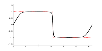
(a) $\lambda=1.6$

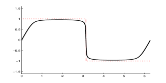
(b) $\lambda=1.1$

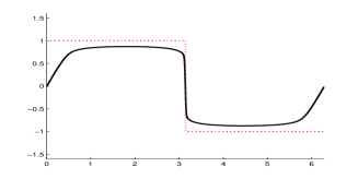
(c) $\lambda=0.6$

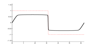
(d) $\lambda=0.1$

Figure 1. Solutions of system (7.3) with $N=256$ and $T=0.5$. The piecewise constant initial datum is $u_{0}(x)=\text{sgn}(\pi-x)$.

Proposition 7.1.

(7.2) $$G^{\pi_{\lambda}}(\xi)=\left\{\begin{split}&-C_{\lambda}\,|\xi|^{\lambda}&\text{\emph{for} $d=1$,}\\ &-C_{\lambda}\,|\xi|^{\lambda}\int_{|y|=1}\mathrm{d}S_{y}\,&\text{\emph{for} $d>1$,}\end{split}\right.$$

where $C_{\lambda}=2\,c_{\lambda}\,\lambda^{-1}\int_{0}^{\infty}x^{-\lambda}\sin x\,\mathrm{d}x>0$ and $\int_{|y|=1}\mathrm{d}S_{y}=2\pi^{d/2}\,\Gamma^{-1}(\frac{d}{2})$.

The proof is given at the end of this section. In the above result and in the following, $dS_{y}$ will denote the surface area measure of the unit sphere $|y|=1$. Expression (7.2) is the “Fourier symbol” of the fractional Laplace operator in our periodic setting. When $\lambda\in(0,1)$, the integral $\Theta_{\lambda}=\int_{0}^{\infty}x^{-\lambda}\sin x\,\mathrm{d}x$ is a generalized Fresnel integral [29] with value

$$\begin{split}\Theta_{\lambda}=\Gamma(1-\lambda)\sin\left(\frac{\pi(1-\lambda)}{2}\right).\end{split}$$

When $\lambda=1$, $\Theta_{\lambda}$ is a Dirichlet integral [24] and has value $\frac{\pi}{2}$. For $\lambda\in(1,2)$, the integral $\Theta_{\lambda}$ has to be evaluated numerically since explicit formulas are not available.

(a) $\lambda=1.6$

(b) $\lambda=1.1$

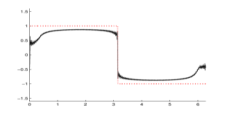
(c) $\lambda=0.6$

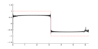
(d) $\lambda=0.1$

Figure 2. Solutions of system (7.3) with $N=256$, $T=0.5$, and $\epsilon_{N}=0$. The piecewise constant initial datum is $u_{0}(x)=\mathrm{sgn}(\pi-x)$.

Remark 7.2.

By Proposition 7.1 there is a positive constant such that

$$\begin{split}\int_{\Lambda}\mathcal{L}^{\pi_{\lambda}}[u_{N}(\cdot,t)]\,u_{N}(\cdot,t)\ \mathrm{d}x&=-C\,\sum_{|\xi|\leq N}|\xi|^{\lambda}|\hat{u}_{\xi}(t)|^{2},\end{split}$$

where right-hand side is a fractional Sobolev semi-norm [4]

$$\begin{split}\sum_{|\xi|\leq N}|\xi|^{\lambda}|\hat{u}_{\xi}(t)|^{2}=|u_{N}(\cdot,t)|^{2}_{H^{\lambda/2}(\Lambda)}.\end{split}$$

Simple energy estimates can then be used to show that the solutions of (7.1) belong to $H^{\lambda/2}(\Lambda)$, which is more regularity than what can be expected for general solutions of the pure Burgers’ equation ($\mu=0$).

We now use the SVV method (3.1) to work out some approximate solutions of the fractional Burgers’ equation (7.1) with $d=1$. Hence $f(u)=u^{2}/2$ and $\mu=\pi_{\lambda}$ in (3.1). We multiply both sides of (3.1) by $e^{-i\xi\,x}$, and integrate over $(0,2\pi)$ to obtain the following system of ODEs

(7.3) $$\begin{split}\frac{\mathrm{d}}{\mathrm{d}t}\hat{u}_{\xi}(t)+\frac{i\xi}{2}\sum_{\stackrel{{\scriptstyle|p|,|q|\leq N}}{{p+q=\xi}}}\hat{u}_{p}(t)\,\hat{u}_{q}(t)+C_{\lambda}\,|\xi|^{\lambda}\hat{u}_{\xi}(t)+\epsilon_{N}\mathbf{1}_{m_{N}\leq|\xi|\leq N}|\xi|^{2}\,\hat{Q}_{\xi}(t)\,\hat{u}_{\xi}(t)=0,\end{split}$$

where the Fourier coefficients $\hat{Q}_{\xi}$ satisfy the assumptions listed in Section 3 and are chosen as in [30] (they vary continuously between zero and one). In our simulations we have used a fourth order Runge-Kutta solver for (7.3).

The results of our numerical simulations can be found in Figure 1 and 2. The results in Figure 1 confirm the convergence of our SVV approximation (7.3) for all all values of $\lambda\in(0,2)$. In Figure 2 we have solved the (7.3) with $\epsilon_{N}=0$ (no spectral vanishing viscosity). For $\lambda>1$, convergence continues to hold, while for $\lambda<1$, convergence fails and spurious Gibbs oscillations appear. This is consistent with the theoretical results for fractional conservation laws [2, 18]: These equations admit smooth solutions for $\lambda>1$ (the strong diffusion case), while shock discontinuities may appear for $\lambda<1$ (the weak diffusion case).

Proof of Proposition 7.1.

Let us prove the case $d=1$ first. By Euler’s formula, $e^{i\xi z}=\cos(\xi z)+i\sin(\xi z)$, we find that

$$\begin{split}\int_{|z|<1}\frac{e^{i\xi z}-1-i\xi z}{|z|^{1+\lambda}}\ \mathrm{d}z&=\int_{|z|<1}\frac{\cos(\xi z)-1}{|z|^{1+\lambda}}\ \mathrm{d}z+i\int_{|z|<1}\frac{\sin(\xi z)-\xi z}{|z|^{1+\lambda}}\ \mathrm{d}z.\end{split}$$

Taylor expansions show that these integrals are finite. In fact, the $\sin$-integral is zero since the its integrand is odd. Integration by parts then leads to

$$\begin{split}\int_{|z|<1}\frac{\cos(\xi z)-1}{|z|^{1+\lambda}}\ \mathrm{d}z&=2\int_{0}^{1}\frac{\cos(\xi z)-1}{z^{1+\lambda}}\ \mathrm{d}z\\ &=-\frac{2}{\lambda z^{\lambda}}(\cos(\xi z)-1)\Big{|}_{0}^{1}-\frac{2\xi}{\lambda}\int_{0}^{1}\frac{\sin(\xi z)}{z^{\lambda}}\ \mathrm{d}z\\ &=-\frac{2}{\lambda}(\cos(\xi)-1)-\frac{2\xi}{\lambda}\int_{0}^{1}\frac{\sin(\xi z)}{z^{\lambda}}\ \mathrm{d}z.\end{split}$$

Now we consider the integral over $|z|>r$. Again the imaginary part (the sine part) is zero, and a computation like the one we performed above reveals that

$$\begin{split}\int_{|z|>1}\frac{e^{i\xi z}-1}{|z|^{1+\lambda}}\ \mathrm{d}z=\frac{2}{\lambda}(\cos(\xi)-1)-\frac{2\xi}{\lambda}\int_{1}^{\infty}\frac{\sin(\xi z)}{z^{\lambda}}\ \mathrm{d}z.\end{split}$$

Note the + sign of the cosine-term! We add these two equations and find that

$$\begin{split}G^{\pi_{\lambda}}(\xi)=-\frac{2\xi c_{\lambda}}{\lambda}\int_{0}^{\infty}\frac{\sin(\xi z)}{z^{\lambda}}\ \mathrm{d}z.\end{split}$$

The integral $\int_{0}^{\infty}z^{-\lambda}\sin(\xi z)\,\mathrm{d}z$ is finite and positive for all $\lambda\in(0,2)$ (cf. [16] for details). Whenever $\xi>0$, we can use the change of variable $\xi z\rightarrow x$ to deduce that

$$\begin{split}\int_{0}^{\infty}\frac{\sin(\xi z)}{z^{\lambda}}\ \mathrm{d}z=\xi^{\lambda-1}\int_{0}^{\infty}\frac{\sin x}{x^{\lambda}}\ \mathrm{d}x\end{split}$$

and thus

$$\begin{split}G^{\pi_{\lambda}}(\xi)&=-\frac{2c_{\lambda}}{\lambda}\,\xi^{\lambda}\int_{0}^{\infty}\frac{\sin x}{x^{\lambda}}\ \mathrm{d}x.\end{split}$$

When $\xi<0$, we use the relation $\sin(-\xi x)=-\sin(\xi x)$ to obtain

$$\begin{split}G^{\pi_{\lambda}}(\xi)&=-\frac{2c_{\lambda}}{\lambda}\,|\xi|^{\lambda}\int_{0}^{\infty}\frac{\sin x}{x^{\lambda}}\ \mathrm{d}x,\end{split}$$

and the conclusion for $d=1$ follows.

When $d>1$ we use polar coordinates $x=ry$ for $r>0$ and $|y|=1$, and we find that

$$\begin{split}\int_{|z|<1}\frac{e^{i\xi\cdot z}-1-i\xi\cdot z}{|z|^{d+\lambda}}\ \mathrm{d}z&=\int_{|y|=1}\int_{0}^{1}\frac{\cos(\xi\cdot y\,r)-1}{r^{d+\lambda}}\ r^{d-1}\mathrm{d}r\,\mathrm{d}S_{y},\\ \int_{|z|>1}\frac{e^{i\xi\cdot z}-1}{|z|^{d+\lambda}}\ \mathrm{d}z&=\int_{|y|=1}\int_{1}^{\infty}\frac{\cos(\xi\cdot y\,r)-1}{r^{1+\lambda}}\ \mathrm{d}r\,\mathrm{d}S_{y}.\end{split}$$

Proceeding as in the $d=1$ case for the $r$-integral with $y$ fixed, we find that

$$\begin{split}G^{\pi_{\lambda}}(\xi)&=-\frac{2c_{\lambda}}{\lambda}\int_{|y|=1}|\xi\cdot y|^{\lambda}\ \mathrm{d}S_{y}\int_{0}^{\infty}\frac{\sin x}{x^{\lambda}}\ \mathrm{d}x\\ &=-\frac{2c_{\lambda}}{\lambda}\,|\xi|^{\lambda}\int_{|y|=1}\left|\frac{\xi}{|\xi|}\cdot y\right|^{\lambda}\ \mathrm{d}S_{y}\int_{0}^{\infty}\frac{\sin x}{x^{\lambda}}\ \mathrm{d}x.\end{split}$$

By symmetry, the value of the $y$-integral is the same for any $\xi$. Therefore,

$$\begin{split}\int_{|y|=1}\left|\frac{\xi}{|\xi|}\cdot y\right|^{\lambda}\ \mathrm{d}S_{y}=\int_{|y|=1}\left|y\cdot y\right|^{\lambda}\ \mathrm{d}S_{y}=\int_{|y|=1}\mathrm{d}S_{y}.\end{split}$$

The proof for the case $d>1$ is now complete. ∎

8. Extension to asymmetric measures $\mu$

In this section we show how to modify the arguments of the previous sections to obtain results for a large class of non-symmetric measures $\mu$ including all the Lévy measures used in finance. A careful look at the previous arguments shows that symmetry of $\mu$ is used for the sole purpose of having a sign of the fractional term in the energy inequality (see (4.14)) in order to prove Theorems 4.1 and 4.2. This fractional term is

(8.1) $$\begin{split}\iint_{D_{T}}\mathcal{L}^{\mu}[u_{N}]\,\partial_{x}^{2\alpha}u_{N}\ \mathrm{d}x\,\mathrm{d}t=\sum_{|\xi|\leq N}G^{\mu}(\xi)\,|\xi^{\alpha}|^{2}\int_{0}^{T}|\hat{u}_{\xi}(t)|^{2}\ \mathrm{d}t,\end{split}$$

and it is non-positive when $\mu$ is symmetric. In the general case the sign of the fractional term (8.1) is unknown, but everything still works if we assume that

$$\mu=\mu_{s}+\mu_{n},$$

for $\mu_{s},\mu_{n}$ satisfying (1.6) (i.e. we assume (1.5) and (1.6)). Note that in this case, we may split the weights in (3.4) into their symmetric and non-symmetric parts,

$$G^{\mu}(\xi)=G^{\mu_{s}}(\xi)+G^{\mu_{n}}(\xi),$$

where $G^{\mu_{s}}(\xi)$ is again real and non-positive, and by (1.6),

(8.2) $$\begin{split}|G^{\mu_{n}}(\xi)|=\bigg{|}\int_{|z|>0}e^{i\xi\cdot z}-1-i\xi\cdot z\,\mathbf{1}_{|z|<1}\ \mathrm{d}\mu_{n}(z)\bigg{|}\leq C_{n}\Big{(}1+|\xi|\Big{)}.\end{split}$$

The main result of this section is the following:

Theorem 8.1.

(Convergence with rate) Let $(\mathbf{A}.1)$–$(\mathbf{A}.9)$, (1.5) and (1.6) hold, $u_{N}$ be the solution of the SVV method (3.1), and $u$ be an entropy solution of (1.1). Then,

$$\begin{split}\|u(\cdot,T)-u_{N}(\cdot,T)\|_{L^{1}(\Lambda)}\leq C\,\sqrt{\epsilon_{N}}.\end{split}$$

To prove this result, we have to modify the arguments of the previous sections. In view of the above discussion the key result to obtain is a version of Theorem 4.1 for measures $\mu$ satisfying (1.5) and (1.6):

Theorem 8.2.

Assume (A.1)–(A.7), (1.5), (1.6) hold, and let $u_{N}$ be the solution of the SVV approximation (3.1). Then there exists a constant $\tilde{\mathcal{B}}_{s}$ (proportional to $1+\Pi_{k=1}^{s}\mathcal{K}_{s}$ for $s\geq 1$ and to $\|u_{N}\|_{L^{\infty}}$ for $s=0$, see Theorem 4.1) such that

$$\begin{split}&\epsilon^{s}_{N}\|\partial_{x}^{s}u_{N}(\cdot,t)\|_{L^{2}(\Lambda)}+\epsilon_{N}^{s+\frac{1}{2}}\|\partial_{x}^{s+1}u_{N}\|_{L^{2}(D_{T})}\leq\tilde{\mathcal{B}}_{s}+4\epsilon_{N}^{s}\|\partial_{x}^{s}u_{N}(\cdot,0)\|_{L^{2}(\Lambda)}.\end{split}$$

We prove this result at the end of this section. Now if we also assume that (A.8) and (A.9) hold, then it easily follows that Theorem 4.2 still holds if we replace $\mathcal{B}_{s}$ by $\tilde{\mathcal{B}}_{s}$. At this point the reader may easily check that all the other results also hold if we everywhere replace $\mathcal{B}_{s}$ by $\tilde{\mathcal{B}}_{s}$ – and hence Theorem 8.1 follows.

Remark 8.3.

A Lévy measure $\mu$ defined by

$$\mathrm{d}\mu=g(z)\,\mathrm{d}\pi_{\lambda}(z),$$

(see (1.4)) can be written as $\mu=\mu_{s}+\mu_{n}$ where

$$\mathrm{d}\mu_{s}=g(z)\wedge g(-z)\,\mathrm{d}\pi_{\lambda}\quad\text{and}\quad\mathrm{d}\mu_{n}=[g(z)-g(z)\wedge g(-z)]\,\mathrm{d}\pi_{\lambda}.$$

Note that $\mu_{s},\mu_{n}\geq 0$, $\mu_{s}$ is symmetric, and that $\mu_{n}$ satisfies the integrability condition in (1.6) if $g$ is locally Lipschitz: Let $g_{n}(z)=g(z)-g(z)\wedge g(-z)$ and note that $g_{n}(0)=0$, hence $g_{n}(z)=|g_{n}(z)-g_{n}(0)|\leq C\,|z|$ for $|z|<1$.

We now show how to modify the proof of Theorem 4.1 to prove Theorem 8.2.

Proof of Theorem 8.2.

Once again we use the shorthand $\|\cdot\|$ instead of $\|\cdot\|_{L^{2}(\Lambda)}$, and rewrite the SVV approximation (3.1) as in (4.9) and (4.10). Note that (5.1) and (5.2) holds for general measures $\mu$, so we find that

$$\int_{\Lambda}\mathcal{L}^{\mu}[u_{N}]\,u_{N}\ \mathrm{d}x\leq\int_{\Lambda}\mathcal{L}^{\mu}[u^{2}_{N}]\ \mathrm{d}x=0.$$

Hence, spatial integration of (4.10) against $u_{N}$ yields

$$\begin{split}&\frac{1}{2}\frac{\mathrm{d}}{\mathrm{d}t}\|u_{N}\|^{2}+\epsilon_{N}\,\|\partial_{x}u_{N}\|^{2}\\ &\leq\epsilon_{N}\|u_{N}\|\bigg{\|}\sum_{j,k=1}^{d}\partial_{j}\partial_{k}R_{N}^{j,k}\ast u_{N}\bigg{\|}+\sum_{j=1}^{d}\|\partial_{j}u_{N}\|\|(I-P_{N})f_{j}(u_{N})\|,\end{split}$$

and the conclusion in the case $s=0$ follows exactly as in the first part of the proof of Theorem 4.1.

Now let $s>0$, and note that by (8.2) and Young’s inequality,

$$\begin{split}\int_{\Lambda}\partial_{x}^{2\alpha}u_{N}\ \mathcal{L}^{\mu_{n}}[u_{N}]\ \mathrm{d}x&=\sum_{|\xi|\leq N}(-i\xi)^{2\alpha}\,G^{\mu_{n}}(\xi)\,|\hat{u}_{\xi}(t)|^{2}\\ &\leq\sum_{|\xi|\leq N}C_{n}\Big{(}1+|\xi|\Big{)}|\xi^{\alpha}|^{2}\,|\hat{u}_{\xi}(t)|^{2}\\ &\leq\sum_{|\xi|\leq N}\left(C_{n}+\frac{\epsilon_{N}}{4}\,|\xi|^{2}+\frac{C_{n}^{2}}{\epsilon_{N}}\right)|\xi^{\alpha}|^{2}|\hat{u}_{\xi}(t)|^{2}.\end{split}$$

If we take this into account and perform spatial integration of (4.9) against $\partial_{x}^{2\alpha}u_{N}$ for some multi-index $\alpha$, we find the following modified version of (4.11),

$$\begin{split}&\frac{1}{2}\frac{\mathrm{d}}{\mathrm{d}t}\|\partial_{x}^{\alpha}u_{N}\|^{2}-\sum_{|\xi|\leq N}G^{\mu_{s}}(\xi)|\xi^{\alpha}|^{2}|\hat{u}_{\xi}(t)|^{2}+\frac{3\,\epsilon_{N}}{4}\|\partial^{\alpha}_{x}\partial_{x}u_{N}\|^{2}\\ &\leq\epsilon_{N}\|\partial_{x}^{\alpha}u_{N}\|\bigg{\|}\sum_{j,k=1}^{d}\partial_{j}\partial_{k}R_{N}^{j,k}\ast\partial_{x}^{\alpha}u_{N}\bigg{\|}\\ &\quad+\|\partial_{x}^{\alpha}\partial_{x}u_{N}\|\|\partial_{x}^{|\alpha|-1}\partial_{x}\cdot P_{N}f(u_{N})\|+\frac{2\,C_{n}^{2}}{\epsilon_{N}}\|\partial_{x}^{\alpha}u_{N}\|^{2}.\end{split}$$

As in the proof of Theorem 4.1, we now use (3.8) and Young’s inequality to bound the first and second term on the right hand side. The result is that

$$\begin{split}&\frac{1}{2}\frac{\mathrm{d}}{\mathrm{d}t}\|\partial_{x}^{\alpha}u_{N}\|^{2}-\sum_{|\xi|\leq N}G^{\mu_{s}}(\xi)|\xi^{\alpha}|^{2}|\hat{u}_{\xi}(t)|^{2}+\frac{\epsilon_{N}}{2}\|\partial^{\alpha}_{x}\partial_{x}u_{N}\|^{2}\\ &\qquad\qquad\qquad\qquad\qquad\leq C\,\|\partial_{x}^{\alpha}u_{N}\|^{2}+\frac{1}{\epsilon_{N}}\|\partial_{x}^{|\alpha|}P_{N}f(u_{N})\|^{2}+\frac{2\,C_{n}^{2}}{\epsilon_{N}}\|\partial_{x}^{\alpha}u_{N}\|^{2}.\end{split}$$

Now we sum over all $|\alpha|=s$ to find that

$$\begin{split}&\frac{1}{2}\frac{\mathrm{d}}{\mathrm{d}t}\|\partial_{x}^{s}u_{N}\|^{2}-\sum_{|\alpha|=s}\sum_{|\xi|\leq N}G^{\mu_{s}}(\xi)|\xi^{\alpha}|^{2}|\hat{u}_{\xi}(t)|^{2}+\frac{\epsilon_{N}}{2}\|\partial^{s+1}_{x}u_{N}\|^{2}\\ &\qquad\qquad\qquad\qquad\qquad\leq C\,\|\partial_{x}^{s}u_{N}\|^{2}+\frac{d^{s}}{\epsilon_{N}}\|\partial_{x}^{s}P_{N}f(u_{N})\|^{2}+\frac{2\,C_{n}^{2}}{\epsilon_{N}}\|\partial_{x}^{s}u_{N}\|^{2}.\end{split}$$

Thanks to (4.1) and (4.2),

$$\begin{split}\|\partial_{x}^{s}P_{N}f(u_{N})\|\leq\mathcal{K}_{s}\,\|\partial_{x}^{s}u_{N}\|+\frac{\mathcal{K}_{s+1}}{N}\,\|\partial_{x}^{s+1}u_{N}\|,\end{split}$$

and hence

$$\begin{split}\frac{1}{2}\frac{\mathrm{d}}{\mathrm{d}t}\|\partial_{x}^{s}u_{N}\|^{2}-\sum_{|\alpha|=s}\sum_{|\xi|\leq N}G^{\mu_{s}}(\xi)|\xi^{\alpha}|^{2}|\hat{u}_{\xi}(t)|^{2}+\left(\frac{\epsilon_{N}}{2}-\frac{2d^{s}\mathcal{K}^{2}_{s+1}}{N^{2}\epsilon_{N}}\right)\|\partial_{x}^{s+1}u_{N}\|^{2}\\ \leq\left(C+\frac{2\,C_{n}^{2}+2d^{s}\mathcal{K}_{s}^{2}}{\epsilon_{N}}\right)\,\|\partial_{x}^{s}u_{N}\|^{2}\leq\frac{2\,C_{n}^{2}+3d^{s}\mathcal{K}_{s}^{2}}{\epsilon_{N}}\,\|\partial_{x}^{s}u_{N}\|^{2},\end{split}$$

where the last inequality holds for $N$ big enough.

To conclude, we use (A.7) to obtain

$$\begin{split}\frac{1}{2}\|\partial_{x}^{s}u_{N}(\cdot,t)\|^{2}-\sum_{|\alpha|=s}\sum_{|\xi|\leq N}G^{\mu_{s}}(\xi)|\xi^{\alpha}|^{2}\int_{0}^{t}|\hat{u}_{\xi}(\tau)|^{2}\,\mathrm{d}\tau+\frac{\epsilon_{N}}{4}\|\partial_{x}^{s+1}u_{N}\|^{2}_{L^{2}(D_{T})}\\ \leq\frac{2\,C_{n}^{2}+3d^{s}\mathcal{K}_{s}^{2}}{\epsilon_{N}}\,\|\partial_{x}^{s}u_{N}\|^{2}_{L^{2}(D_{T})}+\frac{1}{2}\|\partial_{x}^{s}u_{N}(\cdot,0)\|^{2}.\end{split}$$

The proof is now complete since by induction on $s$,

$$\begin{split}\|\partial_{x}^{s}u_{N}\|^{2}_{L^{2}(D_{T})}\leq C\,\tilde{\mathcal{B}}^{2}_{s-1}\epsilon_{N}^{-(2s-1)}.\end{split}$$

∎

Appendix A Proof of Theorem 2.2

Let us take $\varphi=\psi(x,y,t,s)$, $u=u(x,t)$ and $v=v(y,s)$. We set $k=v(y,s)$ in the entropy inequality for $u(x,t)$, and integrate over all $(y,s)\in Q_{T}$ to obtain

$$\begin{split}&\iint_{D_{T}}\iint_{D_{T}}\eta(u(x,t),v(y,s))\,\partial_{t}\psi(x,y,t,s)\\ &\qquad\qquad+q(u(x,t),v(y,s))\cdot\partial_{x}\psi(x,y,t,s)\\ &\qquad\qquad+\eta(u(x,t),v(y,s))\,\mathcal{L}_{r}^{\ast,\mu}[\psi(\cdot,y,t,s)](x)\\ &\qquad\qquad+\eta^{\prime}(u(x,t),v(y,s))\,\mathcal{L}^{\mu,r}[u(\cdot,t)](x)\,\psi(x,y,t,s)\\ &\qquad\qquad+\eta(u(x,t),v(y,s))\,\gamma_{\mu}^{r}\cdot\partial_{x}\psi(x,y,t,s)\ \mathrm{d}x\,\mathrm{d}t\,\mathrm{d}y\,\mathrm{d}s\geq 0.\end{split}$$

In the entropy inequality for $v(y,s)$, we set $k=u(x,t)$ and integrate with respect to $(x,t)$ to find that

$$\begin{split}&\iint_{D_{T}}\iint_{D_{T}}\eta(u(x,t),v(y,s))\,\partial_{s}\psi(x,y,t,s)\\ &\qquad\qquad+q(u(x,t),v(y,s))\cdot\partial_{y}\psi(x,y,t,s)\\ &\qquad\qquad+\eta(u(x,t),v(y,s))\,\mathcal{L}_{r}^{\ast,\mu}[\psi(x,\cdot,t,s)](y)\\ &\qquad\qquad-\eta^{\prime}(u(x,t),v(y,s))\,\mathcal{L}^{\mu,r}[v(\cdot,s)](y)\,\psi(x,y,t,s)\\ &\qquad\qquad+\eta(u(x,t),v(y,s))\,\gamma_{\mu}^{r}\cdot\partial_{y}\psi(x,y,t,s)\ \mathrm{d}y\,\mathrm{d}s\,\mathrm{d}x\,\mathrm{d}t\geq 0.\end{split}$$

In the following we need the $\mathbb{R}^{2d}$-operators

$$\begin{split}\tilde{}\mathcal{L}^{\mu,r}[\phi(\cdot,\cdot)](x,y)&=\int_{|z|>r}\phi(x+z,y+z)-\phi(x,y)\ \mathrm{d}\mu(z),\\ \tilde{}\mathcal{L}^{\ast,\mu,r}[\phi(\cdot,\cdot)](x,y)&=\int_{|z|>r}\phi(x-z,y-z)-\phi(x,y)\ \mathrm{d}\mu(z).\end{split}$$

With these definitions in mind, we add the two inequalities above and change the order of integration to find that

$$\begin{split}&\iint_{D_{T}}\iint_{D_{T}}\eta(u(x,t),v(y,s))\,(\partial_{t}+\partial_{s})\psi(x,y,t,s)\\ &\qquad\qquad+q(u(x,t),v(y,s))\cdot(\partial_{x}+\partial_{y})\psi(x,y,t,s)\\ &\qquad\qquad+\eta(u(x,t),v(y,s))\,\mathcal{L}_{r}^{\ast,\mu}[\psi(\cdot,y,t,s)](x)\\ &\qquad\qquad+\eta(u(x,t),v(y,s))\,\mathcal{L}_{r}^{\ast,\mu}[\psi(x,\cdot,t,s)](y)\\ &\qquad\qquad+\eta^{\prime}(u(x,t),v(y,s))\,\tilde{}\mathcal{L}^{\mu,r}[u(\cdot,t)-v(\cdot,s)](x,y)\,\psi(x,y,t,s)\\ &\qquad\qquad+\eta(u(x,t),v(y,s))\,\gamma_{\mu}^{r}\cdot(\partial_{x}+\partial_{y})\psi(x,y,t,s)\ \mathrm{d}w\geq 0.\end{split}$$

Here and in the following we use the shorthand $\mathrm{d}w=\mathrm{d}x\,\mathrm{d}t\,\mathrm{d}y\,\mathrm{d}s$. Note that

$$\begin{split}\eta^{\prime}(u(x,t),v(y,s))\,\tilde{}\mathcal{L}^{\mu,r}[u(\cdot,t)-v(\cdot,s)](x,y)\leq\tilde{}\mathcal{L}^{\mu,r}[\eta(u(\cdot,t),v(\cdot,s))](x,y).\end{split}$$

Moreover, using the change of variables $(x,y)\rightarrow(x-z,y-z)$,

$$\begin{split}&\iint_{D_{T}}\iint_{D_{T}}\psi(x,y,t,s)\,\tilde{}\mathcal{L}^{\mu,r}[\eta(u(\cdot,t),v(\cdot,s))](x,y)\ \mathrm{d}w\\ &=\int_{|z|>r}\int_{0}^{T}\int_{z+\Lambda}\int_{0}^{T}\int_{z+\Lambda}\eta(u(x,t),v(y,s))\,\psi(x-z,y-z,t,s)\ \mathrm{d}w\,\mathrm{d}\mu(z)\\ &\quad-\int_{|z|>r}\iint_{D_{T}}\iint_{D_{T}}\eta(u(x,t),v(y,s))\,\psi(x,y,t,s)\ \mathrm{d}w\,\mathrm{d}\mu(z),\end{split}$$

which by periodicity and the definition of $\tilde{}\mathcal{L}^{\ast,\mu,r}$ equals to

$$\begin{split}&\int_{|z|>r}\int_{0}^{T}\int_{\Lambda}\int_{0}^{T}\int_{\Lambda}\eta(u(x,t),v(y,s))\,\psi(x-z,y-z,t,s)\ \mathrm{d}w\,\mathrm{d}\mu(z)\\ &\quad-\int_{|z|>r}\iint_{D_{T}}\iint_{D_{T}}\eta(u(x,t),v(y,s))\,\psi(x,y,t,s)\ \mathrm{d}w\,\mathrm{d}\mu(z)\\ &=\iint_{D_{T}}\iint_{D_{T}}\eta(u(x,t),v(y,s))\,\tilde{}\mathcal{L}^{\ast,\mu,r}[\psi(\cdot,\cdot,t,s)](x,y)\ \mathrm{d}w.\end{split}$$

Therefore we have proved so far that

$$\begin{split}&\iint_{D_{T}}\iint_{D_{T}}\eta(u(x,t),v(y,s))\,(\partial_{t}+\partial_{s})\psi(x,y,t,s)\\ &\qquad\qquad+q(u(x,t),v(y,s))\cdot(\partial_{x}+\partial_{y})\psi(x,y,t,s)\\ &\qquad\qquad+\eta(u(x,t),v(y,s))\,\mathcal{L}_{r}^{\ast,\mu}[\psi(\cdot,y,t,s)](x)\\ &\qquad\qquad+\eta(u(x,t),v(y,s))\,\mathcal{L}_{r}^{\ast,\mu}[\psi(x,\cdot,t,s)](y)\\ &\qquad\qquad+\eta(u(x,t),v(y,s))\,\tilde{}\mathcal{L}^{\ast,\mu,r}[\psi(\cdot,\cdot,t,s)](x,y)\\ &\qquad\qquad+\eta(u(x,t),v(y,s))\,\gamma_{\mu}^{r}\cdot(\partial_{x}+\partial_{y})\psi(x,y,t,s)\ \mathrm{d}w\geq 0.\end{split}$$

We now send $r\rightarrow 0$, remembering the definition of $\gamma_{\mu}^{r}$ and defining

$$\begin{split}&\tilde{}\mathcal{L}^{\ast,\mu}[\phi(\cdot,\cdot)](x,y)\\ &=\int_{|z|>0}\phi(x-z,y-z)-\phi(x,y)+z\cdot(\partial_{x}+\partial_{y})\phi(x,y)\,\mathbf{1}_{|z|<1}\ \mathrm{d}\mu(z).\end{split}$$

The result is

(A.1) $$\begin{split}&\iint_{D_{T}}\iint_{D_{T}}\eta(u(x,t),v(y,s))\,(\partial_{t}+\partial_{s})\psi(x,y,t,s)\\ &\qquad\qquad+q(u(x,t),v(y,s))\cdot(\partial_{x}+\partial_{y})\psi(x,y,t,s)\\ &\qquad\qquad+\eta(u(x,t),v(y,s))\,\tilde{}\mathcal{L}^{\ast,\mu}[\psi(\cdot,\cdot,t,s)](x,y)\ \mathrm{d}w\geq 0.\end{split}$$

To conclude, we show how to derive the $L^{1}$-contraction (2.2) from this inequality by choosing the test function $\psi$ as

(A.2) $$\begin{split}\psi(x,y,t,s)=\hat{\omega}_{\rho}\left(\frac{x-y}{2}\right)\omega_{\delta}\left(\frac{t-s}{2}\right)\phi(t),\quad\rho,\delta>0,\end{split}$$

where $\omega_{\delta}(\tau)=\frac{1}{\delta}\,\omega(\frac{\tau}{\delta})$ for a nonnegative $\omega\in C_{c}^{\infty}(\mathbb{R})$ satisfying

$$\begin{split}\omega(-\tau)=\omega(\tau),\quad\omega(\tau)=0\text{ for all $|\tau|\geq 1$,$\quad$and}\quad\int_{\mathbb{R}}\omega(\tau)\,\mathrm{d}\tau=1,\end{split}$$

while $\hat{\omega}_{\rho}(x)=\bar{\omega}_{\rho}(x_{1})\cdots\bar{\omega}_{\rho}(x_{d})$ with $\bar{\omega}_{\rho}(\cdot)$ such that

$$\begin{split}\bar{\omega}_{\rho}(\tau)=\sum_{k\in\mathbb{Z}}\omega_{\rho}(\tau+2\pi k).\end{split}$$

Note that $\hat{\omega}_{\rho}$ is periodic in each coordinate direction. By a direct computation,

$$\begin{split}(\partial_{t}+\partial_{s})\psi(x,y,t,s)&=\hat{\omega}_{\rho}\left(\frac{x-y}{2}\right)\omega_{\delta}\left(\frac{t-s}{2}\right)\,\phi^{\prime}(t),\\ (\partial_{x}+\partial_{y})\psi(x,y,t,s)&=0,\\ \tilde{}\mathcal{L}^{\ast}[\psi(\cdot,\cdot,t,s)](x,y)&=0.\end{split}$$

Thus, with this test function $\psi$ at hand, inequality (A.1) becomes

(A.3) $$\begin{split}&\iint_{D_{T}}|u(x,t)-v(y,s)|\,\hat{\omega}_{\rho}\left(\frac{x-y}{2}\right)\omega_{\delta}\left(\frac{t-s}{2}\right)\,\phi^{\prime}(t)\ \mathrm{d}w\geq 0.\end{split}$$

We then go to the limit as $(\rho,\delta)\rightarrow 0$ to find that

(A.4) $$\begin{split}\iint_{D_{T}}|u(x,t)-v(x,t)|\,\phi^{\prime}(t)\ \mathrm{d}x\,\mathrm{d}t\geq 0.\end{split}$$

To conclude the proof we now take $\phi=\chi_{\mu}$ for

(A.5) $$\chi_{\mu}(t) =\int_{-\infty}^{t}(\omega_{\mu}(\tau-t_{1})-\omega_{\mu}(\tau-t_{2}))\ \mathrm{d}\tau,\qquad 0<t_{1}<t_{2}<T.$$

Loosely speaking, the function $\chi_{\mu}$ is a smooth approximation of the indicator function $\mathbf{1}_{(t_{1},t_{2})}$ which is zero near $t=0$ and $t=T$ for $\mu>0$ small. Since

$$\chi_{\mu}^{\prime}(t)=\omega_{\mu}(t-t_{1})-\omega_{\mu}(t-t_{2}),$$

inequality (A.4) reduces to

$$\iint_{Q_{T}}|u(x,t)-v(x,t)|\,\omega_{\mu}(t-t_{2})\ \mathrm{d}t\,\mathrm{d}x\leq\iint_{Q_{T}}|u(x,t)-v(x,t)|\,\omega_{\mu}(t-t_{1})\ \mathrm{d}t\,\mathrm{d}x.$$

By the integrability of $u$ and $v$ and Fubini’s theorem, the function

$$\Phi(t)=\int_{\Lambda}|u(x,t)-v(x,t)|\ \mathrm{d}x\in L^{1}(0,T),$$

and we may write the above inequality as a convolution

$$\Phi*\omega_{\mu}(t_{2})\leq\Phi*\omega_{\mu}(t_{1}).$$

By standard properties of convolutions, $\Phi*\omega_{\mu}(t)\rightarrow\Phi(t)$ a.e. $t$ as $\mu\rightarrow 0$. Hence,

$$\|(u-v)(\cdot,t_{2})\|_{L^{1}(\Lambda)}\leq\|(u-v)(\cdot,t_{1})\|_{L^{1}(\Lambda)}\quad\text{for a.e.~{}$t_{1},t_{2}\in(0,T)$}.$$

Finally, the theorem follows from renaming $t_{2}$ and using part iii) in Definition 2.1 to send $t_{1}\rightarrow 0$.

Appendix B Proof of Theorem 2.4

The vanishing viscosity problem (2.3) has a unique classical solution $u_{\epsilon}$ for $\varepsilon>0$, see Remark 2.6. If we multiply (2.3) by $\eta^{\prime}(u_{\epsilon})$ for any smooth convex function $\eta$, use standard manipulations on the conservation law part combined with the inequalities

$$\eta^{\prime}(u_{\epsilon})\mathcal{L}^{\mu}[u_{\epsilon}]=\eta^{\prime}(u_{\epsilon})\bigg{(}\mathcal{L}^{\mu}_{r}[u_{\epsilon}]+\mathcal{L}^{\mu,r}[u_{\epsilon}]\bigg{)}\leq\mathcal{L}_{r}^{\mu}[\eta(u_{\epsilon})]+\eta^{\prime}(u_{\epsilon})\mathcal{L}^{\mu,r}[u_{\epsilon}],$$

$$\eta^{\prime}(u_{\epsilon})\,\Delta u_{\epsilon}=\Delta\eta(u_{\epsilon})-\epsilon\,\eta^{\prime\prime}(u_{\epsilon})|\partial_{x}u_{\epsilon}|^{2}\leq\Delta\eta(u_{\epsilon}),$$

we find, after integration against any nonnegative test function $\phi$, that $u_{\epsilon}$ satisfies the (entropy) inequality

$$\begin{split}&\iint_{D_{T}}\eta(u_{\epsilon},k)\,\partial_{t}\varphi+q(u_{\epsilon},k)\cdot\partial_{x}\varphi+\eta(u_{\epsilon},k)\,\mathcal{L}_{r}^{\ast,\mu}[\varphi]+\eta^{\prime}(u_{\epsilon},k)\,\mathcal{L}^{\mu,r}[u_{\epsilon}]\\ &\qquad\qquad\qquad\qquad\qquad\qquad+\eta(u_{\epsilon},k)\,\gamma_{\mu}^{r}\cdot\partial_{x}\varphi+\epsilon\,\eta(u_{\epsilon},k)\,\Delta\varphi\ \mathrm{d}x\,\mathrm{d}t\geq 0.\end{split}$$

From this inequality we proceed as in the proof of the $L^{1}$-contraction (Theorem 2.2). We take $u=u(x,t)$, $u_{\epsilon}=u_{\epsilon}(y,s)$, and find the inequalities

$$\begin{split}&\iint_{D_{T}}\iint_{D_{T}}\eta(u(x,t),u_{\epsilon}(y,s))\,\partial_{t}\psi(x,y,t,s)\\ &\qquad\qquad+q(u(x,t),u_{\epsilon}(y,s))\cdot\partial_{x}\psi(x,y,t,s)\\ &\qquad\qquad+\eta(u(x,t),u_{\epsilon}(y,s))\,\mathcal{L}_{r}^{\ast,\mu}[\psi(\cdot,y,t,s)](x)\\ &\qquad\qquad+\eta^{\prime}(u(x,t),u_{\epsilon}(y,s))\,\mathcal{L}^{\mu,r}[u(\cdot,t)](x)\,\psi(x,y,t,s)\\ &\qquad\qquad+\eta(u(x,t),u_{\epsilon}(y,s))\,\gamma_{\mu}^{r}\cdot\partial_{x}\psi(x,y,t,s)\ \mathrm{d}w\geq 0.\end{split}$$

and

$$\begin{split}&\iint_{D_{T}}\iint_{D_{T}}\eta(u(x,t),u_{\epsilon}(y,s))\,\partial_{s}\psi(x,y,t,s)\\ &\qquad\qquad+q(u(x,t),u_{\epsilon}(y,s))\cdot\partial_{y}\psi(x,y,t,s)\\ &\qquad\qquad+\eta(u(x,t),u_{\epsilon}(y,s))\,\mathcal{L}_{r}^{\ast,\mu}[\psi(x,\cdot,t,s)](y)\\ &\qquad\qquad-\eta^{\prime}(u(x,t),u_{\epsilon}(y,s))\,\mathcal{L}^{\mu,r}[u_{\epsilon}(\cdot,s)](y)\,\psi(x,y,t,s)\\ &\qquad\qquad+\eta(u(x,t),u_{\epsilon}(y,s))\,\gamma_{\mu}^{r}\cdot\partial_{y}\psi(x,y,t,s)\ \mathrm{d}w\\ &\qquad\qquad+\epsilon\,\eta(u(x,t),u_{\epsilon}(y,s))\,\Delta_{y}\psi(x,y,t,s)\ \mathrm{d}w\geq 0.\end{split}$$

As in the proof of Theorem 2.2, we add and manipulate these to get (see (A.1))

$$\begin{split}&\iint_{D_{T}}\iint_{D_{T}}\eta(u(x,t),u_{\epsilon}(y,s))\,(\partial_{t}+\partial_{s})\psi(x,y,t,s)\\ &\qquad\qquad+q(u(x,t),u_{\epsilon}(y,s))\cdot(\partial_{x}+\partial_{y})\psi(x,y,t,s)\\ &\qquad\qquad+\eta(u(x,t),u_{\epsilon}(y,s))\,\tilde{\mathcal{L}}^{\ast,\mu}[\psi(\cdot,\cdot,t,s)](x,y)\\ &\qquad\qquad+\epsilon\,\eta(u(x,t),u_{\epsilon}(y,s))\,\Delta_{y}\psi(x,y,t,s)\ \mathrm{d}w\geq 0.\end{split}$$

We now take the test function $\psi$ as in (A.2) and find that (see (A.3))

(B.1) $$\begin{split}&-\iint_{D_{T}}\iint_{D_{T}}|u(x,t)-v(y,s)|\,\hat{\omega}_{\rho}\left(\frac{x-y}{2}\right)\omega_{\delta}\left(\frac{t-s}{2}\right)\,\phi^{\prime}(t)\ \mathrm{d}w\\ &\qquad\qquad\qquad\qquad\leq\epsilon\iint_{D_{T}}\iint_{D_{T}}\eta(u(x,t),u_{\epsilon}(y,s))\,\Delta_{y}\psi(x,y,t,s)\ \mathrm{d}w.\end{split}$$

After an integration by parts, the right-hand side (R.H.S.) is bounded by

$$\begin{split}\mathrm{R.H.S.}&\leq\epsilon\iint_{D_{T}}\iint_{D_{T}}\Big{|}\partial_{y}|u(x,t)-u_{\epsilon}(y,s)|\Big{|}\Big{|}\partial_{y}\psi(x,y,t,s)\Big{|}\,\mathrm{d}w\\ &\leq\epsilon\iint_{D_{T}}\iint_{D_{T}}|\partial_{y}u_{\epsilon}(y,s)|\left|\partial_{y}\psi(x,y,t,s)\right|\,\mathrm{d}w\\ &\leq CT\,|u_{0}|_{BV(\Lambda)}\frac{\epsilon}{\rho},\end{split}$$

where the last inequality is a consequence of the estimate $|u_{\varepsilon}(\cdot,t)|_{BV(\Lambda)}\leq|u_{0}|_{BV(\Lambda)}$ and (A.2).

To estimate the left hand side (L.H.S.) of (B.1), note that

$$\begin{split}&-|u_{\epsilon}(y,s)-u(x,t)|\phi^{\prime}(t)\\ &\geq-|u_{\epsilon}(x,t)-u(x,t)|\phi^{\prime}(t)-|u_{\epsilon}(x,s)-u_{\epsilon}(x,t)||\phi^{\prime}(t)|-|u_{\epsilon}(y,s)-u_{\epsilon}(x,s)||\phi^{\prime}(t)|,\end{split}$$

and that

$$\begin{split}\iint_{D_{T}}\iint_{D_{T}}|u_{\epsilon}(x,s)-u_{\epsilon}(x,t)|\,\hat{\omega}_{\rho}\left(\frac{x-y}{2}\right)\omega_{\delta}\left(\frac{t-s}{2}\right)\,|\phi^{\prime}(t)|\ \mathrm{d}w\stackrel{{\scriptstyle\delta\rightarrow 0}}{{\longrightarrow}}0\end{split}$$

and

$$\begin{split}&\iint_{D_{T}}\iint_{D_{T}}|u_{\epsilon}(y,s)-u_{\epsilon}(x,s)|\,\hat{\omega}_{\rho}\left(\frac{x-y}{2}\right)\omega_{\delta}\left(\frac{t-s}{2}\right)\,|\phi^{\prime}(t)|\ \mathrm{d}w\leq C\,T|u_{0}|_{BV}\,\rho.\end{split}$$

Hence we conclude after sending $\delta\rightarrow 0$ that

$$-\iint_{D_{T}}|u_{\epsilon}(x,t)-u(x,t)|\,\phi^{\prime}(t)dxdt-C\rho\leq L.H.S.\ (\leq R.H.S.).$$

The results then follows by setting $\rho=\sqrt{\epsilon}$ and $\phi=\chi_{\mu}$ as in (A.5), and conclude as in the proof of Theorem 2.2: Sending $\mu\rightarrow 0$, setting $t_{2}=t$, and using part iii) in Definition 2.1 to send $t_{1}\rightarrow 0$.

References

- [1] N. Alibaud. Entropy formulation for fractal conservation laws. J. Evol. Equ. 7 (2007), no. 1, 145–175.
- [2] N. Alibaud, J. Droniou and J. Vovelle. Occurence and non-appearance of shocks in fractal Burgers equations. J. Hyperbolic Differ. Equ. 4 (2007), no. 3, 479–499.
- [3] D. Applebaum Levy processes and stochastic calculus. Cambridge University Press, Cambridge, 2009.
- [4] G. Ben-Yu. Spectral methods and their applications. World Scientific Publishing Co., River Edge (NJ), 1998.
- [5] P. Biler, T. Funaki, and W. A. Woyczynski. Fractal Burgers equations. J. Differential Equations, 148(1):9–46, 1998.
- [6] C. Canuto, M. Y. Hussaini, A. Quarteroni, T. A. Zang. Spectral methods. Springer-Verlag, Berlin, 2006.
- [7] J. Carrillo. Entropy solutions for nonlinear degenerate problems. Arch. Ration. Mech. Anal., 147(4):269–361, 1999.
- [8] C. H. Chan and M. Czubak Regularity of solutions for the critical -dimensional Burgers’ equation. Ann. Inst. H. Poincare Anal. Non Lin. 27 (2010), no. 2, 471–501.
- [9] C. H. Chan, M. Czubak, L. Silvestre. Eventual regularization of the slightly supercritical fractional Burgers equation. Discrete Contin. Dyn. Syst., 27(2):847–861, 2010.
- [10] H. Dong, D. Du, and D. Li. Finite time singularities and global well-posedness for fractal Burgers equations. Indiana Univ. Math. J., 58 (2009), 807–821.
- [11] C. G. Chen, Q. Du, E. Tadmor. Spectral viscosity approximations to multidimensional scalar conservation laws. Math. Comp., 61(204):629–643, 1993.
- [12] S. Cifani and E. R. Jakobsen. Entropy solution theory for fractional degenerate convection-diffusion equations. Submitted 2010. http://arxiv.org/abs/1005.4938
- [13] S. Cifani, E. R. Jakobsen, and K. H. Karlsen. The discontinuous Galerkin method for fractal conservation laws. IMA J. Numer. Anal. doi:10.1093/imanum/drq006.
- [14] P. Clavin. Instabilities and nonlinear patterns of overdriven detonations in gases. Nonlinear PDE’s in Condensed Matter and Reactive Flows. Kluwer, 49–97, 2002.
- [15] R. Cont and P. Tankov Financial modelling with jump processes. Chapman & Hall/CRC, Boca Raton, FL, 2004.
- [16] R. Courant, Differential and integral calculus. Vol. I. John Wiley & Sons, New York, 1988.
- [17] J. Droniou. A numerical method for fractal conservation laws. Math. Comp., 79:95–124, 2010.
- [18] J. Droniou, T. Gallouët and J. Vovelle. Global solution and smoothing effect for a non-local regularization of a hyperbolic equation. J. Evol. Equ. 4 (2003), no. 3, 479–499.
- [19] J. Droniou and C. Imbert. Fractal first order partial differential equations. Arch. Ration. Mech. Anal., 182(2):299–331, 2006.
- [20] L. C. Evans. Partial differential equations. Graduate Studies in Mathematics, 19, AMS, Providence, RI, 2010.
- [21] A. Dedner, C. Rohde. Numerical approximation of entropy solutions for hyperbolic integro- differential equations. Numer. Math., 97(3):441–471, 2004.
- [22] M. G. Garroni and J. L. Menaldi Second order elliptic integro-differential problems. Chapman & Hall/CRC, Boca Raton, FL, 2002.
- [23] H. Holden and N. H. Risebro. Front Tracking for Hyperbolic Conservation Laws. Applied Mathematical Sciences, 152, Springer, 2007.
- [24] H. Jeffreys and S. Bertha. Methods of mathematical physics. Cambridge University Press, Cambridge, 1999.
- [25] K. H. Karlsen and S. Ulusoy. Stability of entropy solutions for Lvy mixed hyperbolic-parabolic equations. Submitted 2009 http://arxiv.org/abs/0902.0538
- [26] A. Kiselev, F. Nazarov, and R. Shterenberg. Blow up and regularity for fractal Burgers equation. Dyn. Partial Differ. Equ. 5 (2008), no. 3, 211–240.
- [27] S. N. Kružkov. First order quasi-linear equations in several independent variables. Math. USSR Sbornik, 10(2):217–243, 1970.
- [28] N. N. Kuznetsov. Accuracy of some approximate methods for computing the weak solutions of a first-order quasi-linear equation. USSR. Comput. Math. Phys. 16 (1976), 105–119.
- [29] P. Loya. Dirichlet and Fresnel integrals via iterated integration. Mathematics Magazine 78 (2005), no. 1, 63–67.
- [30] Y. Maday, E. Tadmor. Analysis of the spectral vanishing viscosity method for periodic conservation laws. SIAM J. Numer. Anal. 26 (1989), no. 4, 854–870.
- [31] J. Malek, J. Necas, M. Rokyta, M. Ruzicka. Weak and measure-valued solutions to evolutionary PDEs. Chapman & Hall, London, 1996.
- [32] K. Sato. Lévy processes and infinitely divisible distributions. Cambridge Studies in Advanced Mathematics, 68, Cambridge University Press, 1999.
- [33] S. Schochet. The rate of convergence of spectral-viscosity methods for periodic scalar conservation laws. SIAM J. Numer. Anal. 27 (1990), no. 5, 1142–1159.
- [34] W. Schoutens. Lévy processes in finance: pricing financial derivatives. Wiley Series in Probability and Statistics, John Wiley and Sons, 2003.
- [35] E. Tadmor. Convergence of spectral methods for nonlinear conservation laws. SIAM J. Numer. Anal. 26 (1989), no. 1, 30–44.
- [36] E. Tadmor. Total variation and error estimates for spectral viscosity approximations. Math. Comp. 60 (1993), no. 201, 245–256.
- [37] M. E. Taylor. Partial differential equations III. Nonlinear equations. Springer-Verlag, New York, 1997.
- [38] W. Woyczyński. Lévy processes in the physical sciences. Lévy processes, 241–266, Birkhäuser, Boston, 2001.