An unified polar cap/striped wind model for pulsed radio and gamma-ray emission in pulsars

Abstract

Thanks to the recent discovery by Fermi of about fifty new gamma-ray pulsars, it becomes possible to look for statistical properties of their pulsed high-energy emission, especially their light-curves and phase-resolved spectra. These pulsars emit by definition mostly gamma-ray photons but some of them are also detected in the radio band. For those seen in these two extreme energies, the relation between time lag of radio/gamma-ray pulses and gamma-ray peak separation, in case both high-energy pulses are seen, helps to put some constrain on the magnetospheric emission mechanisms and location. This idea is analyzed in detail in this paper, assuming a polar cap model for the radio pulses and the striped wind geometry for the pulsed high-energy counterpart.

Combining the time-dependent emissivity in the wind, supposed to be inverse Compton radiation, with a simple polar cap emission model along and around the magnetic axis, we compute the radio and gamma-ray light-curves, summarizing the results in several phase plots. The phase lag as well as the gamma-ray peak separation dependence on the pulsar inclination angle and on the viewing angle are studied. Using the gamma-ray pulsar catalog compiled from the Fermi data, we are able to predict the radio lag/peak separation relation and compare it with available observations taken from this catalog.

This simple geometric model, combining polar cap and striped wind radiation performs satisfactorily at explaining the observed radio/gamma-ray correlation. This supports the idea of distinct emission locations for the radio and gamma-ray radiation. Nevertheless, time retardation effects like curved-space time and magnetic field lines winding up close to the neutron star can lead to discrepancy between our predicted time lag and a more realistic relation as deduced from the gamma-ray catalog. Moreover, no accurate polar cap description being at hand so far, large uncertainties remains on the altitude and geometry of the radio emission.

1 INTRODUCTION

The new catalog on gamma-ray pulsars obtained by the Fermi-LAT instrument (Abdo et al., 2010a) increased the number of gamma-ray pulsars from seven to about fifty. Since then, new pulsars are discovered regularly. This allows for the first time a reasonable statistical analysis on the high-energy emission properties of these objects like spectral shape, cut-off energy, and comparison between radio and gamma-ray radiation if available. For some high luminosity pulsars, this analysis has been completed by a phase-resolved study like for the Crab (Abdo et al., 2010b), Vela (Abdo et al., 2009) and Geminga (Abdo et al., 2010c). Radio pulses and gamma-ray photons are expected to be produced in different emission sites, probably close to the neutron star surface for the former, described by a polar cap model (Radhakrishnan & Cooke, 1969), and in the vicinity of the light-cylinder for the latter, explained by outer gaps (Cheng et al., 1986) or alternatively by the striped wind (Pétri, 2009). Polarization properties at multi-wavelength would certainly help to constrain the geometry of the sites of emission (Dyks et al., 2004; Pétri & Kirk, 2005; Pétri, 2009). Gamma-ray light-curves alone can already give good insight into the magnetosphere (Romani & Watters, 2010).

The new sample of Fermi-LAT gamma-ray pulsars increased interest into modeling of gamma-ray emission. Detection of several millisecond gamma-ray pulsars was not expected and came as a real surprise. Thus, Venter et al. (2009) focused special attention to this class of millisecond pulsars to probe the geometry of the emission regions, taking into account relativistic effects.

Very recently, gamma-ray light-curves have been computed for the simple vacuum dipole model (Bai & Spitkovsky, 2010b) or better for a realistic magnetospheric model based on 3D MHD simulations of the near pulsar magnetosphere. This requires some post-processing prescription about the emission location and mechanism within the magnetosphere (Bai & Spitkovsky, 2010a). In this model, gamma rays are expected close to the light-cylinder.

An alternative site for the production of pulsed radiation has been investigated a few years ago by Kirk et al. (2002). This model is based on the striped pulsar wind, originally introduced by Coroniti (1990) and Michel (1994). Emission from the striped wind originates outside the light cylinder and relativistic beaming effects are responsible for the phase coherence of this radiation. It has already been shown that this model can satisfactorily fit the optical polarization data from the Crab pulsar (Pétri & Kirk, 2005) as well as the phase-resolved high-energy spectral variability of Geminga (Pétri, 2009).

The aim of this work is to complete the atlas of light-curves and phase plots performed by Watters et al. (2009) on the ground of the polar cap, the slot gap and the outer gap models. It furnishes a extended benchmark to test different scenarios for the physical processes occurring in the pulsar magnetosphere. We use an explicit asymptotic solution for the large-scale magnetic field structure related to the oblique split monopole (Bogovalov, 1999) and responsible for the gamma-ray light-curves combined with a simple polar cap geometry for the radio counterpart. Details are given in Sec. 2. We then compute the properties of the radio and high-energy light curves for the pulsed emission and compare our results with several gamma-ray pulsars extracted from the Fermi catalog. Relevant results are discussed in Sec. 3 before concluding this study.

2 THE MODEL

The model employed to compute the gamma-ray pulse shape emanating from the striped wind is briefly reexamined in this section. The geometrical configuration and emitting particle distribution functions follows the same lines as those described in Pétri (2009). The magnetized neutron star rotates at an angular speed of $\Omega_{*}$ (period $P=2\,\pi/\Omega_{*}$) directed along the $(Oz)$-axis, i.e. the rotation axis is given by $\vec{\Omega}_{*}=\Omega_{*}\,\vec{e}_{\rm z}$. We use a Cartesian coordinate system with coordinates $(x,y,z)$ and orthonormal basis $(\vec{e}_{\rm x},\vec{e}_{\rm y},\vec{e}_{\rm z})$. The stellar magnetic moment is denoted by $\vec{\mu}_{*}$, it is assumed to be dipolar and makes an angle $\chi$ with respect to the rotation axis such that

$$\vec{\mu}_{*}=\mu_{*}\,[\sin\chi\,(\cos(\Omega_{*}\,t)\,\vec{e}_{\rm x}+\sin(\Omega_{*}\,t)\,\vec{e}_{\rm y})+\cos\chi\,\vec{e}_{\rm z}].$$ (1)

This angle is therefore defined by $\cos\chi=\vec{\mu}_{*}\cdot\vec{e}_{\rm z}/\mu_{*}$. The inclination of the line of sight with respect to the rotational axis, and defined by the unit vector $\vec{n}$, is denoted by $\zeta$. It lies on the $(Oyz)$ plane, thus

$$\vec{n}=\sin\zeta\,\vec{e}_{\rm y}+\cos\zeta\,\vec{e}_{\rm z}.$$ (2)

Thus we have $\cos\zeta=\vec{n}\cdot\vec{e}_{\rm z}$. Moreover, the wind expands radially outwards at a constant velocity $V$ close to the speed of light denoted by $c$.

Because we are not interested in the phase-resolved spectra, but only in the light-curves above 100 MeV, our model only involves geometrical properties related to the magnetic field structure and viewing angle. The particle distribution function does not play any role except for its density number. Dynamical properties (such that energy distribution) related to the emitting particles are unimportant in this case. In order to compute the light curves, we use a simple expression for the emissivity of the wind related to inverse Compton scattering. This is explained in the next paragraphs.

2.1 Magnetic field structure

The geometrical structure of the wind is based on the asymptotic magnetic field solution given by Bogovalov (1999). Outside the light cylinder, the magnetic structure is replaced by two magnetic monopoles with equal and opposite intensity. The current sheet sustaining the magnetic polarity reversal arising in this solution, expressed in spherical coordinates $(r,\vartheta,\varphi)$ is defined by

$$r_{\rm s}(\vartheta,\varphi,t)=\beta_{\rm v}\,r_{\rm L}\,\left[\pm\arccos(-\cot\vartheta\,\cot\chi)+\frac{c\,t}{r_{\rm L}}-\varphi+2\,l\,\pi\right]$$ (3)

where $\beta_{\rm v}=V/c$, $r_{\rm L}=c/\Omega_{*}$ is the radius of the light cylinder, $t$ is the time as measured by a distant observer at rest, and $l$ an integer. Because of the ideal MHD assumption, this surface is frozen into the plasma and therefore also moves radially outwards at a speed $V$. Strictly speaking, the current sheets are infinitely thin and the pulse width would be inversely proportional to the wind Lorentz factor $\Gamma_{\rm v}=(1-\beta_{\rm v}^{2})^{-1/2}$, (Kirk et al., 2009). Here, as already done for the study of the synchrotron polarization of the pulsed emission (Pétri & Kirk, 2005) and for Geminga (Pétri, 2009) we release this restrictive and unphysical prescription. Indeed, the current sheets are assumed to have a given thickness, parameterized by the quantity $\Delta_{\varphi}$ (see Eq. (6) below for an explicit expression of the thickness). Moreover, inside the sheets, the particle number density is very high while the magnetic field is weak. In whole space, the magnetic field is purely toroidal and given by

$$B_{\varphi}=B_{\rm L}\,\frac{R_{\rm L}}{r}\,\eta_{\varphi}$$ (4)

The strength of the magnetic field at the light-cylinder is denoted by $B_{\rm L}$. In the original work of Bogovalov (1999) , the function $\eta_{\varphi}$ is related to the Heaviside unit step function and can only have two values $\pm 1$, leading to the discontinuity in magnetic field. In order to make the transition more smooth, we redefine the function $\eta_{\varphi}$ by

$$\eta_{\varphi} = \tanh(\Delta_{\varphi}\,\psi)$$ (5)

$$\psi = \cos\vartheta\,\cos\chi+\sin\vartheta\,\sin\chi\,\cos\left[\varphi-\Omega_{*}\,(t-\frac{r}{V})\right]$$

With these formulae, the physical length of the transition layer has a thickness of the order of

$$2\,\pi\,\beta_{\rm v}\,r_{\rm L}/\Delta_{\varphi}.$$ (6)

2.2 Particle density number

The aim of this paper is to show the behavior of the pulsed high-energy light-curves emanating from the striped wind flow for different magnetic plus emitting particle configurations. We will not perform a detailed study of the phase-resolved spectral variability. Thus for this purpose, it is sufficient to fix the particle density number without specifying the distribution in momentum space. We will assume a $e^{\pm}$ pair mixture flowing dominantly within the current sheets defined by Eq. (3). We thus adopt the following expression for the total particle density number

$$K_{e}(\vec{r},t)=\frac{(N-N_{0})\,{\rm sech}^{2}(\Delta_{\varphi}\,\psi)+N_{0}}{r^{2}}$$ (7)

$N_{0}$ sets the minimum density in the stripes, between the current sheets, whereas $N$ defines the highest density inside the sheets. We refer to Pétri (2009) for more details about the justification of this choice.

2.3 Inverse Compton emissivity in the wind

These particles will be visible through their inverse Compton radiation. The corresponding total emissivity is denoted by $j_{\mathrm{ic}}^{\mathrm{obs}}$. Strictly speaking, this radiated power should depend on space location $\vec{r}$, time of observation $t$ as well as on the energy of the detected photons. However, recall that a spectral study is out of the scope of this work, so the energy dependence can be dropped. We only retain variation with $\vec{r}$ and $t$.

As done in Pétri (2009), the inverse Compton light curves are obtained by integrating this emissivity over the whole wind region. This wind is assumed to extend from a radius $r_{0}$ to an outer radius $r_{\rm s}$ which can be interpreted as the location of the termination shock. Therefore, the inverse Compton radiation at a fixed observer time $t$ is given by

$$I_{\mathrm{ic}}^{\mathrm{obs}}(t) = \!\!\!\int_{r_{0}}^{r_{\rm s}}\!\!\!\int_{0}^{\pi}\!\!\!\int_{0}^{2\pi}\!\!\!j_{\mathrm{ic}}^{\mathrm{obs}}(\vec{r},t_{\rm ret})\,r^{2}\sin\vartheta drd\vartheta d\varphi$$ (8)

The retarded time is expressed as $t_{\rm ret}=t-||\vec{R}_{0}-\vec{r}||/c\approx t-R_{0}/c+\vec{n}\cdot\vec{r}/c$. Eq.(8) is integrated numerically. We compute the inverse Compton intensity for several geometries. We are therefore able to predict the phase resolved pulse shape, for any inclination of the line of sight and any obliquity of the pulsar. Results and applications to some $\gamma$-ray pulsars are discussed in the next section.

2.4 Polar cap emissivity

The polar caps or their close vicinity to an altitude up to a few stellar radii from the stellar crust are the favorite sites to explain the coherent pulsed radio emission. For our geometric model, both the polar caps radiate most efficiently at their center which means along the magnetic axis. When moving away from the poles staying on the stellar surface, the radio intensity should decrease. We therefore choose a smooth gaussian decreasing with distance from the magnetic north or south pole, almost complete extinction occurring outside the polar caps. Their size is determined by the location of the foot of the last open magnetic field lines, on the stellar surface. For simplicity, neither bending of magnetic field lines nor (general-)relativistic effects nor plasma effects are included. The distortions implied by these effects are not included in our description. Moreover, using the expression for the aligned rotator, the size of one polar cap, assumed to have a circular shape, is obtained from its angular opening angle $\vartheta_{\rm pc}$ leading to a radius $R_{\rm pc}$ such that

$$\sin\vartheta_{\rm pc} = \sqrt{\frac{R_{*}}{r_{\rm L}}}$$ (9)

$$R_{\rm pc} = R_{*}\,\vartheta_{\rm pc}$$ (10)

The maximal intensity arises when line of sight and magnetic moment are aligned or counter-aligned. For a sharp transition between on and off states, emission is expected only when the angle formed by $\vec{\mu}_{*}$ and $\vec{n}$ is less than the angular opening angle, thus $\widehat{(\vec{\mu}_{*},\vec{n})}\leq\vartheta_{\rm pc}$. In other words, a polar cap (either north or south) is only seen if

$$\cos\,(\vec{\mu}_{*},\vec{n})=\frac{\vec{\mu}_{*}\cdot\vec{n}}{\mu_{*}}\geq\cos\vartheta_{\rm pc}=\sqrt{1-\frac{R_{*}}{r_{\rm L}}}$$ (11)

This is translated mathematically for our gaussian by introducing the intermediate function $\Phi_{\rm pc}$ defined as

$$\Phi_{\rm pc}(t)=\frac{\vec{\mu}_{*}\cdot\vec{n}}{\mu_{*}}=\cos\zeta\,\cos\chi+\sin\zeta\,\sin\chi\,\sin(\Omega_{*}\,t)$$ (12)

Therefore one polar cap is visible if

$$\Phi_{\rm pc}^{2}(t)\geq 1-\frac{R_{*}}{r_{\rm L}}$$ (13)

Expressed as a polar cap emissivity $\epsilon_{\rm pc}$ with gaussian similar shape, we write it

$$\epsilon_{\rm pc}\propto e^{\alpha\,(\Phi_{\rm pc}^{2}-1+R_{*}/r_{\rm L})}$$ (14)

with $\alpha$ a positive constant controlling the extension of significant polar cap emission. $\epsilon_{\rm pc}$ is maximum for $\vec{\mu}_{*}$ and $\vec{n}$ colinear with value close to unity and tends to zero for large distance from the magnetic poles. We stress that this description is purely phenomenological, to be included in the phase plot for gamma-ray light-curves.

3 RESULTS

Our simple geometrical model allows to perform some analytical calculations to deduce the relative lag in arrival time between radio and gamma-ray photons and the gamma-ray peak separation, if both, radio emission and double peak structure are detectable. In the following paragraphs, we perform a detailed analysis of the light-curve properties and correlation with radio wave-bands depending on $\chi$ and $\zeta$. We then close the discussion with application to some gamma-ray pulsars from the Fermi first year catalog.

3.1 The high-energy peak separation

In the striped wind model, the light-curve for the pulsed emission shows usually (in a favorable configuration) a double peak structure. In this case, there exist a simple relation between this double gamma-ray pulse separation, denoted by $\Delta$, and the geometry of the system, assuming a rotating dipole with magnetic obliquity $\chi$ and line of sight inclination $\zeta$. Indeed, to understand the physical mechanism, let us assume that the wind radiates mostly when crossing a spherical shell located at a radius $R_{0}$. Due to the strong relativistic beaming effect for ultra relativistic expansion, the observer only sees light travelling towards him, i.e. in the direction $(\vartheta=\zeta,\varphi=\pi/2)$. For particles located in the current sheets, this corresponds to an observer time$~{}t_{\rm s}$ satisfying

$$R_{0} = r_{\rm s}(\vartheta,\varphi,t_{\rm s})$$

$$= \beta_{\rm v}\,r_{\rm L}\left[\pm\arccos(-\cot\zeta\,\cot\chi)+\frac{c\,t_{\rm s}}{r_{\rm L}}-\frac{\pi}{2}+2\,l\,\pi\right]$$

where $l\in\mathbb{Z}$ is a natural integer. Solving for this time $t_{s}$ at which the photon leaves the current sheet, we find

$$t_{\rm s}^{\pm}=\frac{R_{0}}{c\,\beta_{\rm v}}\pm\frac{\arccos(-\cot\zeta\,\cot\chi)}{\Omega_{*}}+\frac{P}{4}-l\,P$$ (16)

The $\pm$ sign labels the arm of the double spiral structure (seen in the equatorial plane) responsible for the radiation. Recall that the double peak light-curves follow from this double spiral shape. The time separation between two consecutive pulses becomes therefore

$$\Delta t_{\rm cons}=t_{\rm s}^{+}-t_{\rm s}^{-}=2\,\frac{\arccos(-\cot\zeta\,\cot\chi)}{\Omega_{*}}$$ (17)

Note that this is not necessarily the high-energy peak separation because it can in principle vary between zero and a full period $P$. To be more precise, we have to compare one specified pulse with its two neighbors in time, the one coming earlier to the observer and the other later. Doing so we get

$$\Delta t_{\rm peak} = {\rm min}(|t_{\rm s}^{+}-t_{\rm s}^{-}|,|t_{\rm s}^{+}-(t_{\rm s}^{-}+P)|)$$ (18)

$$= {\rm min}(|\Delta t_{\rm cons}|,|\Delta t_{\rm cons}-P|)$$ (19)

Normalizing to the period of the pulsar $P$, the phase separation reads

$$\Delta = \frac{\Delta t_{\rm peak}}{P}={\rm min}\left(\frac{\arccos(-\cot\zeta\,\cot\chi)}{\pi},\right.$$ (21)

$$\left.\left|\frac{\arccos(-\cot\zeta\,\cot\chi)}{\pi}-1\right|\right)$$

From the definition of the arccos function, we get

$$\Delta=\begin{cases}\frac{\arccos(-\cot\zeta\,\cot\chi)}{\pi}\textrm{ if }\cot\zeta\,\cot\chi\leq 0\\ 1-\frac{\arccos(-\cot\zeta\,\cot\chi)}{\pi}\textrm{ if }\cot\zeta\,\cot\chi\geq 0\end{cases}$$ (22)

Finally, the relation between obliquity $\chi$, line of sight inclination angle $\zeta$ and peak separation $\Delta$ can be rearranged into

$$\cos(\pi\,\Delta)=\begin{cases}-\cot\zeta\,\cot\chi\textrm{ if }\cot\zeta\,\cot\chi\leq 0\\ \cot\zeta\,\cot\chi\textrm{ if }\cot\zeta\,\cot\chi\geq 0\end{cases}$$ (23)

To summarize we find

$$\cos(\pi\,\Delta)=|\cot\zeta\,\cot\chi|$$ (24)

This relation is shown in Fig. 1 where $\cos\zeta$ is plotted versus $\cos\chi$ for constant value of the separation $\Delta$ starting from zero to $0.5$ with a step $0.02$.

A few special cases are worth to mention. First, zero separation or overlapping of both pulses, corresponding to $\Delta=0$, implies $\zeta=\pi/2-\chi$. For the chosen variables in Fig. 1, it corresponds to the quarter circle of radius unity centered at the origin. Second, a separation of half a period $\Delta=0.5$, implies a line of sight contained in the equatorial plane of the pulsar, $\zeta=\pi/2$. It is independent of the obliquity. This corresponds to the straight horizontal line along the x-axis in Fig. 1.

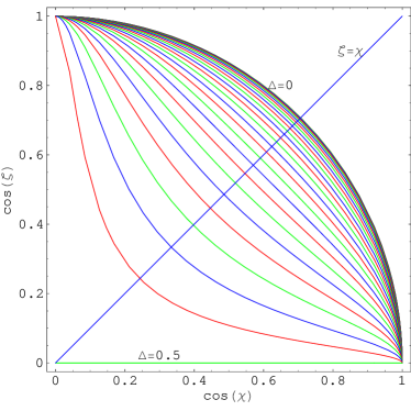
Figure 1: Peak separation $\Delta$ between both gamma-ray pulses purely determined by the obliquity of the pulsar $\chi$ and the inclination angle of the observer line of sight $\zeta$. Each curve represents a constant value of $\Delta$ ranging from 0 to 0.5 by 0.02 steps. No separation occurs along the circle of radius unity (pulse overlapping) whereas maximum separation of 0.5 is reached for $\cos\zeta=0$. The diagonal $\zeta=\chi$ describes the visibility of one magnetic pole.

The relation Eq. (24) was already noticed by Kirk (2005), see figure therein. For symmetry reasons, we will assume that $\chi\in[0,\pi/2]$, therefore $\cot\chi\geq 0$.

3.2 The radio lag $\delta$-peak separation $\Delta$ relation

Next, we show that the combination polar cap/striped wind allows to derive a simple analytical relation between the lag of radio vs gamma-ray arrival time $\delta$ and the high-energy peak separation $\Delta$. Because the two sites of emission are very distinct, inside and outside the light cylinder, the lag is interpreted as a time of flight delay between the region of radio radiation and the one for gamma-ray photon production.

The choice of origin of time and line of sight located in the plane $(Oyz)$ (therefore $\varphi=\frac{\pi}{2}$) implies that the radio photon emitted towards the observer will happen at periodic dates with period $P$, for one pole, given by

$$t_{\rm pc}^{\rm n}=\frac{\pi}{2\,\Omega_{*}}+k\,\frac{2\,\pi}{\Omega_{*}}=\frac{P}{4}+k\,P$$ (25)

where $k\in\mathbb{Z}$ is a natural integer. The superscript n denotes bundles of photons emanating from the same polar cap, let us say the north magnetic pole. The same applies to the south cap but due to the symmetry, the phase difference corresponds to half a period, $P/2$, thus

$$t_{\rm pc}^{\rm s}=t_{\rm pc}^{\rm n}+\frac{P}{2}=\frac{3\,P}{4}+k\,P$$ (26)

The observer remains at a distance $D$ from the center of the neutron star. The polar cap photon needs therefore a time $\Delta t=(D-R_{*})/c$ to reach him after emission from the pulsar. Thus the detection time is the sum

$$t_{1}=t_{\rm pc}^{\rm n}+\frac{D-R_{*}}{c}$$ (27)

The gamma-ray photon from the current sheets arrives earlier because closer to the observer, he needs a shorter flying time given by $\Delta t=(D-R_{0})/c$ leading to a time of detection given by

$$t_{2}=t_{\rm s}^{\pm}+\frac{D-R_{0}}{c}$$ (28)

As a consequence, the difference in arrival time between both kind of photons, focusing on the radio emission coming out of the north pole (visible for $0<\zeta<\pi/2$), is

$$t_{a} = t_{2}-t_{1}=t_{\rm s}^{\pm}-t_{\rm pc}^{\rm n}+\frac{R_{*}-R_{0}}{c}$$

$$= \frac{1-\beta_{\rm v}}{\beta_{\rm v}}\,\frac{R_{0}}{c}\pm\frac{\arccos(-\cot\zeta\,\cot\chi)}{\Omega_{*}}+\frac{R_{*}}{c}-(k+l)\,P$$

By normalizing this time to the period of the pulsar $P$ and using Eq. (22) with $\cot\zeta\,\cot\chi\geq 0$, we arrive at

$$\delta = \frac{t_{a}}{P}$$ (30)

$$= \frac{1-\beta_{\rm v}}{\beta_{\rm v}}\,\frac{R_{0}}{2\,\pi\,r_{\rm L}}\pm\frac{1-\Delta}{2}+\frac{R_{*}}{2\,\pi\,r_{\rm L}}-(k+l)$$ (31)

The same procedure applied to the south pole with $\pi/2<\zeta<\pi$ implies $\cot\zeta\,\cot\chi\leq 0$, leading to the same conclusion because of symmetry.

Recall that in order to observe pulsed emission from the radially expanding wind, the flow has to be relativistic with $\Gamma_{\rm v}\gg 1$ and $R_{0}$ must lie close enough to the light-cylinder such that the underlying condition is fulfilled

$$R_{0}\lesssim 2\,\pi\,\Gamma_{\rm v}^{2}\,r_{\rm L}$$ (32)

Thus the upper limit to the first term in Eq. (31) is

$$\frac{1-\beta_{\rm v}}{\beta_{\rm v}}\,\frac{R_{0}}{2\,\pi\,r_{\rm L}}\approx\frac{1}{2\,\Gamma_{\rm v}^{2}}\,\frac{R_{0}}{2\,\pi\,r_{\rm L}}\lesssim\frac{1}{2}$$ (33)

Moreover, for all the pulsars in the catalog, even for the millisecond pulsars, the light-cylinder radius is much larger than the stellar radius, $r_{\rm L}\gg R_{*}$. To a good approximation, we can neglect the term $\frac{R_{*}}{2\,\pi\,r_{\rm L}}$ in Eq. (31), the neutron star is located well within its light-cylinder. The remaining expression for a positive lag is

$$\delta\approx\frac{1-\Delta}{2}$$ (34)

This has to be compared with the $\delta-\Delta$ diagram published in Abdo et al. (2010a). The data points as well as the relation Eq. (34) are shown in Fig. 2. All the points but one lie below the line given by Eq. (34). The spread in radio lag along this line can be understood as a fluctuation in the precise location of the most significant emission in the wind.

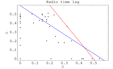
Figure 2: Gamma-ray peak separation $\Delta$ vs radio time lag $\delta$ as observed by Fermi-LAT. The blue curve is a linear fit and the red straight line the upper limit as predicted by Eq. (34).

Finally, we give an expression for the linear fit to the sample of pulsars showing double peaked gamma-ray light-curves simultaneously with radio emission by

$$\Delta_{\rm fit}\approx 0.59-1.06\,\delta$$ (35)

shown in blue line in Fig. 2.

3.3 Other retardation effects

Including general-relativistic effects do not change much the time lag between radio and gamma-ray photons. Indeed using the Schwarzschild geometry, for a photon with radial motion, the time required to reach a distant observer located at a distance $D$, starting on the stellar surface is

$$c\,\Delta t_{\rm pc}=D-R_{*}+R_{s}\,\ln\left(\frac{D-R_{s}}{R_{*}-R_{s}}\right)$$ (36)

$R_{s}=2\,G\,M/c^{2}$ being the Schwarzschild radius. A similar expression applies for gamma-rays

$$c\,\Delta t_{\gamma}=D-R_{0}+R_{s}\,\ln\left(\frac{D-R_{s}}{R_{0}-R_{s}}\right)$$ (37)

Therefore the time of flight difference compared to Newtonian gravity is

$$\Delta t_{\rm GR}=\Delta t_{\gamma}-\Delta t_{\rm pc}=\frac{R_{*}-R_{0}}{c}+\frac{R_{s}}{c}\,\ln\left(\frac{R_{*}-R_{s}}{R_{0}-R_{s}}\right)$$ (38)

Normalized to the pulsar period we get an increase by an amount of

$$\delta_{\rm GR}=\frac{R_{s}}{2\,\pi\,r_{\rm L}}\,\ln\left(\frac{R_{*}-R_{s}}{R_{0}-R_{s}}\right)$$ (39)

For neutron star parameters, this remains negligible compared to unity because $R_{s}\ll r_{\rm L}$. Typical values are $\delta_{\rm GR}\approx 0.01$.

3.4 Phase-inclination diagram

Next, we show the phase-inclination diagram for different inclinations of the line of sight $\zeta$ as well as different magnetic obliquities $\chi$ of the pulsar. This is done for the high-energy photons as well as for the radio emission coming from the polar cap, see Fig. 3. In order to point out the relative phase shift between both emission processes, we normalized independently their respective maximum intensity to unity. The continuous rotated S-shaped structure is a characteristic of the striped wind whereas the two spots correspond to a mapping of the two polar caps. Both structures are symmetric with respect to the equatorial plane, i.e. compared to an inclination $\zeta=90^{o}$, as expected from the geometry.

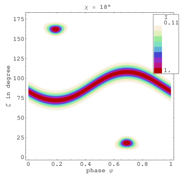
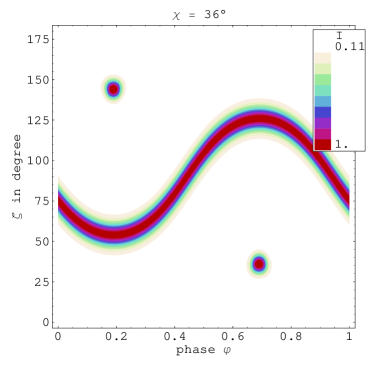
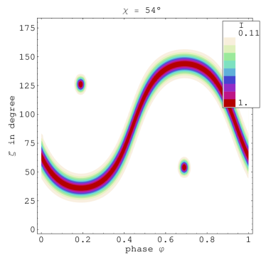
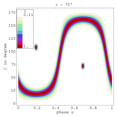
Figure 3: Phase plot of the pulsed gamma-ray and radio emission components for a full period of the pulsar (phase $\in[0,1]$) for an inclination of the line of sight $\zeta$ between 0 and 180 degrees and magnetic obliquities $\chi=18,36,54$ and $72$ degrees, from top left to bottom right. Note the colour-coded range shown in the legends of each phase plot: white colour corresponds to the faintest phase (off pulse) with intensity around 0.11 whereas red colour corresponds to the brightest luminosity i.e. 1 (in normalized unities).

The observer will see different kind of light-curves depending on his viewing angle. First, radio photons are observable only when the line of sight intersects at least one polar cap, in the vicinity of the magnetic poles, that is when $\zeta\approx\chi\pm\vartheta_{\rm pc}$. Second, to observe the gamma-ray pulsation, this same line of sight should intersect the current sheets, or in other words $\pi/2-\chi\leq\zeta\leq\pi/2+\chi$. Conversely, no gamma-ray pulses are seen when $\zeta\leq\pi/2-\chi$ or $\zeta\geq\pi/2+\chi$. Thus a necessary condition to detect simultaneously radio and gamma-ray photons is $\chi\geq\pi/4$ and $\zeta\approx\chi$. For those particular pulsars, possessing a double gamma-ray peak and radio emission, we are able to find the geometrical parameters from the peak separation, see Fig. 1. Third, a single pulse in the high-energy light-curve occurs when the line of sight passes just through the edge of the striped part of the wind, this can be interpreted as the special case $\zeta\approx\pi/2-\chi$. In the very special case of one gamma-ray pulse and observable radio emission, this leads immediately to the geometrical parameters $\zeta\approx\chi\approx\pi/4=45^{o}$. This seems to be the case for PSRJ0437-4715 and PSRJ2229+6114.

The phase plots shown in Fig. 3 have been computed for different inclination angles $\zeta$ and obliquities $\chi$ but with constant current sheet thickness, parameterized by $\Delta_{\varphi}$, and constant particle density contrast, which means constant ratio $N/N_{0}$. More precisely, we adopted $\Delta_{\varphi}=10$ and $N/N_{0}=10$. This last value explain the factor around 10 in intensity between off-pulse and on-pulse phase. Indeed, by decreasing the fluctuation in particle density between the hot unmagnetized and cold magnetized part of the wind, as done in Fig. 4, we recognize a similar trend in the intensity diagram. If the ratio $N/N_{0}=5$, the luminosity varies between $0.22\approx 1/5$ and $1$ in normalized unities whereas for $N/N_{0}=2$, it lies between $0.54\approx 1/2$ and 1.

Moreover, the current sheet thickness directly impacts on the duty cycle of the light-curve, or in other words, on the width of the gamma-ray pulses. This has been check by changing the parameter $\Delta_{\varphi}$ to 5 or 2 instead of the previous value of 10. Results are shown in Fig. 5.

To better assess the differences, we summarize all the light-curves for $\chi=72$ degrees and $\zeta=90$ degrees in two plots as depicted in Fig.6.

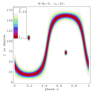
Figure 4: Phase plot of the pulsed gamma-ray and radio emission components for a full period of the pulsar (phase $\in[0,1]$) for an inclination of the line of sight $\zeta$ between 0 and 180 degrees and a magnetic obliquity $\chi=72$ degrees. Only the ratio $N/N_{0}$ changes.

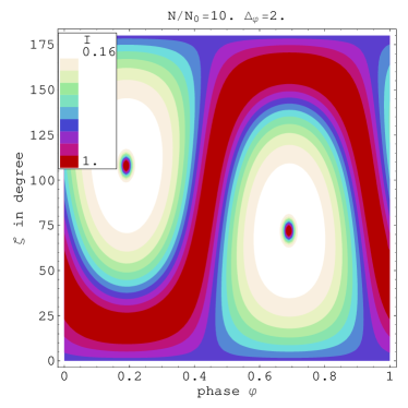
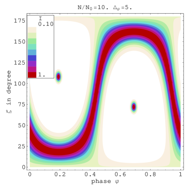
Figure 5: Phase plot of the pulsed gamma-ray and radio emission components for a full period of the pulsar (phase $\in[0,1]$) for an inclination of the line of sight $\zeta$ between 0 and 180 degrees and a magnetic obliquity $\chi=72$ degrees. Only the parameter $\Delta_{\varphi}$ varies.

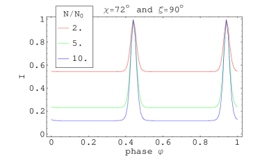
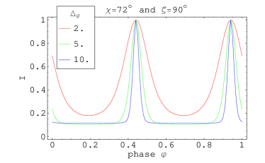
Figure 6: Light-curves of the pulsed gamma-ray emission component, for a full period of the pulsar (phase $\in[0,1]$) and for an inclination of the line of sight $\zeta=90$ degrees and a magnetic obliquity $\chi=72$ degrees. On the left picture, for different parameters $N/N_{0}$ with $\Delta_{\varphi}=10$ and on the right picture for different $\Delta_{\varphi}$ with $N/N_{0}=10$.

Finally, there exist two limiting cases. First the aligned rotator showing no pulsed emission. Second the perpendicular rotator emits pulsed high-energy radiation over the whole sky and both its polar caps are visible. A direct consequence is a double peak structure in both radio and gamma-ray light-curves, with a separation of $\Delta=0.5$. PSRJ0030+0451 is a typical example.

3.5 Flux correction factor

The photon flux $F_{\rm obs}$ measured by an observer located on Earth is biased due to anisotropic emission from the wind depending on the viewing angle $\zeta$. This fact is clear from the aforementioned phase-inclination plots shown in the previous paragraphs. The observed gamma-ray flux has to be corrected to obtain the true gamma-ray luminosity by introducing a correction factor $f_{\Omega}$ defined by

$$L_{\gamma}=4\,\pi\,f_{\Omega}\,F_{\rm obs}\,D^{2}$$ (40)

Here $D$ is the distance of the pulsar to the observer and $F_{\rm obs}$ the observed flux. As in the polar cap and outer/slot gap models (Watters et al., 2009), the correction implied here by a relativistic beaming effect is given by

$$f_{\Omega}(\chi,\zeta_{E})=\frac{\int_{0}^{\pi}\int_{0}^{2\,\pi}F_{\gamma}(\chi,\zeta,\varphi)\,\sin\zeta\,d\zeta\,d\varphi}{2\,\int_{0}^{2\,\pi}F_{\gamma}(\chi,\zeta_{E},\varphi)\,d\varphi}$$ (41)

For the striped wind model, this correction factor is shown in fig. 7 with the full dependence on obliquity $\chi$ and inclination of Earth line of sight $\zeta_{E}$.

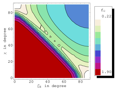
Figure 7: Flux correction factor $f_{\Omega}$ for the striped wind model vs obliquity $\chi$ and inclination of Earth line of sight $\zeta_{E}$. Two different regions with roughly constant factor are clearly distinguishable along $\zeta_{E}=\pi/2-\chi$.

We can approximately separate the correction factor into two regions of constant value. In the first region, for an obliquity $\chi<\pi/2-\zeta_{E}$, the correction is close to be uniform and equal roughly to 1.90. This case corresponds to a line of sight not crossing the current sheets in the wind, there is almost no pulsed emission visible. In the second region, where $\chi>\pi/2-\zeta_{E}$, the correction is also almost uniform and equal roughly to 0.4. This case corresponds to a line of sight intersecting the current sheets, leading to pulsed emission. This behavior is expected from the definition of the correction factor Eq. (41). Indeed, for a fixed obliquity $\chi$, the numerator is a constant whereas the denominator depends on the line of sight towards the Earth. On one side, in the first region $\chi>\pi/2-\zeta_{E}$, the phase-averaged emission is faint and weakly pulsed. It follows a small denominator therefore a large correction factor. On the other side, in the second region, the situation is opposite, the emission during the pulses is strong and so the denominator of Eq. (41) larger, finally the correction factor is weakest.

Note that these bounding values depend on the sheet thickness parameterized by $\Delta_{\varphi}$ as well as on the particle density contrast parameterized by $N_{0}$ and $N$.

3.6 Light-curve fitting and gamma-ray luminosity

We conclude our study by fitting light-curves of a small sample of pulsars. The only relevant free parameters in our model are the geometry of the wind, the particle density number and the size of the current sheets. In this last section, we specialize our results to some Fermi detected gamma-ray pulsars and show the best parameters fitting their high-energy light-curves above 100 MeV. Therefore, the knowledge of the viewing angle and the obliquity allows an estimation of the flux correction via the beaming factor. Eventually a true gamma-ray luminosity versus spin-down luminosity can be plotted.

We start with an estimate of the peak separation when one radio pulse is detected. In that case, $\zeta\approx\chi$ as explained above and the knowledge of $\Delta$ immediately implies a solution for $\zeta$. This has been done for several pulsars and listed in Tab. 1. In all the results shown below, for simplicity, we took a constant Lorentz factor of the wind equal to $\Gamma_{\rm v}=10$.

Pulsar	$\delta$ (obs)	$\Delta$ (obs)	$\chi$	$\zeta$	$\delta$ (model)	$\Delta_{\varphi}$	$N/N_{0}$	$f_{\Omega}$	$L_{\gamma}$	$L_{\gamma}$ (corrected)	efficiency $\eta$
			deg	deg	$(1-\Delta)/2$				$10^{26}$ W	$10^{26}$ W
J0030+0451	0.18	0.44	67	85	0.28	5	10	1.17	0.57	0.49	0.16
J0218+4232	0.32	0.36	57	75	0.32	3	3	1.10	27-69	24-62	0.10-0.26
J0437-4715	0.43	-	45	40	0.5	10	10	1.07	0.054	0.050	0.016
J1124-5916	0.23	0.49	80	85	0.255	5	3	1.20	100	83	0.007
J2021+3651	0.17	0.47	73	65	0.265	10	10	1.14	250	220	0.065
J2032+4127	0.15	0.50	89	70	0.25	5	3	1.18	34-170	29-145	0.11-0.55
J2043+2740	0.20	0.36	57	65	0.32	5	3	1.05	6	5.7	0.10
J2229+6114	0.49	-	45	40	0.5	10	10	1.07	17-1100	16-1026	0.0007-0.045

Table 1: Geometry of the pulsar wind for 8 gamma-ray pulsars. The angle of inclination and obliquity are given in degrees. The Lorentz factor of the wind is the same for the whole sample and taken to be $\Gamma_{\rm v}=10$.

Let us have a deeper look on a representative sample of Fermi-detected gamma-ray pulsars.

3.6.1 PSR J0030+0451

PSR J0030+0451 is a millisecond pulsar, $P=4.87$ ms, showing a double pulse structure in the radio band. This may suggest that both its magnetic poles are visible, or in other words, it is almost a perpendicular rotator with $\chi\approx 90^{o}$. Nevertheless, the maximal intensity of both radio pulses are sensibly different, this is interpreted as the line of sight passing closer to one magnetic pole than to the other. An alternative would be to explain it by a process occurring in the vicinity of the polar caps with variable efficiency. However, polar cap emission is not the main purpose of this work so we simply assume identical shapes for both radio-pulses. Therefore, an obliquity close to $90$ degrees but less matches the right geometry. Setting $\chi\approx 67^{o}$ satisfactorily agrees with the radio light-curve, see Fig. 8, on the top left plot. To have the right gamma-ray peak separation, we have to adopt $\zeta\approx 85^{o}$. Moreover, the radio-pulses are very broad, each of them having a duty cycle of roughly $0.2$ in phase. Therefore, to reconcile our model with data, we have to extend the polar cap region to a sizeable fraction of the whole neutron star surface, Fig. 8, top left plot. Emission starts right after the light-cylinder radius. There is still a excess of 0.1 in the phase delay compared to observation. This has to be explained by some other retardation effects of the radio pulse such as the strong gravitational field regime (which we have shown to be negligible) or by magnetic field bending due to charges flowing within the magnetosphere and disturbing the closed field lines structure taking to be an exact dipole.

3.6.2 PSR J0218+4232

PSR J0218+4232 is another millisecond pulsar, $P=2.32$ ms, showing a less clear double pulse structure in gamma-rays. Its radio-pulse shape looks much more complicated with something like conal and core component, over a wide range of the pulsar period. The best fit is obtain for an obliquity $\chi=57^{o}$ and an inclination of $\zeta=75^{o}$. The gamma-ray light curve adjusts well to Fermi data. Moreover the gamma-ray pulse time lag compared to the middle of the radio pulse matches precisely the measurements. Note that the gamma-ray off pulse emission remains at an appreciable level over the full period, see Fig. 8, on the top right plot.

3.6.3 PSR J0437-4715

PSR J0437-4715 is a special case of millisecond pulsar, $P=5.76$ ms, showing only one gamma-ray pulse combined with a sharp radio pulse. As explained in a previous discussion, the unique geometry allowing such a behavior needs an obliquity almost equal to the inclination of the line of sight, namely $\zeta\approx\chi\approx 45^{o}$. Indeed, we take $\chi=45^{o}$ and $\zeta=40^{o}$ and arrive at the light curve presented in Fig. 8, second row, left plot. For one gamma-ray pulse, our model predicts a delay of $0.5$ in phase between radio and gamma-ray pulsars, in relative good agreement with Fermi measuring $0.43$. The overestimate is about 0.07.

3.6.4 PSR J1124-5916

PSR J1124-5916 shows a sharp double gamma-ray peak with significant off-pulse emission in combination with a single radio peak. Adopting the parameters $\chi=80^{o}$ and $\zeta=85^{o}$, our model is compared with observation in Fig. 8, second row, right plot. The expected time lag $0.255$ is not very different from the measured $0.23$.

3.6.5 PSR J2021+3651

PSR J2021+3651 gamma-ray light-curve shows a narrow double pulse structure and a single radio pulse. The peak separation is close to $0.5$. Here again, for the best fit parameters $\chi=73^{o}$ and $\zeta=65^{o}$, the predicted lag of $0.265$ overshoots the observation by roughly $0.1$, Fig. 8, third row, left plot.

3.6.6 PSR J2032+4127

PSR J2032+4127 is an example of half-a-period peak separation implying a line of sight inclination of $\zeta\lesssim 90^{o}$. Moreover, because we see radio pulse it should be almost a perpendicular rotator. However, this would permit to detect both radio component which is not the case, so we must conclude that the inclination is slightly different from an orthogonal rotator with a small polar cap reproducing a width of 0.1 in the radio pulse, Fig. 8, third row, right plot. We found best agreement for $\chi=89^{o}$ and $\zeta=70^{o}$.

3.6.7 PSR J2043+2740

It seems that PSR J2043+2740 shows evidence for three gamma ray pulses, Fig. 8, bottom left plot. The two extreme ones are significant whereas the middle one is less significant. We tried to fit the light curve according to the two well separated pulses. The time delay is overestimated by $0.12$.

3.6.8 PSR J2229+6114

Finally, PSR J2229+6114 is another example of single pulse gamma-ray pulsar. The best fit parameters correspond to the same values as for PSR J0437-4715. Now, the time lag is even better, again the model predicts $0.5$ compared to the observed $0.49$, Fig. 8, bottom right plot.

Details of the parameters used to fit the data are summarized in Tab. 1.

This ends the sample of fitted gamma-ray pulsars. We demonstrated that our striped wind/polar cap model implies a well-defined relation between gamma-rays and radio pulses. Single and double pulse light-curves are expected. For some pulsars, the model does well in explaining this relationship. However, it seems that some others pulsars possess time lag slightly less than the expected value, on average it is smaller by an amount of $0.1$ in phase. This has probably to find its root in the geometry of the polar cap or in retardation effects not taking into account in this investigation.

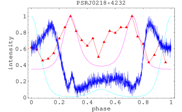
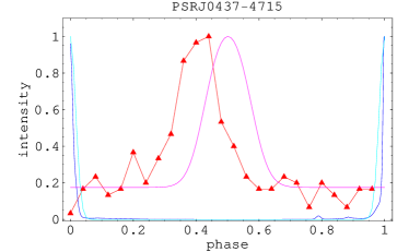
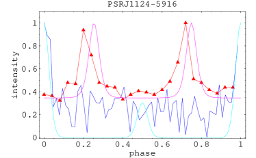
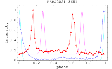
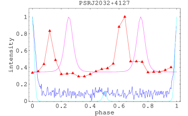
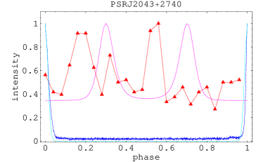
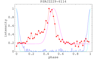
Figure 8: Gamma-ray (red lines) and radio (blue lines) light-curves of several pulsars fitted with the combined polar cap/striped wind model. Intensities are normalized to unity.

3.6.9 Corrected gamma-ray luminosity

Finally, knowing the precise geometry from the light-curves and time lag, we computed the flux correction factor for each of the above mentioned pulsar and summarize our results in Tab.1. The “true” efficiency is also given therein.

4 CONCLUSION

By combining the striped wind model with a simple prescription for the polar cap geometry and emission, we were able to derive the time lag between radio and gamma rays according to the high-energy pulse separation, if available, in agreement with recent Fermi observations from the first gamma-ray pulsar catalog. According to our composite model, it seems that the observed gamma-ray pulsation is generated just outside the light-cylinder and radio pulses come from low altitude polar cap locations.

A further careful inspection of individual pulsar light-curves, the correlation between their radio and gamma-ray peaks, will permit to severely constrain the geometry, deducing the obliquity and inclination of line of sight of the system.

The overestimate of time lag by roughly 0.1 in phase for many pulsars suggest that another ingredient is still missing to fit properly the data. As shown, curved space-time is negligible, so we expect magnetic field line bending and/or plasma flow within the magnetosphere and other plasma effects to give us some clue to this enigma.

References

- Abdo et al. (2010a) Abdo, A. A., Ackermann, M., Ajello, M., et al. 2010a, ApJS, 187, 460
- Abdo et al. (2010b) Abdo, A. A., Ackermann, M., Ajello, M., et al. 2010b, ApJ, 708, 1254
- Abdo et al. (2010c) Abdo, A. A., Ackermann, M., Ajello, M., et al. 2010c, ApJ, 720, 272
- Abdo et al. (2009) Abdo, A. A., Ackermann, M., Atwood, W. B., et al. 2009, ApJ, 696, 1084
- Bai & Spitkovsky (2010a) Bai, X. & Spitkovsky, A. 2010a, ApJ, 715, 1282
- Bai & Spitkovsky (2010b) Bai, X. & Spitkovsky, A. 2010b, ApJ, 715, 1270
- Bogovalov (1999) Bogovalov, S. V. 1999, A&A, 349, 1017
- Cheng et al. (1986) Cheng, K. S., Ho, C., & Ruderman, M. 1986, ApJ, 300, 500
- Coroniti (1990) Coroniti, F. V. 1990, ApJ, 349, 538
- Dyks et al. (2004) Dyks, J., Harding, A. K., & Rudak, B. 2004, ApJ, 606, 1125
- Kirk (1994) Kirk, J. G. 1994, in Saas-Fee Advanced Course 24: Plasma Astrophysics, ed. A. O. Benz & T. J.-L. Courvoisier, 225–+
- Kirk (2005) Kirk, J. G. 2005, Memorie della Societa Astronomica Italiana, 76, 494
- Kirk et al. (2009) Kirk, J. G., Lyubarsky, Y., & Petri, J. 2009, in Astrophysics and Space Science Library, Vol. 357, Astrophysics and Space Science Library, ed. W. Becker, 421–+
- Kirk et al. (2002) Kirk, J. G., Skjæraasen, O., & Gallant, Y. A. 2002, A&A, 388, L29
- Michel (1994) Michel, F. C. 1994, ApJ, 431, 397
- Pétri (2009) Pétri, J. 2009, A&A, 503, 13
- Pétri & Kirk (2005) Pétri, J. & Kirk, J. G. 2005, ApJL, 627, L37
- Pétri & Kirk (2007) Pétri, J. & Kirk, J. G. 2007, Plasma Physics and Controlled Fusion, 49, 1885
- Radhakrishnan & Cooke (1969) Radhakrishnan, V. & Cooke, D. J. 1969, Astrophysical Letters, 3, 225
- Romani & Watters (2010) Romani, R. W. & Watters, K. P. 2010, ApJ, 714, 810
- Venter et al. (2009) Venter, C., Harding, A. K., & Guillemot, L. 2009, ApJ, 707, 800
- Watters et al. (2009) Watters, K. P., Romani, R. W., Weltevrede, P., & Johnston, S. 2009, ApJ, 695, 1289