What makes slow samples slow in the Sherrington-Kirkpatrick model

Abstract

Using results of a Monte Carlo simulation of the Sherrington-Kirkpatrick model, we try to characterise the slow disorder samples, namely we analyse visually the correlation between the relaxation time for a given disorder sample $J$ with several observables of the system for the same disorder sample. For temperatures below $T_{c}$ but not too low, fast samples (small relaxation times) are clearly correlated with a small value of the largest eigenvalue of the coupling matrix, a large value of the site averaged local field probability distribution at the origin, or a small value of the squared overlap $<q^{2}>$. Within our limited data, the correlation remains as the system size increases but becomes less clear as the temperature is decreased (the correlation with $<q^{2}>$ is more robust) . There is a strong correlation between the values of the relaxation time for two distinct values of the temperature, but this correlation decreases as the system size is increased. This may indicate the onset of temperature chaos.

The Sherrington-Kirkpatrick (SK) model has been intensively studied since the mid-seventies, when it was introduced [1] as a starting point for studying spin glasses. It has a low temperature spin glass phase, with a very slow dynamics and an equilibrium relaxation time that diverges when the number of sites $N$ goes to infinity. The value of the equilibrium relaxation time $\tau$ depends strongly on the disorder sample $J$, and $\tau$ is not self averaging (namely $\Bigl{[}E(\tau^{2})-E(\tau)^{2}\Bigr{]}/E(\tau)^{2}$, where $E(\cdot)$ is the disorder average, does not go to zero as $N\to\infty$). There are now reasonable evidences, both analytical and numerical (see [2, 3] and references therein) that, in the low temperature phase of the model, the disorder average of the logarithm of the equilibrium relaxation time $E(\ln{\tau})$ grows like $N^{1/3}$ as $N$ grows, and that the probability density function of $\ln{\tau}$ scales according to the equation $P(\ln{\tau})=N^{-\psi}F((\ln{\tau}-E(\ln{\tau}))/N^{\psi})$, with some $N$ independent function $F(\cdot)$ with zero mean, and $\psi=1/3$, although it has been argued[4, 5] that $\psi$ may be slightly less than $1/3$ (In such a case $\ln{\tau}$ would be weakly self averaging).

Whether $\psi$ is equal to $1/3$ or slightly less than $1/3$, there are definitively disorder samples with extremely slow dynamics. Our aim in this note is to try to characterise these “slow samples”. We have two motivations in mind, one theoretical and the other more down to earth. The first motivation is the question of the behaviour of $F(x)$ for large values of the argument $x$. It has been argued in [4] that $F(x)$ has an exponential behaviour with $\ln F(x)\propto-x^{\eta}$ for large $x$. If furthermore the tail of $F(x)$ is dominated by rare disorder samples with small probability $\propto\exp(-AN^{\alpha})$ and an anomalously large free energy barrier $\propto N^{\beta}$ (with $\beta>1/3$), the exponents $\alpha$, $\beta$, $\psi$ and $\eta$ fulfil [4] the consistency relation $(\beta-\psi)\eta=\alpha$. For example, a dominance by the rare samples with all exchange couplings $J_{i,j}$ positive (up to a gauge transformation, see later) would correspond to $\alpha=2$, and $\beta=3/2$. The value $\psi=1/3$ would then imply that $\eta=12/7$. This value for $\eta$ is however not compatible with the numerical results of [4] for the distribution $P(\log{\tau})$. In this reference arguments are given for the values $\alpha=\beta=1$, $\psi=1/4$ (and accordingly $\eta=4/3$) instead. The second motivation for the characterisation of the slow samples is of practical matter for Monte Carlo simulations: The vast majority of the Monte Carlo simulations of disordered systems in the literature use the same number of iterations for all disorder samples . There is accordingly a danger that some rare slow disorder samples are not thermalized. One is led naturally to the idea of concentrating the computational effort on the hard samples, that may require orders of magnitude more iterations than the mainstream disorder samples. Since the measurement of the relaxation time for every disorder sample is very time consuming, any heuristic method to pinpoint the slow samples can be valuable.

The numerical method used is similar to the one used in [3]. We consider the SK model with binary exchange couplings, and the Hamiltonian

$${\cal H}=-\frac{1}{2}\sum_{i\neq j}J_{i,j}\sigma_{i}\sigma_{j}\ ,$$ (1)

with $\sigma_{i}=\pm 1$, $J_{i,j}=\pm 1/\sqrt{N}$. We measure the dynamic overlap

$$q_{d}(t)=\frac{1}{N}\sum_{i=1}^{N}\sigma_{i}(t_{0})\sigma_{i}(t+t_{0})\ ,$$ (2)

averaged along a very long trajectory (namely averaging over many values of $t_{0}$), with the Metropolis dynamics, starting from a well equilibrated spin configuration (obtained with the parallel tempering algorithm). Obviously $q_{d}(0)=1$ and $q_{d}(t)$ decreases continuously towards zero, as $t$ grows. We define the relaxation time $\tau$ by the equation $q_{d}(t=\tau)=1/2\sqrt{E(<q^{2}>)}$, where $q$ is the usual ($J$ dependent) overlap between two replica. Here we depart from [3] where a definition involving $<q^{2}>$, with no disorder average, was used. Indeed, since we are looking for correlations between the value of $\ln{\tau}$ and other $J$ dependent quantities (including $<q^{2}>$ itself), it seems more appropriate to define $\tau$ using a sample independent condition. The parameters of the simulations are such that our estimates of $\ln{\tau}$ have negligible thermal noise, as compared to the disorder sample to disorder sample fluctuations (see [3] for details). That the thermal noise is tamed is an essential condition for our analysis. We have data for $N=64$ to $512$, $1024$ disorder samples, and temperatures $T=0.4,0.5,\ldots$ (The critical temperature is $T_{c}=1$).

Note that as in [3] we do not measure relaxation times larger than some $t_{window}\approx 3.7\ 10^{6}$ (and $t_{window}\approx 1.7\ 10^{6}$ for $N=512$.). For a given couple $N$ and $T$, the disorder samples with relaxation time larger than $t_{window}$ are thus “censored”. By convention, $\ln{\tau}=-1$ for such samples, namely minus one means overflow. Note that the real $\ln{\tau}$ is never equal to minus one (our relaxation times are integers).

As explained just before, we found it more proper to define the relaxation time using a condition involving the disorder averaged $E(<q^{2}>)$ rather than $<q^{2}>$ as was done in [3]. It turns out however that this makes little difference as shown in figure 1 where we compare the two definitions in the case $N=128$, $T=0.4$. The same conclusion holds for other couples of $N$ and $T$. On close look, one notices that for low values of $\ln{\tau}$ the definition used here gives systematically lower results than the one used in [3]. This is explained by the fact that low values of $\ln{\tau}$ are strongly correlated to low values of $<q^{2}>$ (see later in the text and figure 5). This small systematic difference between the two definitions of the relaxation time disappears when $\ln{\tau}$ grows.

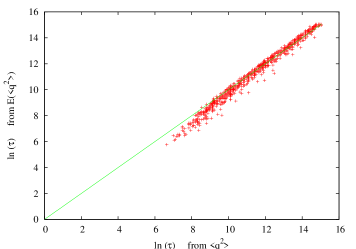
Figure 1: Plot of $\ln{\tau}$, as measured using the definition of this note, as a function of the value obtained using the definition used in [3]. Here $N=128$ and $T=0.4$. The straight line is the diagonal. There are no disorder samples with $\tau>t_{window}$ in the data.

The first question we would like to address is whether the tail of the distribution $P(\ln{\tau})$ is dominated by ferromagnetic disorder configurations. In order to proceed, we need a measure of the ferromagnetic character of a disorder configuration. The sum $\sum_{i\neq j}J_{i,j}$ is not a suitable indicator since it is not invariant under the local gauge symmetry of the model $\sigma_{i}\to\epsilon_{i}\sigma_{i}$, $J_{i,j}\to\epsilon_{i}\epsilon_{i}J_{i,j}$ with $\epsilon_{i}=\pm 1$, whereas the dynamics is invariant under this symmetry. Said another way, for every disorder configuration with all $J_{i,j}>0$, there is a huge number of $2^{N}-1$ other gauge transformed configurations with the same value of $\ln{\tau}$ (and the same weight) but a different value of $\sum_{i\neq j}J_{i,j}$, and any correlation is washed out. (We nevertheless checked that there is indeed no sign of correlations between $\ln{\tau}$ and $\sum_{i\neq j}J_{i,j}$ in our data). A better indicator of the ferromagnetic character of a disorder configuration, that has been proposed in [5], is the largest eigenvalue $\lambda_{N}$ of the matrix $\{J_{i,j}\}$. In the SK model the diagonal elements of this matrix are not used, but they are obviously needed however in order to compute the eigenvalues of the matrix, and we have set them equal to zero. Our results for the correlation between $\ln{\tau}$ and $\lambda_{N}$ can be found in figure 2 for $N=64$ and $T=0.8$. The points on the $x$ axis are concentrated around the value two, in agreement with random matrix results for the GOE with the normalisation $E(J_{i,i}^{2})=1/N$ for $i\neq j$ (in the GOE the diagonal elements are random with $E(J_{i,i}^{2})=2/N$, and not identically zero, but this should not change the asymptotic behaviour). There is a clear correlation between low values of $\lambda_{N}$ and low values for $\ln{\tau}$, but this correlation becomes fuzzy as $\lambda_{N}$ grows. We were looking for a characterisation of the slow disorder samples but we found a characterisation of the fast disorder samples instead.

The scatter plots become progressively harder to interpret as $N$ grows and / or $T$ decreases, since we are missing more and more points that correspond to censored values of $\ln{\tau}$. One can nevertheless conclude from our data that the correlation remains as the system size increases, but becomes more fuzzy as temperature is decreased. (The neat correlation seen in the left of figure 2 fades away as the temperature is decreased). The net conclusion is that there is in our data no visible dominance of the large relaxation region by ferromagnetic disorder samples . This is in agreement with the findings of [4] for the tail of the distribution of $\ln{\tau}$.

In the spherical SK model [8] the relaxation time is fixed by the difference between the two largest eigenvalues of the $\{J_{i,j}\}$ matrix, through the equation

$$\ln{\tau}=N/(2T)(1-T)(\lambda_{N}-\lambda_{N-1})\ .$$ (3)

For the SK model with binary couplings we consider here, the correlation between $\ln{\tau}$ and $\lambda_{N}-\lambda_{N-1}$ is more fuzzy, as one can see in figure 3. It is in fact fuzzier than the relation between $\ln{\tau}$ and $\lambda_{N}$ alone. This is true for all values of $N$ and $T$ considered, and for all values of $\ln{\tau}$ (both large and small). Note that in the spherical SK model, equation 3 is used to prove that $E(\ln{\tau})\propto N^{1/3}$. It turns out [2] that this scaling holds also in the usual SK model although equation 3 does not hold.

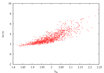
Figure 2: The logarithm of the relaxation time as a function of the largest eigenvalue $\lambda_{N}$ of the $\{J_{i,j}\}$ matrix for $N=64$ and $T=0.8$. There are no disorder samples with $\tau>t_{window}$ in the data.

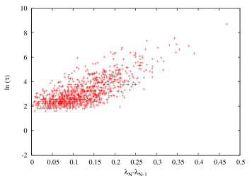
Figure 3: The logarithm of the relaxation time as a function of the gap between the two largest eigenvalues of the $\{J_{i,j}\}$ matrix for $N=64$ and $T=0.8$. There are no disorder samples with $\tau>t_{window}$ in the data.

In the spirit of [4], we have also looked at the correlation between $\ln{\tau}$ and the site averaged local field probability distribution $P(h_{local})$

$$P(h_{local})=\frac{1}{N}(<\sum_{i}\delta(h-\sum_{j\neq i}\ J_{i,j}\sigma_{j})>)\ .$$ (4)

Specifically we looked at the correlation between $\ln{\tau}$ and the value of $P_{(}h_{local})$ at the origin. Our results can be found in figure 4 for $N=64$ and $T=0.8$. In [4] it was argued that the disorder samples with large relaxation times are the ones with all local fields (on every site $i$) large. This is indicative of a correlation between large values of $\ln{\tau}$ and a distribution $P_{(}h_{local})$ that is depleted at the origin. (Indeed [10] $\ln{\tau}$ increases as $T$ decreases, while $P(h_{local}=0)$ decreases as $T$ decreases, with $P(h_{local}=0)=0$ at zero temperature in the $N=\infty$ limit). Our data indeed show a neat correlation between large values of $P(h_{local}=0)$, and small $\ln{\tau}$, but this correlation becomes fuzzy for lower values of $P(h_{local}=0)$. Again we were looking for a characterisation of the slow disorder samples but we found a characterisation of the fast disorder samples instead. The observed correlation seems to persists as $N$ grows, but fades as $T$ is decreased. There is a similar correlation between $\ln{\tau}$ and the average value of $h_{local}$ within the tail of $P(h_{local})$, for example within the last five percents of the distribution. A small value of $h_{local}$ inside the tail is correlated to a small relaxation time.

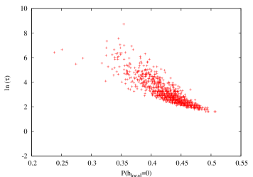
Figure 4: The logarithm of the relaxation time as a function of $P(h_{local}=0)$ for $N=64$ and $T=0.8$. The normalisation is such that $\int_{0}^{\infty}dh_{local}P(h_{local})=1$. There are no disorder samples with $\tau>t_{window}$ in the data.

The strongest correlation we found is between $\ln{\tau}$ and the average overlap squared $<q^{2}>$, as can be seen in figure 5. The observed correlation seems to persists as $N$ grows, and as $T$ is decreased. This correlation is an empirical finding and we have no dynamical explanation for it. On the other hand $<q^{2}>$ is fairly easy to estimate with Monte Carlo, even with little statistics and this correlation could be used to flag slow samples in numerical simulations. We finally remark that if there is a correlation between $\ln{\tau}$ and the average overlap squared $<q^{2}>$, there is no correlation between $\ln{\tau}$ and the number of peaks in the order parameter distribution $P(q)$. We have looked for such a correlation using the data of [9], where the number of peaks was estimated for a subset of the disorder samples considered here. The presence of thermal noise in the measured distribution makes it difficult to count the number of peaks. In this reference the authors did their best to count the number of peaks by visual inspection of the plots of $P(q)$ for $192$ disorder samples, with $T=0.4$. We find no correlation between the value of $\ln{\tau}$ and the number of peaks for $N=64$ and $256$.

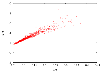
Figure 5: The logarithm of the relaxation time as a function of $<q^{2}>$ for $N=64$ and $T=0.8$. There are no disorder samples with $\tau>t_{window}$ in the data.

We have found finally that, disorder sample by disorder sample, the relaxation time measured at two temperatures (both in the spin glass phase) are strongly correlated. This can be seen in figure 6 where we show $\ln{\tau(T=0.5)}$ as a function of $\ln{\tau(T=0.6)}$ both for $N=64$. This figure shows a very strong correlation. One notice a couple of samples for which $\ln{\tau}(T=0.5)=-1$ (censored data). Figure 7 shows the same figure but with all systems sizes together. Obviously there are more and more disorder samples censored as $N$ grows, with now a whole horizontal segment with $\ln{\tau}=-1$. Interestingly all points in the scatter plot scale on the same $N$ independent thick line. This thick line would extend further towards large values had we used a larger observation window. (But it would be quite CPU time consuming to obtain a large extension). Note that the $N=512$ data appear to be more scattered than the other data, an optimistic interpretation is that we are seeing some onset of a temperature chaotic behaviour. In order to be more quantitative, we have analysed the data as follows: first we made a linear least squares fit of the $N=64$ data to the form $\ln{\tau}(T=0.5)=a+b\ln{\tau}(T=0.6)$, with parameters $a$ and $b$ (we obtain the values $a=0.195$ and $b=1.297$). Then we computed, for every system size $N$, the deviation $\delta_{N}^{2}=1/(N_{J}(1+b^{2}))\sum_{J}\bigl{(}a+b\ln{\tau}(T=0.6)-\ln{\tau}(T=0.5)\bigr{)}^{2}$, with the values of $a$ and $b$ obtained from the fit of the $N=64$ data, an a sum over those disorder samples such that both relaxation times are less than $t_{window}(N/512)^{1/3}$, with $t_{window}$ the cutoff used for the $N=512$ data, and $N_{J}$ the number of disorder samples that satisfy the constraint. In words, $\delta_{N}^{2}$ is the mean squared deviation from the linear squares fit, taking properly into account the relaxation time observational cutoff. We find that $\delta_{N}/N^{1/3}=0.0423,0.0485,0.0509$ and $0.0568$ for $N=64,128,256$ and $512$ respectively. The correlation between the values of $\ln{\tau}$ at two temperatures becomes looser as $N$ grows, confirming quantitatively the indication of the onset of temperature chaos.

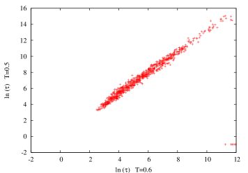
Figure 6: Logarithm of the relaxation time for $T=0.5$ as a function of the logarithm of the relaxation time for the same disorder sample $J$ but $T=0.6$. The number of sites is $N=64$. There are a couple of disorder samples with $\tau>t_{window}$ for $T=0.5$ in this figure. Those are the points with $\ln{\tau}=-1$ (by convention).

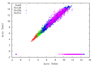
Figure 7: (Colour on line) Same as in figure 6 but with $N=64,128,256$ and $512$ together. There are a couple of disorder samples with $\tau>t_{window}$ for both $T=0.5$ and $T=0.6$ in this figure. Those are the points with $\ln{\tau}=-1$ (by convention).

In conclusion, we have measured the equilibrium relaxation time $\tau$ of the Sherrington-Kirkpatrick model with binary couplings for many samples of the quenched disorder, and several values of the temperature, with system sizes from $N=64$ to $512$, taking great care that the thermal noise is negligible. We confirm the result of [4] that the slow samples are not correlated to “ferromagnetic” disorder configurations, but we did not find evidence for a dominance by configurations with a small value at the origin of the site averaged local field probability distribution. We find a strong correlation between the relaxation times measured at two distinct values of the temperature (with the same disorder sample). Closer look shows a broadening as $N$ grows, that is possibly an indication of the onset of temperature chaos.

References

- [1] D. Sherrington, and S. Kirkpatrick: Phys. Rev. Lett. 35 1792 (1975); Phys. Rev. B 17, 4384 (1978).
- [2] A. Billoire, and E. Marinari: J. Phys. A Math. Gen. 34, L727 (2001).
- [3] A. Billoire: J. Stat. Mech. P11034 (2010) arXiv:1003.6086 [cond-mat].
- [4] C. Monthus, and T. Garel: J. Stat. Mech. P12017 (2009).
- [5] E. Bittner, and W. Janke: Europhys. Lett. 74, 195 (2006).
- [6] B.A. Berg, A. Billoire, and W. Janke: Phys. Rev. B 61 12143 (2000).
- [7] R. Alvarez Baños et al. (Janus collaboration): J. Stat. Mech. P06026 (2010).
- [8] G. J. Rodgers, and M. A. Moore: J. Phys. A: Math. Gen. 22, 1085 (1989).
- [9] T. Aspelmeier, A. Billoire, E. Marinari, and M.A.Moore: J. Phys. A 41, 324008 (2008).
- [10] M. Thomsen, M.F. Thorpe, T.C. Choy, D. Sherrington, and H.-J. Sommers: Phys. Rev. B 33, 1931 (1986).