Time Reversal of Some Stationary Jump-Diffusion Processes
from Population Genetics

Abstract

We describe the processes obtained by time reversal of a class of stationary jump-diffusion processes that model the dynamics of genetic variation in populations subject to repeated bottlenecks. Assuming that only one lineage survives each bottleneck, the forward process is a diffusion on $[0,1]$ that jumps to the boundary before diffusing back into the interior. We show that the behavior of the time-reversed process depends on whether the boundaries are accessible to the diffusive motion of the forward process. If a boundary point is inaccessible to the forward diffusion, then time reversal leads to a jump-diffusion that jumps immediately into the interior whenever it arrives at that point. If, instead, a boundary point is accessible, then the jumps off of that point are governed by a weighted local time of the time-reversed process.

1 Introduction

Kingman’s observation that the genealogy of a random sample of individuals from a panmictic, neutrally-evolving population can be represented as a Markov process [16, 17] ranks as one of the most influential contributions of mathematical population genetics. Not only has the coalescent led to a deeper understanding of evolution in neutral populations, but it also plays a central role in statistical genetics where it facilitates the efficient simulation of sample genealogies. Unfortunately, the Markov property that makes Kingman’s coalescent both mathematically and computationally tractable is usually not shared by genealogical processes in populations composed of non-exchangeable individuals. In particular, this is true when there are fitness differences between individuals, since then the selective interactions between individuals cause genealogies to depend on the history of lineages that are non-ancestral to the sample. The key to overcoming this difficulty is to extend the genealogy to a higher-dimensional process that does satisfy the Markov property. This has been done in two ways. One approach is to embed the genealogical tree within a graphical process called the ancestral selection graph [18, 24, 6] in which lineages can both branch and coalesce. The intuition behind this construction is that the effects of selection on the genealogy can be accounted for by keeping track of a pool of potential ancestors which includes lineages that have failed to persist due to being out-competed by individuals of higher fitness.

An alternative approach was proposed by Kaplan et al. (1988) [12], who showed that the genealogical history of a sample of genes under selection can be represented as a structured coalescent process. Here we think of the population as being divided into several panmictic subpopulations (called genetic backgrounds) which consist of individuals that share the same genotype at the selected locus. Because individuals with the same genotype are exchangeable (i.e., they have the same fitness), the rate of coalescence within a background depends only on the size of the background and the number of ancestral lineages sharing that genotype. Thus, to obtain a Markov process, we need to keep track of two kinds of information: (i) the types of the ancestral lineages, and (ii) the frequencies of the alleles segregating at the selected locus, followed backwards in time. For many applications it is assumed that the population is at equilibrium and that the forwards in time dynamics of the allele frequencies are described by a stationary diffusion process. In this case, the ancestral process of allele frequencies can be identified by time reversal of the diffusion process. In particular, if the diffusion process is one-dimensional, then the time-reversed process conveniently has the same law as the forward process. A formal derivation of the structured coalescent process for such an equilibrium population is given in [2] and various applications are discussed in [1, 5, 30].

The focus of this article is on the time reversal of a population genetical model that incorporates mutation, selection, genetic drift and population bottlenecks. To be concrete, consider a locus with two alleles, $A_{0}$ and $A_{1}$, and let $p^{N}(t)$ denote the frequency of $A_{1}$ at time $t$ in a population of size $N$. In the absence of bottlenecks, we will suppose that the jump process $p^{N}(\cdot)$ can be approximated by the Wright-Fisher diffusion $p(\cdot)$ with generator

$$\begin{split}A\phi(p)&=\frac{1}{2}p(1-p)\phi^{\prime\prime}(p)+(\mu_{0}(1-p)-\mu_{1}p+s(p)p(1-p))\phi^{\prime}(p)\\ &\equiv\frac{1}{2}v(p)\phi^{\prime\prime}(p)+\mu(p)\phi^{\prime}(p),\end{split}$$ (1)

where $\mu_{0}$ and $\mu_{1}$ are the scaled mutation rates from $A_{0}$ to $A_{1}$ and from $A_{1}$ to $A_{0}$, respectively, and $s(p)$ is the scaled and possibly frequency-dependent selection coefficient of $A_{1}$ relative to $A_{0}$. In using the diffusion approximation, we assume that $N$ is large, that time is measured in units of $N$ generations, and the unscaled mutation rates and selection coefficient are of order $N^{-1}$. Convergence results justifying the passage to the diffusion limit can be found in [7].

Population bottlenecks are transient events during which most of the population is descended from a small number of individuals. On the diffusive time scale, these can be modeled as instantaneous jumps in the allele frequencies, and in this article we will be concerned with a class of models in which the bottlenecks always result in the temporary fixation of one of the two alleles, i.e., $p(\cdot)$ always jumps to $0$ or $1$. We have two scenarios in mind. In the first, we consider a locus that is part of a non-recombining segment of DNA (e.g., a mammalian mitochondrial genome) subject to strong selective sweeps which occur at rate $\lambda$. During each sweep, a unique copy of a favorable mutation arises at some linked site and rises rapidly to fixation. Depending on whether the new, strongly-selected mutation occurs on a chromosome carrying an $A_{1}$ or $A_{2}$ allele, the frequency of $A_{1}$ will either increase from $p$ to $1$ with probability $p$ or decrease from $p$ to $0$ with probability $1-p$. Here we imagine that the selective advantage of the favored mutation is so strong that this change can be treated as a jump. The pseudohitchhiking model introduced by Gillespie [10] belongs to this class, as does a related, more general model studied by Kim [15].

The second scenario concerns demographic bottlenecks that occur during transmission of parasites from infected to uninfected hosts. Here we will let $p$ denote the frequency of $A_{1}$ in a chronological series of infected hosts linked by a transmission chain, and we will assume that $p(\cdot)$ can be modeled by a diffusion process from the time when one of these hosts is first infected to the time when that host first transmits the infection to the next host in the transmission chain. Suppose that transmissions occur at rate $\lambda$, and that each new infection is founded by a single parasite, as has been proposed for HIV-1 [31] and for some bacterial pathogens [29]. In this case, $p$ will jump to $0$ or $1$ following each transmission depending on the type of the transmitted parasite. Also, to allow for the possibility that transmission itself might be selective (e.g., [27]), we will let $w(p)$ denote the probability that the transmitted parasite is of type $A_{1}$ given that the frequency of this allele in the transmitting host is $p$. In general, we stipulate that $w(0)=0$, $w(1)=1$, and that $w(p)$ is monotonically increasing. If transmission is unbiased, then $w(p)=p$, as in the pseudohitchhiking model. A particular case of this transmission chain model was studied by Rouzine and Coffin [28] to understand the effects of selection and transmission bottlenecks on antigenic variation in HIV-1.

Both of these scenarios can be modeled by a jump-diffusion process with infinitesimal generator

$$\begin{split}G\phi(p)=&\frac{1}{2}p(1-p)\phi^{\prime\prime}(p)+(\mu_{0}(1-p)-\mu_{1}p+s(p)p(1-p))\phi^{\prime}(p)+\\ &\lambda w(p)\big{(}\phi(1)-\phi(p)\big{)}+\lambda(1-w(p))\big{(}\phi(0)-\phi(p)\big{)},\end{split}$$ (2)

where for technical reasons we will assume that $s(p)$ and $w(p)$ are smooth functions on $[0,1]$, and that both mutation rates, $\mu_{0}$ and $\mu_{1}$, are positive. Under these conditions, it can be shown (cf. Lemma 3.1) that the process $p(\cdot)$ has a unique stationary distribution, $\pi(p)dp$, which has a density on $[0,1]$. To characterize the structured coalescent process corresponding to this model, we need to identify the stationary time reversal of the process $p(\cdot)$. Formally, this can be done by solving the following adjoint problem for the operator $\tilde{G}$:

$$\int_{0}^{1}\psi(p)G\phi(p)\pi(p)dp=\int_{0}^{1}\phi(p)\tilde{G}\psi(p)\pi(p)dp,$$ (3)

where $\phi$ is in the domain of $G$. If $\tilde{G}$ generates a Markov process $\tilde{p}(\cdot)$, then this process will have the same law as the stationary time reversal of $p(\cdot)$ [23]. When $\lambda=0$, $p(\cdot)$ is a diffusion process and a simple calculation using integration-by-parts shows that $\tilde{G}=G$, demonstrating that the law of the diffusion is invariant under time-reversal, as remarked above. However, if $\lambda>0$, then for the adjoint condition (3) to be satisfied for all $\phi\in\mathcal{C}^{2}(\mathbb{R})\cap\mathcal{C}[0,1]$, we must instead set

$$\tilde{G}\psi(p)=\frac{1}{2}p(1-p)\psi^{\prime\prime}(p)+{\tilde{\mu}}(p)\psi^{\prime}(p),$$ (4)

where

$${\tilde{\mu}}(p)=\frac{1}{\pi(p)}\big{(}p(1-p)\pi^{\prime}(p)+(1-2p-\mu(p))\pi(p)\big{)}$$ (5)

and $\psi\in\mathcal{C}^{2}(\mathbb{R})\cap\mathcal{C}[0,1]$ satisfies

$$\psi(1)=\int_{0}^{1}\psi(p)\left(\frac{w(p)\pi(p)}{\kappa}\right)dp\mbox{\;\;\; and \;\;\;}\psi(0)=\int_{0}^{1}\psi(p)\left(\frac{(1-w(p))\pi(p)}{1-\kappa}\right)dp$$

with $\kappa=\int_{0}^{1}w(p)\pi(p)dp$. Although it is not immediately clear that the operator defined by (4) is the generator of a Markov process, this calculation does show that the process incorporating bottlenecks is not invariant under time reversal.

To gain some insight into the qualitative behavior of the time-reversed process, it is useful to consider two heuristic descriptions. We begin by observing that the behavior of $\tilde{p}(\cdot)$ depends strongly on whether the boundary points $\{0,1\}$ are accessible or inaccessible to the diffusive motion of the forward process. Recall that for the Wright-Fisher diffusion corresponding to $A$ (which we call the diffusive motion of the jump-diffusion process), Feller’s boundary classification conditions show that $0$ (resp. $1$) is accessible if and only if $u_{0}<1/2$ (resp. $u_{1}<1/2$), see e.g. Section 4.7 in [8]. The importance of this distinction is illustrated in Figure 1, which shows sample paths of the jump-diffusion process corresponding to cases where the two boundaries are either inaccessible (A) or accessible (B) to the forward diffusion. To see what this suggests about the behavior of the time-reversed process, begin at the top of each figure and follow the sample path backwards in time towards the bottom. If the boundaries are inaccessible, then whenever the sample path is followed back to a boundary at some time, the forward process will necessarily have reached that boundary via a jump. Consequently, the time-reversed process must immediately jump into the interval $(0,1)$ whenever it arrives at a boundary that is inaccessible to the forward diffusion. The behavior of the time-reversed process at a boundary that is accessible to the forward diffusion is very different. In this case, when the sample path of the time-reversed jump diffusion hits that boundary, the forward process may have arrived there either diffusively or via a jump from the interior (Figure 1B). Accordingly, the time-reversed process need not immediately jump into the interior $(0,1)$ when it visits the boundary, although jumps can only occur when the process is on the boundary and are certain to occur at some such times if $\lambda>0$.

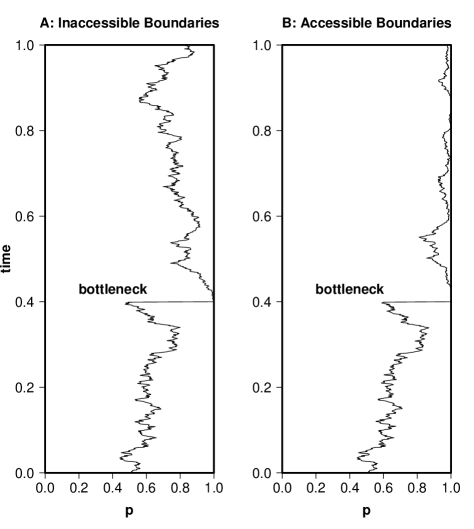
Figure 1: Sample paths of the jump-diffusion process (2) with either inaccessible (A) or accessible boundaries (B). The forward diffusion is a neutral Wright-Fisher process with symmetric mutation: $\mu_{0}=\mu_{1}=1$ in A and $0.2$ in B.

A more quantitative picture of this second case can be obtained by considering a less singular process that approximates the jump-diffusion process corresponding to (2). For $\epsilon\in(0,1/2)$, let $p_{\epsilon}(\cdot)={{\bigl{(}p_{\epsilon}(t):t\geq 0\bigr{)}}}$ be a perturbation of a Wright-Fisher diffusion which at rate $\lambda$ jumps to a point chosen uniformly at random from an interval of width $\epsilon$ adjacent to one of the two boundaries. More precisely, let $p_{\epsilon}(\cdot)$ be the Markov process with generator

$$G_{\epsilon}\phi(p) = \frac{1}{2}p(1-p)\phi^{\prime\prime}(p)+\big{(}\mu_{0}(1-p)-\mu_{1}p+s(p)p(1-p)\big{)}\phi^{\prime}(p)+$$

$$\lambda\left(w(p)\frac{1}{\epsilon}\int_{1-\epsilon}^{1}(\phi(q)-\phi(p))dq+(1-w(p))\frac{1}{\epsilon}\int_{0}^{\epsilon}(\phi(q)-\phi(p))dq\right).$$

Writing $\pi_{\epsilon}(p)$ for the density of the stationary distribution of this process, a simple calculation using (3) shows that the stationary time reversal of $p_{\epsilon}(\cdot)$, denoted $\tilde{p}_{\epsilon}(\cdot)$, is also a jump diffusion process with generator

$$\tilde{G}_{\epsilon}\psi(p) = \frac{1}{2}p(1-p)\psi^{\prime\prime}(p)+\frac{1}{\pi_{\epsilon}(p)}\big{(}p(1-p)\pi_{\epsilon}^{\prime}(p)+(1-2p-\mu(p))\pi_{\epsilon}(p)\big{)}\psi^{\prime}(p)+$$

$$\lambda\kappa_{\epsilon}\left(\frac{1}{\epsilon\pi_{\epsilon}(p)}1_{(1-\epsilon,1]}(p)\right)\int_{0}^{1}\left(\frac{w(q)\pi_{\epsilon}(q)}{\kappa_{\epsilon}}\right)(\psi(q)-\psi(p))dq+$$

$$\lambda(1-\kappa_{\epsilon})\left(\frac{1}{\epsilon\pi_{\epsilon}(p)}1_{[0,\epsilon)}(p)\right)\int_{0}^{1}\left(\frac{(1-w(q))\pi_{\epsilon}(q)}{1-\kappa_{\epsilon}}\right)(\psi(q)-\psi(p))dq,$$

where $\psi\in\mathcal{C}^{2}([0,1])$ and $\kappa_{\epsilon}=\int_{0}^{1}w(p)\pi_{\epsilon}(p)dp$. It is easy to read off the behavior of this process from its generator. In particular, we see that $\tilde{p}_{\epsilon}(\cdot)$ can only jump when it is present in the region $[0,\epsilon)\cup(1-\epsilon,1]$ and that the rate at which jumps occur out of this region is equal to $\lambda\kappa_{\epsilon}/(\epsilon\pi_{\epsilon}(p))$ when $p\in(1-\epsilon,1]$ and $\lambda(1-\kappa_{\epsilon})/(\epsilon\pi_{\epsilon}(p))$ when $p\in[0,\epsilon)$.

To relate these observations to the process $\tilde{p}(\cdot)$, let $T>0$ and notice that as $\epsilon$ tends to $0$, the sequence of processes $(p_{\epsilon}(\cdot))$ converges in distribution on $D_{[0,1]}([0,T])$ to $p(\cdot)$. Furthermore, because time reversal is a continuous mapping on $D_{[0,1]}([0,T])$, the continuous mapping theorem [7] implies that the sequence of processes $(\tilde{p}_{\epsilon}(\cdot))$ converges in distribution to the process $\tilde{p}(\cdot)$. In particular, this suggests that $\tilde{p}(\cdot)$ has the following behavior. For each $\epsilon\in(0,1/2)$, define the additive functionals

$$L_{1,\epsilon}(t) \equiv \frac{1}{\epsilon}\int_{0}^{t}\left(\frac{1}{\pi(\tilde{p}(s))}\right)1_{(1-\epsilon,1]}(\tilde{p}(s))ds$$

$$L_{0,\epsilon}(t) \equiv \frac{1}{\epsilon}\int_{0}^{t}\left(\frac{1}{\pi(\tilde{p}(s))}\right)1_{[0,\epsilon)}(\tilde{p}(s))ds,$$

and suppose that for $i=0,1$, the limits $L_{i}(t)=\lim_{\epsilon\rightarrow 0}L_{i,\epsilon}(t)$ exist for all $t\geq 0$. Here we would like to interpret $L_{i}(t)$ as the local time of the process $\tilde{p}(\cdot)$ at $i\in\{0,1\}$. Then, by comparison with the jump-diffusion processes $\tilde{p}_{\epsilon}(\cdot)$, we expect that if both boundaries are accessible, then $\tilde{p}(\cdot)$ is a jump-diffusion with diffusive motion in $(0,1)$ governed by (4) which jumps from the boundary point $0$ to a random point in the interval $(0,1)$ distributed as $\tfrac{1}{\kappa}w(q)\pi(q)\,dq$ as soon as $L_{0}(\cdot)$ exceeds an exponential random variable with parameter ${\lambda}\kappa$ and which jumps from the boundary point $1$ to a random point distributed as $\tfrac{1}{1-\kappa}{{\bigl{(}1-w(q)\bigr{)}}}\pi(q)\,dq$ on $(0,1)$ as soon as $L_{1}(\cdot)$ exceeds an exponential random variable with parameter ${\lambda}(1-\kappa)$. Although these remarks are purely heuristic, we show below that they correctly describe the stationary time reversal of the pseudo-hitchhiking model and other jump-diffusions with generators of the form (2).

2 Main result

Although our principle concern is with the modified Wright-Fisher process corresponding to (2), we state our results for a more general class of jump-diffusion processes, which we now introduce. Let the forward process ${{\bigl{(}p(t)\colon t\geq 0\bigr{)}}}$ be the jump-diffusion process on $[0,1]$ corresponding to the generator

$$\begin{split}G\phi(p)=\tfrac{1}{2}v(p)\phi^{\prime\prime}(p)+\mu(p)\phi^{\prime}(p)+\lambda w_{0}(p)\big{(}\phi(0)-\phi(p)\big{)}+\lambda w_{1}(p)\big{(}\phi(1)-\phi(p)\big{)},\end{split}$$ (6)

for $\phi\in{\mathbf{C}}^{2}{{\bigl{(}[0,1]\bigr{)}}}$. In other words, the diffusive motion of $p(\cdot)$ is governed by the generator

$$A\phi(p)=\tfrac{1}{2}v(p)\phi^{\prime\prime}(p)+\mu(p)\phi^{\prime}(p),\quad\phi\in{\mathbf{C}}^{2}{{\bigl{(}[0,1]\bigr{)}}},$$ (7)

with infinitesimal drift and variance coefficients, $\mu(\cdot)$ and $v(\cdot)$, respectively, while jumps occur at constant rate ${\lambda}\geq 0$ and move the process from state $p\in[0,1]$ either to $0$ with probability $w_{0}(p)\in[0,1]$ or to $1$ with probability $w_{1}(p):=1-w_{0}(p)$. Throughout this article, we will assume that the following conditions are satisfied.

Assumption 2.1.

The infinitesimal mean and variance satisfy $\mu(0)>0>\mu(1)$ and $v(0)=v(1)=0<v(p)$ for all $p\in(0,1)$, respectively. Furthermore, $v(\cdot)$, $\mu(\cdot)$ and $w_{0}(\cdot)$ are analytic functions in a neighborhood of $[0,1]$, and the infinitesimal variance has non-zero derivatives $v^{{}^{\prime}}(0)>0>v^{{}^{\prime}}(1)$ at the boundaries.

For example, if $A$ is the generator of a neutral Wright-Fisher diffusion (1) (with $s(p)\equiv 0$), then Assumption 2.1 is satisfied with $\mu(0)=\mu_{0}>0$, $\mu(1)=-\mu_{1}<0$, and $v^{{}^{\prime}}(0)=1=-v^{{}^{\prime}}(1)$. We also remark that when Assumption 2.1 is satisfied, Lemma 3.1 shows that ${{\bigl{(}p(t)\colon t\geq 0\bigr{)}}}$ has a unique stationary distribution $\pi(p)dp$ with a density $\pi(\cdot)$ that satisfies a second order ordinary differential equation with non-local boundary conditions.

In Theorem 2.1, we characterize the time-reversed process ${{\bigl{(}{\tilde{p}}(t)\colon t\geq 0\bigr{)}}}$ of the forward process ${{\bigl{(}p(t)\colon t\geq 0\bigr{)}}}$. In keeping with the heuristic description given in the Introduction, ${{\bigl{(}{\tilde{p}}(t)\colon t\geq 0\bigr{)}}}$ is also a jump-diffusion process on $[0,1]$ but now with jumps from the boundary $\{0,1\}$ to the interior $(0,1)$. The diffusive motion of this process is governed by the generator

$${\tilde{A}}\psi(p)=\tfrac{1}{2}v(p)\psi^{\prime\prime}(p)+{\tilde{\mu}}(p)\psi^{\prime}(p)\qquad\text{where}\ \ {\tilde{\mu}}(p):=-\mu(p)+\frac{(v\pi)^{{}^{\prime}}(p)}{\pi(p)}$$ (8)

and $\psi\in{\mathbf{C}}^{2}{{\bigl{(}[0,1]\bigr{)}}}$. Notice that this diffusion has the same infinitesimal variance as the forward diffusion, but has a different infinitesimal drift that depends on the jump events via the stationary density $\pi(\cdot)$. Also, the jump rates of the time-reversed process depend on a local time process which is described in the following way. Recall that the scale function and the speed measure associated with ${\tilde{A}}$ are

$${\tilde{S}}(p):=\int_{\frac{1}{2}}^{p}\exp{{\Bigl{(}-\int_{\frac{1}{2}}^{x}\frac{2{\tilde{\mu}}(z)}{v(z)}\,dz\Bigr{)}}}dx\ \text{ and }\ {\tilde{m}}(dp):=\frac{1}{v(p){\tilde{S}}^{{}^{\prime}}(p)}dp,\quad p\in[0,1],$$ (9)

respectively. The scale function will be identified with the associated measure ${\tilde{S}}(dp):={\tilde{S}}^{{}^{\prime}}(p)dp$ on $[0,1]$ and the speed measure ${\tilde{m}}(dp)$ will be identified with its density function.

We define the local time process of the jump-diffusion ${\tilde{p}}(\cdot)$ such that it agrees with the local time process of the diffusive motion until the first jump. More formally, we will introduce a non-negative process ${{\bigl{(}{\tilde{L}}_{p}(t)\colon t\geq 0,\,p\in[0,1]\bigr{)}}}$ which is almost surely continuous in $(t,p)$ and which satisfies

$$\int_{0}^{t}f{{\bigl{(}{\tilde{p}}(u)\bigr{)}}}\,du=\int_{0}^{1}f(p){\tilde{L}}_{p}(t)\,{\tilde{m}}(dp)\qquad\text{a.s.}\ t\geq 0$$ (10)

for all measurable $f\colon[0,1]\to[0,\infty)$. We remark that the local time process satisfying (10) differs from the semi-martingale local time of the diffusive motion of the time-reversed process by a scalar factor (see Eq. (77)), i.e., ${\tilde{L}}$ is a weighted semi-martingale local time. That this process is well-defined is shown below in Lemma 6.1. The last ingredient needed in our construction is a pair of independent, exponentially-distributed random variables, $R_{0}$ and $R_{1}$, with parameters

$$r_{i}:=\lim_{p\to i}{{\Bigl{(}\frac{{\tilde{m}}(p)}{\pi(p)}\lambda\kappa_{i}\Bigr{)}}}\in[0,\infty]$$ (11)

where $\kappa_{i}:=\int_{0}^{1}w_{i}(p)\pi(p)dp$, $i\in\{0,1\}$. The existence of the limit displayed in (11) is guaranteed by Lemma 4.3. By convention, $R_{i}:=0$ if $r_{i}=\infty$ and $R_{i}:=\infty$ if $r_{i}=0$.

With these definitions, we now describe the dynamics of the time-reversed process ${{\bigl{(}{\tilde{p}}(t)\colon t\geq 0\bigr{)}}}$. Between jump times, ${{\bigl{(}{\tilde{p}}(t)\colon t\geq 0\bigr{)}}}$ evolves according to the law of the diffusion governed by ${\tilde{A}}$. If this diffusion hits a boundary $i\in\{0,1\}$ at a time $t\geq 0$ and if at that time the local time process exceeds the random variable $R_{i}$, that is, if ${\tilde{L}}_{i}(t)\geq R_{i}$, then ${\tilde{p}}(\cdot)$ jumps from $i$ to a random point chosen from $(0,1)$ according to the distribution $\tfrac{1}{\kappa_{i}}\int w_{i}(p)\pi(p)dp$. From this point, ${\tilde{p}}(\cdot)$ restarts independently of the sample path up to that time.

To better understand how the dynamics of ${\tilde{p}}(\cdot)$ are influenced by the boundary behavior of the forward process, we take a closer look at the jump times. Because the coefficients $v(\cdot)$ and $\mu(\cdot)$ are smooth on an interval containing $[0,1]$, an application of Feller’s boundary classification criteria shows that a boundary point $i\in\{0,1\}$ is accessible to the forward diffusive motion if and only if $2{|\mu(i)|}<{|v^{{}^{\prime}}(i)|}$. Then, in conjunction with Lemma 3.2, which describes the asymptotics of the density $\pi(p)$ near the boundaries, Lemma 4.3 implies that

$$r_{i}:=\lim_{p\to i}{{\Bigl{(}\frac{{\tilde{m}}(p)}{\pi(p)}\lambda\kappa_{i}\Bigr{)}}}\left\{\begin{array}[]{ll}\in(0,\infty)&\mbox{ \; if $2{|\mu(i)|}<{|v^{{}^{\prime}}(i)|}$ and $\lambda w_{i}(\cdot)\not\equiv 0$ }\\ =\infty&\mbox{ \; if $2{|\mu(i)|}\geq{|v^{{}^{\prime}}(i)|}$ and $\lambda w_{i}(\cdot)\not\equiv 0$}\\ =0&\mbox{ \; if $\lambda w_{i}(\cdot)\equiv 0$}\end{array}\right.$$ (12)

for $i\in\{0,1\}$. Thus, provided that $\lambda w_{i}(\cdot)\not\equiv 0$, the time-reversed process immediately jumps into the interior $(0,1)$ if the boundary point is inaccessible to the forward diffusive motion, that is, if $2{|\mu(i)|}\geq{|v^{{}^{\prime}}(i)|}$. In this case, the state space of ${\tilde{p}}(\cdot)$ is in fact $[0,1]\setminus\{i\}$. In contrast, if $i$ is accessible to the forward diffusion and $\lambda w_{i}(\cdot)>0$, then the exponential random variable $R_{i}$ is almost surely positive and so a positive amount of local time will have to be accrued at $i$ before a jump occurs off of this boundary point.

Notice that, in either case, we expect that both boundary points are accessible to the backward diffusive motion. According to Lemma 4.1

$${\tilde{\mu}}(i)=\left\{\begin{array}[]{ll}\mu(i)&\mbox{ \; if $2{|\mu(i)|}\leq{|v^{{}^{\prime}}(i)|}$}\\ v^{{}^{\prime}}(i)-\mu(i)&\mbox{ \; if $2{|\mu(i)|}\geq{|v^{{}^{\prime}}(i)|}$}\end{array}\right.,\quad i\in\{0,1\},$$ (13)

and again an application of Feller’s boundary criteria shows that the boundary point $i$ is accessible to the backward diffusive motion whenever $2\mu(i)\neq v^{{}^{\prime}}(i)$. The critical case is more subtle. Then, $2{\tilde{\mu}}(i)=v^{{}^{\prime}}(i)$, and so $i$ would be inaccessible if the drift coefficient ${\tilde{\mu}}(\cdot)$ were analytic in a neighborhood of $i$. However, we show in Lemma 4.1 that

$${\tilde{\mu}}(p)=\mu(i)+\frac{v^{{}^{\prime}}(i)}{\ln{{\bigl{(}|p-i|\bigr{)}}}}+O{{\bigl{(}\frac{{|p-i|}}{\ln{{|p-i|}}}\bigr{)}}},$$ (14)

and then Feller’s criteria reveal that the logarithmic singularity is just sufficient to render the point $i$ accessible to the backward diffusive motion when $2{\tilde{\mu}}(i)=v^{{}^{\prime}}(i)$.

Our main result states that the process ${\tilde{p}}(\cdot)$ has the same law as the stationary time reversal of the jump-diffusion $p(\cdot)$.

Theorem 2.1.

Assume 2.1. Let $p(\cdot)$ be the jump-diffusion on $[0,1]$ with generator $G$ as defined in (6). Then the process ${{\bigl{(}{\tilde{p}}(t)\colon t\geq 0\bigr{)}}}$ is a version of the stationary time reversal of ${{\bigl{(}p(t)\colon t\geq 0\bigr{)}}}$, that is,

$${{\bigl{(}{\tilde{p}}(t)\colon t\leq T\bigr{)}}}{\;\overset{d}{=}\;}{{\bigl{(}p(T-t)\colon t\leq T\bigr{)}}}\quad\;\;\forall\;T\geq 0$$ (15)

if the distribution of $p(0)$ is the stationary distribution $\pi(p)dp$.

The proof of Theorem 2.1 is deferred to Section 7.

Theorem 2.1 establishes the time reversal of the stationary process over a fixed time interval $[0,T]$, $T<\infty$ fixed and non-random. Readers being interested in other pathwise time reversals are referred to the literature. It has been shown that processes which are in ’Hunt duality’ (see [4, Chapter VI]) are time reversals of each other. Reversing time at the end point of an excursion from an accessible boundary point results in the dual process being started at this boundary point, see [9, 21]. The paper of Mitro [22] reverses time at inverse local time points.

The remainder of the paper is organized as follows. The next section collects some results concerning the stationary distribution of the jump-diffusion process (2). Section 4 describes the boundary behavior of ${\tilde{p}}(\cdot)$. In particular we show that the time-reversed process jumps immediately off of any boundary that is inaccessible to the forward diffusion. In Section 5 we identify a core for the generator $\tilde{G}$ satisfying the adjoint condition (3). The local time process of ${\tilde{p}}(\cdot)$ is introduced and studied in Section 6. Finally, Section 7 shows that ${\tilde{p}}(\cdot)$ has generator ${\tilde{G}}$. The proof of this result depends on an application of the Itô-Tanaka formula.

3 The stationary distribution

The following lemma asserts that, if the conditions of Assumption 2.1 are satisfied, then the jump-diffusion process $p(\cdot)$ has a unique stationary distribution on $[0,1]$. It is also shown that this distribution has a density $\pi(\cdot)$ with respect to Lebesgue measure which satisfies a second-order ordinary differential equation (ODE) subject to boundary conditions that are non-local whenever ${\lambda}>0$. If ${\lambda}=0$, then this equation can be solved explicitly, leading to the familiar expression

$$\pi(p)=C^{-1}\frac{1}{v(p)}\exp\Big{(}2\int^{p}\mu(q)/v(q)dq\Big{)},$$ (16)

where $C$ is a normalizing constant, e.g., see Section 4.5 in [8]. Although a general closed-form expression for $\pi(\cdot)$ apparently does not exist when ${\lambda}>0$, $\pi(\cdot)$ can be calculated by numerically solving (17) using a modification of the shooting method [25]. In addition, below we give an explicit formula for the stationary density in the important special case of a neutral Wright-Fisher diffusion subject to recurrent bottlenecks.

Lemma 3.1.

Assume 2.1. Then there exists a unique stationary distribution for the process ${{\bigl{(}p(t)\colon t\geq 0\bigr{)}}}$. This distribution is given by ${\mathbbm{1}}_{(0,1)}(p)\pi(p)dp$ where $\pi\colon(0,1)\to(0,\infty)$ is the unique solution of the non-local boundary value problem

$$\begin{split}{{\bigl{(}(\tfrac{1}{2}v\pi)^{{}^{\prime\prime}}-(\mu\pi)^{{}^{\prime}}-\lambda\pi\bigr{)}}}(p)&=0\quad\;\;\forall\;p\in(0,1)\\ \lim_{p\to 0}{{\bigl{(}\mu\pi-(\tfrac{1}{2}v\pi)^{{}^{\prime}}\bigr{)}}}(p)&={\lambda}\kappa_{0}\\ \lim_{p\to 1}{{\bigl{(}\mu\pi-(\tfrac{1}{2}v\pi)^{{}^{\prime}}\bigr{)}}}(p)&=-{\lambda}\kappa_{1}\\ \lim_{p\to 0}(v\pi)(p)&=0=\lim_{p\to 1}(v\pi)(p)\\ \int_{0}^{1}\pi(p)dp&=1,\end{split}$$ (17)

where $\kappa_{i}:=\int_{0}^{1}w_{i}(p)\pi(p)dp$ for $i\in\{0,1\}$. Furthermore $p(t)$ converges in distribution to the stationary distribution as $t\to\infty$ for every initial distribution of $p(0)$.

Proof.

Existence and uniqueness of a stationary distribution ${\bar{\pi}}(dp)$ follow from standard arguments, so we only give a sketch. Couple two versions of ${{\bigl{(}p(t)\colon t\geq 0\bigr{)}}}$ with different initial distributions through the same jump times such that the diffusive motions in between jumps are independent until they first meet and are identical thereafter. Due to the assumption $\mu(0)>0>\mu(1)$, the coupling is successful if there are no jumps, that is, if $\lambda=0$, see Theorem V.54.5 in [26]. In the presence of jumps $(\lambda>0)$, the probability that both components jump to the same boundary is positive at every jump and, therefore, the two components agree eventually. As a consequence of this successful coupling and of compactness of $[0,1]$, $p(t)$ converges in distribution to a probability measure ${\bar{\pi}}(dp)$ as $t\to\infty$ and ${\bar{\pi}}(dp)$ is an invariant distribution.

Next we prove that ${\bar{\pi}}(\cdot)$ has a smooth density $\pi(\cdot)$. Denote by $(X(t))_{t\geq 0}$ the diffusion governed by $A$ (see (1)). The scale function and the speed measure associated with $A$ are

$$S(p):=\int_{\frac{1}{2}}^{p}\exp{{\Bigl{(}-\int_{\frac{1}{2}}^{x}\frac{2\mu(z)}{v(z)}\,dz\Bigr{)}}}dx\ \text{ and }\ m(p)dp:=\frac{1}{v(p)S^{{}^{\prime}}(p)}dp,\quad p\in[0,1],$$ (18)

respectively. Existence and smoothness of the density $\pi(\cdot)$ will be derived from existence and uniqueness of the transition density $Q(t;p,q)$ of $(X(t))_{t\geq 0}$ with respect to the speed measure. Existence of $Q(t;p,q)$ is established in Itô and McKean (1974) [11] ([20] is more detailed in a special case) via an eigen-differential expansion. To state this result more formally, we introduce the following notation. The interval defined in [11] – here denoted by $I^{\bullet}$ – is the unit interval closed at $0$ if $0$ is accessible, closed at $1$ if $1$ is accessible and open otherwise. For this, note that whenever $(X(t))_{t\geq 0}$ hits a boundary point, it immediately returns to the interior $(0,1)$ because of the assumption $\mu(0)>0>\mu(1)$. Moreover note that the stopping time $\min\{t\geq 0\colon X(t)\not\in I^{\bullet}\}=\infty$ is infinity almost surely. The generator of $(X(t))_{t\geq 0}$ is defined in [11] via right derivatives. As $(X(t))_{t\geq 0}$ is a regular diffusion, this generator coincides with

$$Af(p)=\frac{1}{m(p)}\frac{d}{dp}{{\Bigl{(}\frac{1}{S^{{}^{\prime}}(p)}f^{{}^{\prime}}(p)\Bigr{)}}}\qquad p\in I^{\bullet}$$ (19)

for $f\in{\mathbf{C}}^{2}(I^{\bullet})$. There exists a solution $\mathfrak{e}(\gamma,\cdot)={{\bigl{(}\mathfrak{e}_{1}(\gamma,\cdot),\mathfrak{e}_{2}(\gamma,\cdot)\bigr{)}}}$ of

$$\begin{split}{{\Bigl{(}A\mathfrak{e}{{\bigl{(}\gamma,\cdot\bigr{)}}}\Bigr{)}}}(p)&=\gamma\mathfrak{e}{{\bigl{(}\gamma,p\bigr{)}}}\qquad\;\;\forall\;0<p<1\\ \mathfrak{e}{{\bigl{(}\gamma,\tfrac{1}{2}\bigr{)}}}=(1,0)&\qquad\frac{1}{m(\tfrac{1}{2})}\mathfrak{e}^{{}^{\prime}}{{\bigl{(}\gamma,\tfrac{1}{2}\bigr{)}}}=(0,1)\end{split}$$ (20)

for every $\gamma\in(-\infty,0]$ such that $\gamma\mapsto\mathfrak{e}(\gamma,p)$ is continuous for every $p\in I^{\bullet}$. Based on these eigenfunctions, it is shown in [11] that there exists a Borel measure $\mathfrak{s}(d\gamma)$ from $(-\infty,0]$ to $2\times 2$ symmetric non-negative definite matrices

$$\mathfrak{s}(d\gamma)=\begin{pmatrix}\mathfrak{s}_{11}(d\gamma)&\mathfrak{s}_{12}(d\gamma)\\ \mathfrak{s}_{21}(d\gamma)&\mathfrak{s}_{22}(d\gamma)\end{pmatrix}$$ (21)

such that

$$Q(t;p,q)=\int_{-\infty}^{0}e^{\gamma t}\mathfrak{e}^{T}(\gamma,p){\displaystyle\cdot}\mathfrak{s}(d\gamma){\displaystyle\cdot}\mathfrak{e}(\gamma,p),\quad(t,p,q)\in(0,\infty)\times I^{\bullet}\times I^{\bullet},$$ (22)

is the transition density of $(X(t))_{t\geq 0}$ with respect to the speed measure $m(\cdot)$. Now as our jump diffusion $p(\cdot)$ could also jump to an inaccessible boundary, we need to extend $p\mapsto Q(t;p,q)$ onto $[0,1]$. Note that if $i\in\{0,1\}$ is inaccessible, then $i$ is an entrance boundary due to the assumption $(-1)^{i}\mu(i)>0$. As in Problem 3.6.3 in [11], one uses the Markov property to extend $(X(t))_{t\geq 0}$ to the state space $[0,1]$. Thus we may assume $Q(t;p,q)$ to be defined on $(0,\infty)\times[0,1]\times I^{\bullet}$.

With these results on the transition density of $(X(t))_{t\geq 0}$, we now establish existence of a smooth density of ${\bar{\pi}}(\cdot)$. Define $\kappa_{0}\in[0,1]$, $\kappa_{1}:=1-\kappa_{0}$ by

$$\kappa_{i}:=\int_{0}^{1}w_{i}(p){\bar{\pi}}(dp)\qquad\text{for }i\in\{0,1\}$$ (23)

and observe that $\kappa_{i}$ is the probability that a stationary version of the process jumps to the boundary point $i$ when it jumps. Recall that the jump times of $p(\cdot)$ form a Poisson process with rate $\lambda$ and that in between jumps, $p(\cdot)$ evolves according to $A$. If $U$ is any Borel measurable set in $[0,1]$, then by conditioning on the time and distribution of the last jump, we have

$${\bar{\pi}}(U)=\kappa_{0}\int_{0}^{\infty}\lambda e^{-\lambda t}\int_{U}Q(t;0,q)m(q)dq\,dt+\kappa_{1}\int_{0}^{\infty}\lambda e^{-\lambda t}\int_{U}Q(t;1,q)m(q)dq\,dt.$$

Interchanging integrals, we infer that ${\bar{\pi}}(\cdot)$ has a density with respect to Lebesgue measure and we set $\pi(q)dq:={\bar{\pi}}(dq)$ where $\pi\colon(0,1)\to[0,\infty)$ satisfies

$$\begin{split}\pi(q)&=\sum_{j=0}^{1}\kappa_{j}m(q)\int_{0}^{\infty}{\lambda}e^{-{\lambda}t}\int_{-\infty}^{0}e^{\gamma t}\mathfrak{e}^{T}(\gamma,j)\mathfrak{s}(d\gamma)\mathfrak{e}(\gamma,q)\,dt\\ &=\sum_{j=0}^{1}\kappa_{j}m(q)\int_{-\infty}^{0}\frac{\lambda}{\lambda-\gamma}\mathfrak{e}^{T}(\gamma,j)\mathfrak{s}(d\gamma)\mathfrak{e}(\gamma,q)\,dt\\ &=\lambda m(q){{\Bigl{(}\kappa_{0}G_{\lambda}(0,q)+\kappa_{1}G_{\lambda}(1,q)\Bigr{)}}}.\end{split}$$ (24)

The function $G_{\lambda}(p,q)$ is the Green’s function and is ${\mathbf{C}}^{2}$ in the second variable for every $p\in[0,1]$. As the speed density $m(\cdot)$ is also ${\mathbf{C}}^{2}$ in $(0,1)$ due to Assumption 2.1, we conclude that the stationary density $\pi(\cdot)$ is twice continuously differentiable.

The main step of the proof is to show that $\pi(\cdot)$ satisfies (17). By Proposition 4.9.2 of Ethier and Kurtz [7], the stationary distribution $\pi(p)dp$ satisfies

$$\int_{0}^{1}G\phi(p)\pi(p)dp=0$$ (25)

for all $\phi\in\mathbf{C}^{2}{{\bigl{(}[0,1]\bigr{)}}}$. Let $0<{\varepsilon}<\tfrac{1}{2}$. The functions $v,\mu,\phi$ and $\pi$ are $\mathbf{C}^{2}$ in $[{\varepsilon},1-{\varepsilon}]$. Integration by parts yields

$$\begin{split}\hbox to0.0pt{$\displaystyle\int_{\varepsilon}^{1-{\varepsilon}}G\phi{\displaystyle\cdot}\pi\,dp-\phi(0)\int_{\varepsilon}^{1-{\varepsilon}}\lambda w_{0}{\displaystyle\cdot}\pi\,dp-\phi(1)\int_{\varepsilon}^{1-{\varepsilon}}\lambda w_{1}{\displaystyle\cdot}\pi\,dp$\hss}\\ &=\int_{\varepsilon}^{1-{\varepsilon}}\phi^{{}^{\prime\prime}}{\displaystyle\cdot}(\tfrac{1}{2}v\pi)+\phi^{{}^{\prime}}{\displaystyle\cdot}(\mu\pi)-\lambda\phi\pi\,dp\\ &=[\phi^{{}^{\prime}}\tfrac{1}{2}v\pi]_{\varepsilon}^{1-{\varepsilon}}+[\phi{\displaystyle\cdot}{{\bigl{(}\mu\pi-(\tfrac{1}{2}v\pi)^{{}^{\prime}}\bigr{)}}}]_{\varepsilon}^{1-{\varepsilon}}-\int_{\varepsilon}^{1-{\varepsilon}}\phi{\displaystyle\cdot}{{\Bigl{[}(\mu\pi)^{{}^{\prime}}-(\tfrac{1}{2}v\pi)^{{}^{\prime\prime}}+\lambda\pi\Bigr{]}}}\,dp.\end{split}$$ (26)

By considering all functions $\phi\in\mathbf{C}^{2}$ with support in $({\varepsilon},1-{\varepsilon})$ and then letting ${\varepsilon}\to 0$, we conclude that $\pi(\cdot)$ satisfies the second-order ODE in (17). Furthermore, because the functions $G\phi$, $w_{0}$, $w_{1}$ are bounded and $\pi$ is integrable, we may apply the dominated convergence theorem to theintegrals on the left-hand side of (26) as ${\varepsilon}\to 0$. Together with (25) this shows that

$$\begin{split}{{\displaystyle\lim_{{\varepsilon}\rightarrow 0}}}&[\phi^{{}^{\prime}}\tfrac{1}{2}v\pi]_{\varepsilon}^{1-{\varepsilon}}+\phi(1){\displaystyle\cdot}{{\displaystyle\lim_{{\varepsilon}\rightarrow 0}}}{{\bigl{(}\mu\pi-(\tfrac{1}{2}v\pi)^{{}^{\prime}}\bigr{)}}}(1-{\varepsilon})-\phi(0){\displaystyle\cdot}{{\displaystyle\lim_{{\varepsilon}\rightarrow 0}}}{{\bigl{(}\mu\pi-(\tfrac{1}{2}v\pi)^{{}^{\prime}}\bigr{)}}}({\varepsilon})\\ &=-\phi(1)\lambda\kappa_{1}-\phi(0)\lambda\kappa_{0}.\end{split}$$ (27)

As $\phi$ was arbitrary this implies the non-local boundary conditions in (17).

If ${\hat{\pi}}(\cdot)$ is another normalized solution of (17), then reversing the previous arguments shows that (25) holds with $\pi$ replaced by ${\hat{\pi}}(\cdot)$. This in turn implies that ${\hat{\pi}}(p)dp$ is another stationary distribution and we conclude that ${\hat{\pi}}=\pi$. It remains to show that $\pi(\cdot)$ is strictly positive. Assuming $\pi(p)=0$ for some $p\in(0,1)$, we conclude that $\pi^{{}^{\prime}}(p)=0$ from $p$ being necessarily a global minimum. However, the only solution of the second-order ODE in (17) satisfying $\pi(p)=0=\pi^{{}^{\prime}}(p)$ is the zero function, which contradicts the assumption that $\pi(\cdot)$ is a probability density. ∎∎

Remark 3.1.

Lemma 3.1 can be used to find an explicit formula for $\pi(\cdot)$ when the jump-diffusion process is a model of a neutrally-evolving population subject to recurrent bottlenecks, i.e., when $p(\cdot)$ has generator

$$G\phi(p)=\frac{1}{2}p(1-p)\phi^{\prime\prime}(p)+(\mu_{0}(1-p)-\mu_{1}p)\phi^{\prime}(p)+\lambda\Big{(}p\phi(1)+(1-p)\phi(0)-\phi(p)\Big{)}.$$

In this case, (17) is a hypergeometric equation and, using the fact that the mean frequency of allele $A_{1}$ in a stationary population is $\mu_{0}/(\mu_{0}+\mu_{1})$, we find that the density $\pi(p)$ is equal to

$$\pi(p)=C^{-1}p^{2\mu_{0}-1}(1-p)^{2\mu_{1}-1}\Big{[}\mu_{0}F(1-a,1-b,2\mu_{0},p)+\mu_{1}F(1-a,1-b,2\mu_{1},1-p)\Big{]},$$

where $C$ is a normalizing constant, $F(a,b,c;z)$ is Gauss’ hypergeometric function, and the constants $a$ and $b$ are determined (up to interchange) by the equations $a+b=3-2(\mu_{0}+\mu_{1})$ and $ab=2(\lambda+1-\mu_{0}-\mu_{1})$.

The second lemma of this section provides information on the boundary behavior of the density of the stationary distribution. This information is derived using results on second-order ODEs with regular singular points.

We adopt the Landau big-O and little-o notation. In addition, for two functions $\psi_{1}(\cdot)$ and $\psi_{2}(\cdot)$, we write $\psi_{1}(p)\sim\psi_{2}(p)$ as $p\to i$ if both $\psi_{1}(p)=O{{\bigl{(}\psi_{2}(p)\bigr{)}}}$ and $\psi_{2}(p)=O{{\bigl{(}\psi_{1}(p)\bigr{)}}}$ as $p\to i$.

Lemma 3.2.

Assume 2.1. Let $\pi(\cdot)$ be the density of the stationary distribution of the jump-diffusion $p(\cdot)$ corresponding to the generator (6). Then, for $i\in\{0,1\}$, $\pi(\cdot)$ is equal to

$$\pi(p)=\left\{\begin{array}[]{ll}C_{i}{|p-i|}^{\frac{2\mu(i)-v^{{}^{\prime}}(i)}{v^{{}^{\prime}}(i)}}+O(1)&\mbox{if $2{|\mu(i)|}<{|v^{{}^{\prime}}(i)|}$}\\ \frac{2\lambda\kappa_{i}}{{|v^{{}^{\prime}}(i)|}}\ln{{\bigl{(}\frac{1}{|p-i|}\bigr{)}}}+O(1)&\mbox{if \ \,$2\mu(i)=v^{{}^{\prime}}(i)$ }\\ \frac{2\lambda\kappa_{i}}{{|2\mu(i)-v^{{}^{\prime}}(i)|}}+O{{\bigl{(}{|p-i|}+{|p-i|}^{\frac{2\mu(i)-v^{{}^{\prime}}(i)}{v^{{}^{\prime}}(i)}}\bigr{)}}}&\mbox{if $2{|\mu(i)|}>{|v^{{}^{\prime}}(i)|}$ and $\lambda w_{i}\not\equiv 0$}\\ C_{i}{|p-i|}^{\frac{2\mu(i)-v^{{}^{\prime}}(i)}{v^{{}^{\prime}}(i)}}+O{{\bigl{(}{|p-i|}^{\frac{2\mu(i)}{v^{{}^{\prime}}(i)}}\bigr{)}}}&\mbox{if $2{|\mu(i)|}>{|v^{{}^{\prime}}(i)|}$ and $\lambda w_{i}\equiv 0$}\end{array}\right.$$ (28)

as $p\to i$ where $C_{i}\in(0,\infty)$. In addition if $2\mu(i)=v^{{}^{\prime}}(i)$ and $\lambda w_{i}\equiv 0$, then $\pi(i)>0$.

Proof.

We only consider $i=0$ as the case $i=1$ is analogous. We begin by observing that $i=0$ is a regular singular point for the differential equation in (17), see e.g. Section 9.6 in [3] for this concept. The associated indicial equation for $0$ is

$$\nu(\nu-1)+2\frac{v^{{}^{\prime}}(0)-\mu(0)}{v^{{}^{\prime}}(0)}{\displaystyle\cdot}\nu=0$$ (29)

and has roots $\alpha:=0$ and $\beta:=\tfrac{2\mu(0)-v^{{}^{\prime}}(0)}{v^{{}^{\prime}}(0)}$. Note that $\beta>-1$. If ${\alpha}-\beta\not\in{\mathbbm{Z}}$, then Theorem IX.7 in [3] tells us that $\pi(\cdot)$ is equal to a linear combination of $b_{1}(p):=p^{\alpha}{{\bigl{(}1+h_{1}(p)\bigr{)}}}$ and $b_{2}(p):=p^{\beta}{{\bigl{(}1+h_{2}(p)\bigr{)}}}$ in a neighborhood of $0$ where $h_{1}$ and $h_{2}$ are suitable analytic functions satisfying $h_{1}(0)=0=h_{2}(0)$.

If ${\alpha}-\beta\in{\mathbbm{Z}}$, then Theorem IX.8 in [3] shows that $\pi(\cdot)$ is equal to a linear combination of $b_{1}(p)$, $b_{2}(p)$ and $\ln(p)b_{1}(p)$ in a neighborhood of $0$. If $2\mu(0)/v^{{}^{\prime}}(0)\in\mathbbm{N}_{\geq 2}$, then assuming $\pi(p)=-c_{1}\ln(p)+O(1)$, $\pi^{{}^{\prime}}(p)=-c_{1}\tfrac{1}{p}+O(1)$ for some constant $c_{1}>0$ leads to the contradiction

$$\infty>{\lambda}\kappa_{0}={{\bigl{(}\mu(0)-\tfrac{1}{2}v^{{}^{\prime}}(0)\bigr{)}}}\lim_{p\to 0}\pi(p)-\tfrac{1}{2}v^{{}^{\prime}}(0)\lim_{p\to 0}p\pi^{{}^{\prime}}(p)=\infty$$ (30)

where we have used (17). Therefore $\ln(p)$ does not contribute to $\pi(\cdot)$ if $2\mu(0)>v^{{}^{\prime}}(0)$.

It remains to calculate the coefficients. In the case $2\mu(0)\neq v^{{}^{\prime}}(0)$, insert $\pi(b)=c_{1}b_{1}(p)+c_{2}b_{2}(p)$ into (17) to obtain the coefficient $c_{1}$

$$\begin{split}\lambda\kappa_{0}&=\lim_{p\to 0}{{\Bigl{[}{{\bigl{(}\mu(p)-\frac{1}{2}v^{{}^{\prime}}(p)\bigr{)}}}\pi(p)-\frac{1}{2}v(p)\pi^{{}^{\prime}}(p)\Bigr{]}}}\\ &=\lim_{p\to 0}{{\Bigl{[}{{\bigl{(}\mu(0)-\frac{1}{2}v^{{}^{\prime}}(0)\bigr{)}}}{{\bigl{(}c_{1}+c_{2}p^{\beta}\bigr{)}}}-\frac{1}{2}v^{{}^{\prime}}(0)pc_{2}\beta p^{\beta-1}\Bigr{]}}}\\ &={{\bigl{(}\mu(0)-\frac{1}{2}v^{{}^{\prime}}(0)\bigr{)}}}c_{1}.\end{split}$$ (31)

Of course if $\lambda\kappa_{0}=0$, then $\pi(\cdot)\not\equiv 0$ implies $c_{2}>0$. Next we show that $\lambda\kappa_{0}>0$ together with $2\mu(0)<v^{{}^{\prime}}(0)$ implies $c_{2}>0$.

Assuming $c_{2}=0$ implies that $\pi(0)=\tfrac{2\lambda\kappa_{0}}{2\mu(0)-v^{{}^{\prime}}(0)}<0$ which contradicts $\pi(\cdot)$ being a density function. In the critical case $2\mu(0)=v^{{}^{\prime}}(0)$, (17) implies that

$$\lambda\kappa_{0}=-\frac{1}{2}v^{{}^{\prime}}(0)\lim_{p\to 0}{{\bigl{(}p\pi^{{}^{\prime}}(p)\bigr{)}}}.$$ (32)

Therefore the coefficient of $-\ln(p)$ is $\tfrac{2\lambda\kappa_{0}}{v^{{}^{\prime}}(0)}$. If $2\mu(0)=v^{{}^{\prime}}(0)$ and $\lambda\kappa_{0}=0$, then assuming $\pi(0)=0$ implies $\pi(p)=cp^{n}+O(p^{n+1})$ with $c\neq 0$ and $n\geq 1$. Inserting this into the ODE in (17) leads to

$$\begin{split}0&=\frac{1}{2}v^{{}^{\prime}}(0)c{{\bigl{(}p^{n+1}\bigr{)}}}^{{}^{\prime\prime}}-\mu(0)c{{\bigl{(}p^{n}\bigr{)}}}^{{}^{\prime}}+O{{\bigl{(}p^{n}\bigr{)}}}\\ &=\frac{(n+1)n}{2}v^{{}^{\prime}}(0)cp^{n-1}-n\frac{v^{{}^{\prime}}(0)}{2}p^{n-1}+O{{\bigl{(}p^{n}\bigr{)}}}\end{split}$$ (33)

as $p\to 0$. Dividing by $nv^{{}^{\prime}}(0)cp^{n-1}/2$ and letting $p\to 0$ results in the contradiction $n+1=1$. ∎∎

4 Boundary behavior of the time-reversed process

We begin this section by characterizing the boundary behavior of the infinitesimal drift coefficient of the time-reversed process. This information is of interest for two reasons. First, it will be used to establish that any boundary point that is accessible to the forwards-in-time process, either diffusively or via jumps, is accessible to the diffusive motion of the time-reversed process. Secondly, we also expect the time-reversed process to have the same state space, $[0,1]$, as the forward process. Indeed, if a boundary point $i$ is inaccessible to the forward diffusive motion, then subsequent results will show that the time-reversed process jumps back into the interior as soon as it hits a boundary. If, however, $i$ is accessible to the forward diffusive motion, then because the time-reversed process may visit $i$ without jumping, we need to confirm that $\tilde{p}(\cdot)$ does not then wander outside of $[0,1]$. To this end, we will show that ${\tilde{\mu}}(0)\geq 0$ whenever $0$ is accessible and similarly that ${\tilde{\mu}}(1)\leq 0$ whenever $1$ is accessible.

Lemma 4.1.

Assume 2.1. Then the drift function ${\tilde{\mu}}(\cdot)$ of the backward diffusive motion defined in (8) satisfies

$${\tilde{\mu}}(p)=\left\{\begin{array}[]{llll}\mu(i)&+O{{\bigl{(}{|p-i|}\bigr{)}}}&\mbox{ \; if $2{|\mu(i)|}<{|v^{{}^{\prime}}(i)|}$ or $\lambda\kappa_{i}=0$}\\ \mu(i)+\frac{v^{{}^{\prime}}(i)}{\ln{{\bigl{(}|p-i|\bigr{)}}}}&+O{{\bigl{(}\frac{{|p-i|}}{\ln{{|p-i|}}}\bigr{)}}}&\mbox{ \; if \ \,$2\mu(i)=v^{{}^{\prime}}(i)$ and $\lambda\kappa_{i}\neq 0$}\\ v^{{}^{\prime}}(i)-\mu(i)&+O{{\bigl{(}{|p-i|}\bigr{)}}}&\mbox{ \; if $2{|\mu(i)|}>{|v^{{}^{\prime}}(i)|}$ and $\lambda\kappa_{i}\neq 0$}\end{array}\right.$$ (34)

as $p\to i$ for $i\in\{0,1\}$.

Proof.

Recall that lemma 3.2 describes the asymptotic behavior of $\pi(\cdot)$ as $p\to i$. From this we obtain

$$\frac{v(p)\pi^{{}^{\prime}}(p)}{\pi(p)}=\left\{\begin{array}[]{lll}v^{{}^{\prime}}(i)\frac{2\mu(i)-v^{{}^{\prime}}(i)}{v^{{}^{\prime}}(i)}&+O{{\bigl{(}{|p-i|}\bigr{)}}}&\mbox{ \; if $2{|\mu(i)|}<{|v^{{}^{\prime}}(i)|}$ or $\lambda\kappa_{i}=0$}\\ \frac{v^{{}^{\prime}}(i)}{\ln{{|p-i|}}}&+O{{\bigl{(}\frac{{|p-i|}}{\ln{|p-i|}}\bigr{)}}}&\mbox{ \; if \ \,$2\mu(i)=v^{{}^{\prime}}(i)$ and $\lambda\kappa_{i}\neq 0$}\\ 0&+O{{\bigl{(}{|p-i|}\bigr{)}}}&\mbox{ \; if $2{|\mu(i)|}>{|v^{{}^{\prime}}(i)|}$ and $\lambda\kappa_{i}\neq 0$}\end{array}\right.$$ (35)

as $p\to i$ for $i\in\{0,1\}$. Inserting this into

$${\tilde{\mu}}(p):=-\mu(p)+\frac{(v\pi)^{{}^{\prime}}(p)}{\pi(p)}=-\mu(i)+v^{{}^{\prime}}(i)+O{{\bigl{(}{|p-i|}\bigr{)}}}+\frac{v(p)\pi^{{}^{\prime}}(p)}{\pi(p)}$$ (36)

results in assertion (34). ∎∎

Remark 4.1.

Notice that ${\tilde{\mu}}(0)<0$ if $\mu(0)>v^{\prime}(0)$, so that the diffusive motion of the time-reversed process need not be confined to $[0,1]$. Nonetheless, because the boundary $p=0$ is inaccessible to the forward diffusion in this case (i.e., $2\mu(0)>v^{\prime}(0)$), the fact that the process $\tilde{p}(\cdot)$ immediately jumps back into $(0,1)$ upon hitting $0$ will ensure that the jump-diffusion is confined to $[0,1]$.

We next show that if a boundary point is accessible to the forward jump-diffusion $p(\cdot)$, either diffusively or via a jump, then it must be accessible to the backward diffusive motion governed by ${\tilde{A}}$. Recall the scale function ${\tilde{S}}$ from (9).

Lemma 4.2.

Assume 2.1. The boundary point $i\in\{0,1\}$ is accessible to the diffusive motion governed by ${\tilde{A}}$, that is ${\tilde{S}}(i)\in{\mathbbm{R}}$, if and only if $i$ is accessible to the forward jump-diffusion $p(\cdot)$, that is, if $\lambda w_{i}\not\equiv 0$ or ${|\mu(i)|}<{|v^{{}^{\prime}}(i)|}$.

Proof.

W.l.o.g. we only prove the case $i=0$. According to Lemma 15.6.1 in [14], the boundary point $0$ is accessible if and only if ${\tilde{S}}(0+)$ is finite. (This is a special case of Feller’s boundary classification criteria.) Substituting the asymptotic expression for ${\tilde{\mu}}$ near $p=0$ (see Lemma 4.1) into the definition of ${\tilde{S}}$, we obtain in the case $\lambda\kappa_{0}>0$

$${\tilde{S}}^{{}^{\prime}}(p):=\exp{{\Bigl{(}-\int_{\frac{1}{2}}^{p}\frac{2{\tilde{\mu}}(z)}{v(z)}\,dz\Bigr{)}}}\sim\left\{\begin{array}[]{lll}p^{-\frac{2\mu(0)}{v^{{}^{\prime}}(0)}}&\mbox{ \; if $2{|\mu(i)|}<{|v^{{}^{\prime}}(i)|}$}\\ \frac{1}{p}\frac{1}{{{\bigl{(}\ln(p)\bigr{)}}}^{2}}&\mbox{ \; if \ \,$2\mu(i)={v^{{}^{\prime}}(i)}$}\\ p^{-\frac{2v^{{}^{\prime}}(0)-2\mu(0)}{v^{{}^{\prime}}(0)}}&\mbox{ \; if $2{|\mu(i)|}>{|v^{{}^{\prime}}(i)|}$}\end{array}\right.$$ (37)

as $p\to 0$. In all three cases, ${\tilde{S}}^{{}^{\prime}}(\cdot)$ is integrable over $(0,\tfrac{1}{2}]$. The case $\lambda\kappa_{0}=0$ follows from similar arguments. ∎∎

The following lemma shows that the rate constant $r_{i}$ (defined in (11)) is equal to infinity if the boundary point $i\in\{0,1\}$ is inaccessible to the forward diffusive motion. Therefore ${\tilde{p}}(\cdot)$ jumps whenever it hits $i$ as ${\tilde{L}}_{i}(t)\geq 0=R_{i}$. In addition, if there are no jumps in the forward process, then $r_{i}=0$, and ${\tilde{p}}(\cdot)$ never jumps as ${\tilde{L}}_{i}(t)<\infty=R_{i}$.

Lemma 4.3.

Assume 2.1. Then the rate constant $r_{i}$ used to define the jump times of ${\tilde{p}}(\cdot)$ satisfies

$$r_{i}:=\lim_{p\to i}{{\Bigl{(}\frac{{\tilde{m}}(p)}{\pi(p)}\lambda\kappa_{i}\Bigr{)}}}\left\{\begin{array}[]{ll}\in(0,\infty)&\mbox{ \; if $2{|\mu(i)|}<{|v^{{}^{\prime}}(i)|}$ and $\lambda w_{i}(\cdot)\not\equiv 0$ }\\ =\infty&\mbox{ \; if $2{|\mu(i)|}\geq{|v^{{}^{\prime}}(i)|}$ and $\lambda w_{i}(\cdot)\not\equiv 0$}\\ =0&\mbox{ \; if $\lambda w_{i}(\cdot)\equiv 0$}\end{array}\right.$$ (38)

for $i\in\{0,1\}$.

Proof.

W.l.o.g. we assume $i=0$ as the case $i=1$ is similar. If $\lambda\kappa_{0}=0$, then $r_{0}=0$ is trivially correct. Assume $\lambda\kappa_{0}>0$ for the rest of the proof. The asymptotic behavior of the scale density ${\tilde{S}}^{{}^{\prime}}(\cdot)$ is given in (37). From this we derive the asymptotic behavior of the speed density ${\tilde{m}}(p)$ (defined in (9)) as $p\to 0$

$${\tilde{m}}(p)=\frac{2}{v(p){\tilde{S}}^{{}^{\prime}}(p)}\sim\left\{\begin{array}[]{lll}p^{\frac{2\mu(0)-v^{{}^{\prime}}(0)}{v^{{}^{\prime}}(0)}}&\mbox{ \; if $2\mu(0)<v^{{}^{\prime}}(0)$}\\ {{\bigl{(}\ln(p)\bigr{)}}}^{2}&\mbox{ \; if $2\mu(0)=v^{{}^{\prime}}(0)$}\\ p^{\frac{v^{{}^{\prime}}(0)-2\mu(0)}{v^{{}^{\prime}}(0)}}&\mbox{ \; if $2\mu(0)>v^{{}^{\prime}}(0)$}.\end{array}\right.$$ (39)

Compare (39) with the boundary behavior of $\pi(\cdot)$ (see Lemma 3.2) to obtain (38). ∎∎

5 The generator of the time-reversed process

In this section we identify the generator of the time-reversed process and show that this operator satisfies the duality condition given in (2). That this operator is also the generator of the jump-diffusion process ${\tilde{p}}(\cdot)$ described in Section 2 will be established in the final two sections of the paper.

The following notation will be needed to formulate the generator of the time-reversed process. If $\nu(dp)=f(p)dp$ is a measure on $[0,1]$ with continuous density $f\colon(0,1)\to(0,\infty)$ with respect to Lebesgue measure, then we write

$${{\Bigl{(}D_{\nu}\psi\Bigr{)}}}(p):=\lim_{y\to p}\frac{\psi(y)-\psi(p)}{\int_{p}^{y}f(q)dq}\qquad\;\;\forall\;p\in(0,1)$$ (40)

whenever this limit exists in ${\mathbbm{R}}$ and denote by

$$\begin{split}{\mathfrak{D}}(D_{\nu}):=\Bigl{\{}\psi\in{\mathbf{C}}{{\bigl{(}[0,1]\bigr{)}}}\colon&D_{\nu}\psi(p)\text{ exists}\;\;\forall\;p\in(0,1),\ D_{\nu}\psi\text{ is continuous}\\ &\text{in }(0,1),\,D_{\nu}\psi(0+)\text{ and }D_{\nu}\psi(1-)\text{ exist in }{\mathbbm{R}}\Bigr{\}}\end{split}$$ (41)

the subset of functions which are mapped to continuous functions on $[0,1]$. Note that $\psi\in{\mathbf{C}}^{1}{{\bigl{(}(0,1)\bigr{)}}}$ and $D_{\nu}\psi(p)=\tfrac{\psi^{{}^{\prime}}(p)}{f(p)}$, $p\in(0,1)$, for every $\psi\in{\mathfrak{D}}(D_{\nu})$. For $\psi\in{\mathfrak{D}}(D_{\nu})$ the definition of $D_{\nu}$ extends to the boundary via $D_{\nu}\psi(0):=D_{\nu}\psi(0+)$ and $D_{\nu}\psi(1):=D_{\nu}\psi(1-)$. In this notation, the generator ${\tilde{A}}$ of the backward diffusive motion reads as

$${{\bigl{(}{\tilde{A}}\psi\bigr{)}}}(p)=\tfrac{1}{2}v(p)\psi^{{}^{\prime\prime}}(p)+{\tilde{\mu}}(p)\psi^{{}^{\prime}}(p)=\tfrac{1}{2}v(p){\tilde{S}}^{{}^{\prime}}(p){{\Bigl{(}\frac{1}{{\tilde{S}}^{{}^{\prime}}}\psi^{{}^{\prime\prime}}+\frac{1}{{\tilde{S}}^{{}^{\prime}}}\frac{2{\tilde{\mu}}}{v}\psi^{{}^{\prime}}\Bigr{)}}}(p)=D_{{\tilde{m}}}D_{{\tilde{S}}}\psi(p)$$

for every $\psi\in{\mathbf{C}}^{2}{{\bigl{(}[0,1]\bigr{)}}}$. The following set will be a core for the generator of the time-reversed process

$$\begin{split}{\mathbbm{H}}:=\biggl{\{}\psi\in{\mathfrak{D}}{{\bigl{(}D_{\tilde{S}}\bigr{)}}}\colon&D_{\tilde{S}}\psi\in{\mathfrak{D}}{{\bigl{(}D_{\tilde{m}}\bigr{)}}}\text{ and for }i\in\{0,1\}\\ \lim_{p\to i}&{{\bigl{(}\tfrac{1}{2}v\pi\psi^{{}^{\prime}}\bigr{)}}}(p)=(-1)^{i+1}\int_{0}^{1}{{\bigl{(}\psi(p)-\psi(i)\bigr{)}}}\lambda w_{i}(p)\pi(p)\,dp\biggr{\}}.\end{split}$$ (42)

The following lemma asserts that the restriction of $D_{{\tilde{m}}}D_{{\tilde{S}}}$ to ${\mathbbm{H}}$ extends to a strong generator of a Markov process. Indeed, this can be deduced from Theorem II.4 of Mandl (1968) which shows that the restriction of $D_{{\tilde{m}}}D_{{\tilde{S}}}$ to

$$\begin{split}\biggl{\{}\psi\in{\mathfrak{D}}{{\bigl{(}D_{\tilde{S}}\bigr{)}}}\colon&D_{\tilde{S}}\psi\in{\mathfrak{D}}(D_{\tilde{m}})\text{ and if }i\in\{0,1\}\text{ is accessible:}\\ &\chi_{i}\psi(i)+\int_{0}^{1}\frac{\psi(i)-\psi(p)}{{|p_{i}(i)-p_{i}(p)|}}dq_{i}(p)+\eta_{i}D_{\tilde{m}}D_{\tilde{S}}\psi(i)=0\biggr{\}}\end{split}$$ (43)

is the strong generator of a Feller semigroup if $\chi_{i}$ and $\eta_{i}$ are both non-negative, if $q_{i}$ is a non-decreasing function on $[0,1]$, and if $p_{i}$ is continuous, non-decreasing and equal to ${\tilde{S}}$ in a neighborhood of $i$, $i=0,1$. Only the case $0=\chi_{0}=\chi_{1}=\eta_{0}=\eta_{1}=q(1-)-q(0+)\neq q(1)-q(0)$ is excluded. The quotient in (43) is to be interpreted as $(-1)^{i+1}D_{\tilde{S}}\psi(i)$ for $p=i\in\{0,1\}$ and the integral with respect to $dq_{i}(p)$ denotes the Lebesgue-Stiltjes integral with respect to $q_{i}$.

Lemma 5.1.

Assume 2.1. The restriction of $D_{\tilde{m}}D_{\tilde{S}}$ to the set ${\mathbbm{H}}$ extends to a strong generator of a Markov process.

Proof.

By Theorem II.4 in [19], it suffices to prove that ${\mathbbm{H}}$ is of the form (43). According to Lemma 4.2, the boundary point $i\in\{0,1\}$ is accessible to the diffusion governed by $D_{\tilde{m}}D_{\tilde{S}}$ if and only if $\lambda w_{i}(\cdot)\not\equiv 0$ or ${|\mu(i)|}<{|v^{{}^{\prime}}(i)|}$. First we show that the condition in (42) is trivial if $i$ is inaccessible, that is, we show $\lim_{p\to i}{{\bigl{(}v\pi\psi^{{}^{\prime}}\bigr{)}}}(p)=0$ for every $\psi\in{\mathfrak{D}}(D_{\tilde{S}})$. Suppose that

$$C:=\lim_{p\to i}{{\bigl{(}v\pi\psi^{{}^{\prime}}\bigr{)}}}(p)>0$$ (44)

for some function $\psi\in{\mathfrak{D}}{{\bigl{(}D_{\tilde{S}}\bigr{)}}}$. By Lemma 3.2, $\pi(p)$ is bounded above by $-{\bar{C}}\ln{{\bigl{(}{|p-i|}\bigr{)}}}$ in a neighborhood of $i$ for some ${\bar{C}}>0$. Thus, in a neighborhood of $i$,

$$\psi^{{}^{\prime}}(p)\geq\frac{-C}{2v(p)\pi(p)}\geq\frac{C}{4{\bar{C}}{|v^{{}^{\prime}}(i)|}{|p-i|}\ln{{\bigl{(}{|p-i|}\bigr{)}}}}.$$ (45)

Integrating over $[\tfrac{1}{2},p]$ implies that $\psi(p)$ is bounded below by $\tfrac{C}{4{\bar{C}}{|v^{{}^{\prime}}(i)|}}\ln{{\bigl{(}-\ln({|p-i|})\bigr{)}}}$ as $p\to i$ which contradicts $\psi\in{\mathbf{C}}(I)$. An analogous argument applies to the case $C<0$.

Now, let $i$ be accessible to the forward process, that is, $\lambda\kappa_{i}>0$ or ${|\mu(i)|}<{|v^{{}^{\prime}}(i)|}$. Note that ${\tilde{S}}(\cdot)$ is a bounded continuous non-decreasing function in a neighborhood of $i$. Choose $\chi_{i},\eta_{i}=0$ and $p_{i}(p):={\tilde{S}}(p)$. Furthermore, let

$$q_{i}(p):=\int_{0}^{p}{|p_{i}(i)-p_{i}(y)|}w_{i}(y)\pi(y)\,dy+c_{0}{\mathbbm{1}}_{(0,1]}(p){\mathbbm{1}}_{i=0}+c_{1}{\mathbbm{1}}_{1}(p){\mathbbm{1}}_{i=1}$$ (46)

where $c_{0},c_{1}\in[0,\infty)$ are to be chosen later. Note that $q_{i}$ is bounded and that $dq_{i}$ puts mass $c_{i}$ on the point $i$. With these definitions, the condition in (43) takes the form

$$\int_{0}^{1}{{\bigl{(}\psi(i)-\psi(p)\bigr{)}}}w_{i}(p)\pi(p)\,dp=(-1)^{i}D_{\tilde{S}}\psi(i)c_{i}.$$ (47)

It remains to choose $c_{i}\in[0,\infty)$ such that

$$D_{\tilde{S}}\psi(i)c_{i}=\lim_{p\to i}(\tfrac{1}{2}v\pi\psi^{{}^{\prime}})(p)$$ (48)

for every $\psi\in{\mathbbm{H}}$. Using the boundary behavior (37) of ${\tilde{S}}(\cdot)$ and the asymptotic behavior (28) of ${\tilde{\pi}}(\cdot)$, we arrive at

$${{\bigl{(}v\pi\psi^{{}^{\prime}}\bigr{)}}}(p)\sim{|p-i|}{\displaystyle\cdot}\pi(p){\displaystyle\cdot}{\tilde{S}}^{{}^{\prime}}(p){\displaystyle\cdot}D_{{\tilde{S}}}\psi(p)\sim\left\{\begin{array}[]{ll}D_{\tilde{S}}\psi(p)&\mbox{if $2{|\mu(i)|}<{|v^{{}^{\prime}}(i)|}$}\\ D_{\tilde{S}}\psi(p)\frac{-1}{\ln{{\bigl{(}{|p-i|}\bigr{)}}}}&\mbox{if \ \,$2\mu(i)=v^{{}^{\prime}}(i)$}\\ D_{\tilde{S}}\psi(p){|p-i|}^{\frac{2\mu(i)}{v^{{}^{\prime}}(i)}-1}&\mbox{if $2{|\mu(i)|}>{|v^{{}^{\prime}}(i)|}$}\end{array}\right.$$

as $p\to i$. This shows that (48) holds with some constant $c_{i}\in[0,\infty)$. ∎∎

Lemma 5.2.

Assume 2.1. Let the process ${{\bigl{(}p(t)\colon t\geq 0\bigr{)}}}$ be in equilibrium. Then the time-reversed process ${{\bigl{(}{\bar{p}}_{t}\colon t\geq 0\bigr{)}}}$ exists, that is, there exists a process ${{\bigl{(}{\bar{p}}_{t}\colon t\geq 0\bigr{)}}}$ satisfying

$${{\bigl{(}{\bar{p}}(t)\colon t\leq T\bigr{)}}}{\;\overset{d}{=}\;}{{\bigl{(}p(T-t)\colon t\leq T\bigr{)}}}\qquad\;\;\forall\;T\geq 0.$$ (49)

In addition, ${\mathbbm{H}}$ is a core for the generator ${\tilde{G}}$ of ${{\bigl{(}{\bar{p}}_{t}\colon t\geq 0\bigr{)}}}$ and

$${\tilde{G}}\psi=\tfrac{1}{2}v\psi^{{}^{\prime\prime}}+{\tilde{\mu}}\psi^{{}^{\prime}}=D_{\tilde{m}}D_{\tilde{S}}\psi\qquad\;\;\forall\;\psi\in{\mathbbm{H}}.$$ (50)

Proof.

Let ${\tilde{G}}$ be the closure of the operator defined in (50). By Lemma 5.1, ${\tilde{G}}$ is the strong generator of a Markov process ${{\bigl{(}{\bar{p}}_{t}\colon t\geq 0\bigr{)}}}$. Recall the generator $G$ of $p(\cdot)$ from (6). We will prove that ${\tilde{G}}$ is the adjoint operator of $G$ with respect to the invariant measure $\pi(p)dp$. Let $0<{\varepsilon}<\tfrac{1}{2}$, $\phi\in{\mathbf{C}}^{2}{{\bigl{(}[0,1]\bigr{)}}}$ and $\psi\in{\mathbbm{H}}$. The functions $v,\mu,\phi,\psi$ and $\pi$ are $\mathbf{C}^{2}$ in $[{\varepsilon},1-{\varepsilon}]$. Integration by parts yields

$$\begin{split}\int_{\varepsilon}^{1-{\varepsilon}}&G\phi{\displaystyle\cdot}\psi{\displaystyle\cdot}\pi\,dp-\phi(0)\int_{\varepsilon}^{1-{\varepsilon}}\lambda w_{0}{\displaystyle\cdot}\psi{\displaystyle\cdot}\pi\,dp-\phi(1)\int_{\varepsilon}^{1-{\varepsilon}}\lambda w_{1}{\displaystyle\cdot}\psi{\displaystyle\cdot}\pi\,dp\\ &=\int_{\varepsilon}^{1-{\varepsilon}}\phi^{{}^{\prime\prime}}{\displaystyle\cdot}(\tfrac{1}{2}v\psi\pi)+\phi^{{}^{\prime}}{\displaystyle\cdot}(\mu\psi\pi)-\lambda\phi\psi\pi\,dp\\ &=[\phi^{{}^{\prime}}\tfrac{1}{2}v\psi\pi]_{\varepsilon}^{1-{\varepsilon}}+[\phi{\displaystyle\cdot}{{\bigl{(}\mu\psi\pi-(\tfrac{1}{2}v\psi\pi)^{{}^{\prime}}\bigr{)}}}]_{\varepsilon}^{1-{\varepsilon}}\\ &\qquad\qquad\qquad\;+\int_{\varepsilon}^{1-{\varepsilon}}\phi{\displaystyle\cdot}{{\Bigl{[}(\tfrac{1}{2}v\psi\pi)^{{}^{\prime\prime}}-(\mu\psi\pi)^{{}^{\prime}}-\lambda\psi\pi\Bigr{]}}}\,dp.\end{split}$$ (51)

As $\pi$ satisfies (17), we see that

$$(\tfrac{1}{2}v\psi\pi)^{{}^{\prime\prime}}-(\mu\psi\pi)^{{}^{\prime}}-\lambda\psi\pi=\tfrac{1}{2}v\psi^{{}^{\prime\prime}}\pi+{{\bigl{(}\frac{(v\pi)^{{}^{\prime}}}{\pi}-\mu\bigr{)}}}\psi^{{}^{\prime}}\pi=D_{{\tilde{m}}}D_{{\tilde{S}}}\psi{\displaystyle\cdot}\pi.$$ (52)

The functions $G\phi$, $\psi$, $w_{0}$, $w_{1}$, $\phi$ and $D_{{\tilde{m}}}D_{{\tilde{S}}}\psi$ are bounded and $\pi$ is integrable. Hence, we may apply the dominated convergence theorem to the integrals in (51) as ${\varepsilon}\to 0$. This also proves that the limits of the boundary terms in (51) exist as ${\varepsilon}\to 0$. Thus letting ${\varepsilon}\to 0$ in (51), we obtain

$$\begin{split}\hbox to0.0pt{$\displaystyle\int_{0}^{1}G\phi{\displaystyle\cdot}\psi\pi\,dp-\int_{0}^{1}\phi{\displaystyle\cdot}D_{{\tilde{m}}}D_{{\tilde{S}}}\psi{\displaystyle\cdot}\pi\,dp$\hss}\\ &=\phi(1){{\biggl{(}\psi(1){{\bigl{(}\mu\pi-(\tfrac{1}{2}v\pi)^{{}^{\prime}}\bigr{)}}}(1-)-\lim_{p\to 1}{{\bigl{(}\tfrac{1}{2}v\pi\psi^{{}^{\prime}}\bigr{)}}}(p)+\int_{0}^{1}\lambda w_{1}{\displaystyle\cdot}\psi{\displaystyle\cdot}\pi\,dp\biggr{)}}}\\ &\quad-\phi(0){{\biggl{(}\psi(0){{\bigl{(}\mu\pi-(\tfrac{1}{2}v\pi)^{{}^{\prime}}\bigr{)}}}(0+)-\lim_{p\to 0}{{\bigl{(}\tfrac{1}{2}v\pi\psi^{{}^{\prime}}\bigr{)}}}(p)-\int_{0}^{1}\lambda w_{0}{\displaystyle\cdot}\psi{\displaystyle\cdot}\pi\,dp\biggr{)}}}\\ &=0\end{split}$$ (53)

for all $\phi\in\mathbf{C}^{2}$ and $\psi\in{\mathbbm{H}}$. The last equality follows from (17) and from $\psi\in{\mathbbm{H}}$. This proves that $G$ and ${\tilde{G}}$ are adjoint to each other. Consequently, the semigroups of ${{\bigl{(}p(t)\colon t\geq 0\bigr{)}}}$ and of ${{\bigl{(}{\bar{p}}_{t}\colon t\geq 0\bigr{)}}}$ are adjoint to each other. According to [23], this implies that the Markov process ${{\bigl{(}{\bar{p}}(t)\colon t\geq 0\bigr{)}}}$ associated with ${\tilde{G}}$ has the same law as the time-reversed process of ${{\bigl{(}p(t)\colon t\geq 0\bigr{)}}}$. ∎∎

6 The local time process

This section describes some properties of the local time process of ${\tilde{p}}(\cdot)$. First we show existence. Recall the scale function ${\tilde{S}}$ and the speed measure ${\tilde{m}}$ from (9).

Lemma 6.1.

Assume 2.1. Then there exists a unique, non-negative process

$${{\bigl{(}{\tilde{L}}_{p}(t)\colon t\geq 0,\,p\in[0,1]\bigr{)}}}$$ (54)

which is almost surely continuous in $(t,p)$ and which satisfies

$$\int_{0}^{t}f{{\bigl{(}{\tilde{p}}(u)\bigr{)}}}\,du=\int_{0}^{1}f(p){\tilde{L}}_{p}(t)\,{\tilde{m}}(dp)\qquad\;\;\forall\;t\geq 0$$ (55)

for all measurable $f\colon[0,1]\to[0,\infty)$ almost surely. In addition, if $2{|\mu(i)|}\geq{|v^{{}^{\prime}}(i)|}$ for $i\in\{0,1\}$, then ${\tilde{L}}_{i}(\cdot)\equiv 0$ almost surely.

Proof.

Let $0=:\tau_{0}\leq\tau_{1}<\tau_{2}<\cdots$ be the jump times of ${\tilde{p}}(\cdot)$. Then, by construction of ${\tilde{p}}(\cdot)$, ${{\bigl{(}{\tilde{p}}(t+\tau_{n-1})\colon 0\leq t<\tau_{n}-\tau_{n-1}\bigr{)}}}$, $n\in\mathbbm{N}_{\geq 1}$, are independent diffusions governed by ${\tilde{A}}$. It is well-known that ${\tilde{p}}(\cdot+\tau_{n-1})$ can be written in terms of a Brownian motion as follows. Let ${{\bigl{\{}B^{y,n}_{\cdot}\colon y\in{\mathbbm{R}},n\in\mathbbm{N}\bigr{\}}}}$ be a family of independent standard Brownian motions with $B^{y,n}_{0}=y$. Denote by ${{\bigl{(}L_{x}^{B^{y,n}}(t)\colon t\geq 0,x\in{\mathbbm{R}}\bigr{)}}}$ the local time process of $B^{y,n}_{\cdot}$, see e.g. Section 2.8 in [11], and define

$$\xi_{t}^{(n)}:=\int_{0}^{1}L_{{\tilde{S}}(p)}^{B^{{\tilde{S}}({\tilde{p}}(\tau_{n-1})),n}}(t)\,{\tilde{m}}(dp)\qquad t\geq 0.$$ (56)

Then a version of ${\tilde{p}}(\cdot+\tau_{n-1})$ is given by

$${\tilde{p}}(t+\tau_{n-1})={\tilde{S}}^{-1}{{\biggl{(}B_{{{\bigl{(}\xi_{t}^{(n)}\bigr{)}}}^{-1}}^{{\tilde{S}}{{\bigl{(}{\tilde{p}}(\tau_{n-1})\bigr{)}}},n}\biggr{)}}}\quad 0\leq t<\tau_{n}-\tau_{n-1}.$$ (57)

Inserting this into the occupation time formula of the Brownian motion, a short calculation (see e.g. Section 5.4 in [11]) shows that

$$\int_{0}^{t}f{{\bigl{(}{\tilde{p}}(r+\tau_{n-1})\bigr{)}}}\,dr=\int_{0}^{1}f(p){\hat{L}}_{p}^{(n)}(t){\tilde{m}}(dp)\qquad 0\leq t<\tau_{n}-\tau_{n-1},$$ (58)

where the local time process of ${\tilde{p}}(\cdot+\tau_{n-1})$ with respect to the speed measure is

$${\hat{L}}_{p}^{(n)}(t):=L_{{\tilde{S}}(p)}^{B^{{\tilde{S}}({\tilde{p}}(\tau_{n-1})),n}}{{\Bigl{(}(\xi_{t}^{(n)})^{-1}\Bigr{)}}}\qquad 0\leq t<\tau_{n}-\tau_{n-1},\,p\in[0,1],n\in\mathbbm{N}_{\geq 1}.$$ (59)

Now we put the independent path segments together by defining

$${\tilde{L}}_{p}(t):={\hat{L}}_{p}^{(n)}{{\bigl{(}t-\tau_{n-1}\bigr{)}}}+\sum_{k=1}^{n-1}{\hat{L}}_{p}^{(k)}{{\bigl{(}\tau_{k}-\tau_{k-1}\bigr{)}}}\qquad\text{if }\tau_{n-1}\leq t<\tau_{n}.$$ (60)

It is easy to use (58) to show that ${{\bigl{(}{\tilde{L}}_{p}(t)\colon t\geq 0,p\in[0,1]\bigr{)}}}$ satisfies (55). Uniqueness follows from standard arguments.

If $2{|\mu(i)|}\geq{|v^{{}^{\prime}}(i)|}$, then ${\tilde{p}}(\cdot)$ jumps into $(0,1)$ as soon as it hits the boundary and we conclude that ${\tilde{p}}(t)\neq i$ for all $t\geq 0$. Thus the local time at this boundary point is identically zero. ∎∎

In the next section, we will need to be able control the second moment of the local time of the time-reversed jump-diffusion at a boundary point. We first prove the following estimate concerning the local time of a standard Brownian motion.

Lemma 6.2.

Let ${\varepsilon},{\delta}>0$ and let ${{\bigl{(}B_{t}\colon t\geq 0\bigr{)}}}$ be a standard Brownian motion with local time $L_{x}^{B}(\cdot)$ at $x\in{\mathbbm{R}}$. Suppose that the function ${\bar{S}}\colon[0,\delta]\to{\mathbbm{R}}$ is non-decreasing. Define $\Delta:={\bar{S}}(\delta)-{\bar{S}}(0)$ and

$$\zeta_{t}:=\int_{0}^{\delta}\frac{1}{{\varepsilon}}L_{{\bar{S}}(y)}^{B}(t)\,dy\quad t\geq 0.$$ (61)

Then, for each $m>0$, there exists a constant $C_{m}$ independent of ${\varepsilon}$ and of ${\delta}$ such that

$${\mathbf{E}}^{{\bar{S}}(p)}{{\biggl{[}{{\Bigl{(}L_{{\bar{S}}(p)}^{B}{{\bigl{(}\zeta^{-1}_{t}\bigr{)}}}\Bigr{)}}}^{m}\biggr{]}}}\leq C_{m}{{\Bigl{(}{\varepsilon}t\Bigr{)}}}^{\frac{m}{2}}{{\Bigl{[}{{\Bigl{(}\frac{{\varepsilon}t}{\Delta^{2}}\Bigr{)}}}^{\frac{m}{2}}+1\Bigr{]}}}$$ (62)

for all $p\in[0,\delta]$ and $t\geq 0$.

Proof.

Inequality (62) is trivial if $\Delta=0$ or $t=0$, so we may and will assume that $\Delta>0$, $t>0$. Fix $p\in[0,\delta]$. The left-hand side of (62) does not depend on the value of ${\bar{S}}(p)$, so we will also assume w.l.o.g. that ${\bar{S}}(p)=0$. Denote by $B^{*}_{t}:=\max\{B_{s}\colon s\leq t\}$ and by ${|B|}^{*}_{t}:=\max\{{|B_{s}|}\colon s\leq t\}$ the process of the maximum and the process of the absolute maximum, respectively. Define $Z_{t}:={\bar{S}}^{-1}{{\bigl{(}B_{\zeta^{-1}_{t}}\bigr{)}}}$ for $t\geq 0$. According to Section 5.4 in [11], $L_{p}^{Z}(t):=L_{0}^{B}{{\bigl{(}\zeta^{-1}_{t}\bigr{)}}}$ is the local time of ${{\bigl{(}Z_{t}\colon t\geq 0\bigr{)}}}$ at $p$. The process ${{\bigl{(}Z_{t}\colon t\geq 0\bigr{)}}}$ is equal in distribution to the process ${{\bigl{(}{\bar{S}}^{-1}{{\bigl{(}B_{{\varepsilon}t}\bigr{)}}}\colon t\geq 0\bigr{)}}}$ reflected at $0$ and at ${\delta}$. Another way to construct ${{\bigl{(}{\bar{S}}(Z_{t})\colon t\geq 0\bigr{)}}}$ is to take the path of ${{\bigl{(}B_{{\varepsilon}t}\colon t\geq 0\bigr{)}}}$ and to identify each $x\in[{\bar{S}}(0),{\bar{S}}({\delta})]$ with the set $\{x+2\Delta z,2{\bar{S}}({\delta})-x+2\Delta z\colon z\in{\mathbbm{Z}}\}$. Thus the local time $L_{p}^{Z}(t)$ of ${{\bigl{(}Z_{t}\colon t\geq 0\bigr{)}}}$ in $p$ is equal in distribution to the sum of $L_{2\Delta z}^{B}{{\bigl{(}{\varepsilon}t\bigr{)}}}+L_{2\Delta z+2{\bar{S}}({\delta})}^{B}{{\bigl{(}{\varepsilon}t\bigr{)}}}$ over $z\in{\mathbbm{Z}}$. Note that $L_{x}^{B}{{\bigl{(}{\varepsilon}t\bigr{)}}}=0$ almost surely on the event $\{{|B|}_{{\varepsilon}t}^{*}<{|x|}\}$, $x\in{\mathbbm{R}}$. In addition, note that convexity of $0\leq x\mapsto x^{m}$ implies $k^{m-1}(a_{1}+\cdots+a_{k})^{m}\leq(a_{1}^{m}+\cdots+a_{k}^{m})$ for $a_{1},\ldots,a_{k}\geq 0$, $k\in\mathbbm{N}$. Therefore,

$$\begin{split}\hbox to0.0pt{$\displaystyle{\mathbf{E}}^{p}{{\Bigl{[}{{\bigl{(}L_{p}^{Z}(t)\bigr{)}}}^{m}\Bigr{]}}}$\hss}\\ &={\mathbf{E}}^{0}{{\biggl{[}\sum_{k\in 2\Delta\mathbbm{N}_{\geq 0}}\!\!\!\!{\mathbbm{1}}_{[k,k+2\Delta)}{{\bigl{(}{|B|}_{{\varepsilon}t}^{*}\bigr{)}}}\biggl{(}\sum_{z=-\frac{k}{2\Delta}}^{\frac{k}{2\Delta}}\sum_{x\in\{0,2{\bar{S}}({\delta})\}}L_{2\Delta z+x}^{B}{{\bigl{(}{\varepsilon}t\bigr{)}}}\biggr{)}^{m}\biggr{]}}}\\ &\leq{\mathbf{E}}^{0}{{\biggl{[}\sum_{k\in 2\Delta\mathbbm{N}_{\geq 0}}\!\!\!\!{\mathbbm{1}}_{[k,k+2\Delta)}{{\bigl{(}{|B|}_{{\varepsilon}t}^{*}\bigr{)}}}{\displaystyle\cdot}{{\Bigl{(}\frac{2k}{\Delta}+2\Bigr{)}}}^{m-1}\!\!\!\!\sum_{z=-\frac{k}{2\Delta}}^{\frac{k}{2\Delta}}\sum_{x\in\{0,2{\bar{S}}({\delta})\}}\!\!{{\Bigl{(}L_{2\Delta z+x}^{B}{{\bigl{(}{\varepsilon}t\bigr{)}}}\Bigr{)}}}^{m}\biggr{]}}}.\end{split}$$ (63)

Use the strong Markov property (e.g. Proposition 2.6.17 in [13]) to restart the Brownian motion at the first hitting time of ${2\Delta z}$ and of ${2\Delta z+2{\bar{S}}({\delta})}$, respectively. Thus the left-hand side of (63) is bounded above by

$$\begin{split}&\sum_{k\in 2\Delta\mathbbm{N}_{\geq 0}}{\mathbf{P}}^{0}{{\Bigl{(}{|B|}_{{\varepsilon}t}^{*}\in[k,k+2\Delta)\Bigr{)}}}{\displaystyle\cdot}{{\Bigl{(}\frac{2k}{\Delta}+2\Bigr{)}}}^{m-1}2\sum_{i=-\frac{k}{2\Delta}}^{\frac{k}{2\Delta}}{\mathbf{E}}^{0}{{\Bigl{[}{{\Bigl{(}L_{0}^{B}{{({\varepsilon}t)}}\Bigr{)}}}^{m}\Bigr{]}}}\\ &\leq{\mathbf{E}}^{0}{{\biggl{[}\Bigl{(}\frac{2{|B|}_{{\varepsilon}t}^{*}}{\Delta}+2\Bigr{)}^{m}\biggr{]}}}{\mathbf{E}}^{0}{{\Bigl{[}{{\Bigl{(}L_{0}^{B}{{({\varepsilon}t)}}\Bigr{)}}}^{m}\Bigr{]}}}.\end{split}$$ (64)

Note that $2L_{0}^{B}(t)$ and $B_{t}^{*}$ are equal in distribution, see e.g. Theorem 3.6.17 in [13]. Therefore the left-hand side of (63) is bounded above by

$$\begin{split}&2^{m}{{\biggl{[}{\mathbf{E}}^{0}{{\Bigl{[}\Bigl{(}\frac{{|B|}_{{\varepsilon}t}^{*}}{\Delta}\Bigr{)}^{m}\Bigr{]}}}+1\biggr{]}}}{\mathbf{E}}^{0}{{\Bigl{[}{{\Bigl{(}\frac{1}{2}B_{{\varepsilon}t}^{*}\Bigr{)}}}^{m}\Bigr{]}}}\\ &\leq{{\Bigl{[}K_{\frac{m}{2}}{{\Bigl{(}\frac{{\varepsilon}t}{\Delta^{2}}\Bigr{)}}}^{\frac{m}{2}}+1\Bigr{]}}}K_{\frac{m}{2}}{{\Bigl{(}{\varepsilon}t\Bigr{)}}}^{\frac{m}{2}}\end{split}$$ (65)

where $K_{m/2}\geq 1$ is a suitable constant which is independent of $\Delta,{\varepsilon}$ and $t$. The last step follows from the Burkholder-Davis-Gundy inequality, see e.g. Theorem 3.3.28 in [13]. Therefore (62) holds with $C_{m}:=K_{\frac{m}{2}}^{2}$. ∎∎

In the proof of Theorem 2.1, we will need to exploit the fact that, in the $L^{2}$ sense, the local time ${{\bigl{(}{\tilde{L}}_{i}(t)\colon t\geq 0\bigr{)}}}$ at a boundary point $i\in\{0,1\}$ of the backwards process started at $i$ decreases to zero faster than $\sqrt{t}$ as $t\to 0$. This might be surprising as one can show that

$${\mathbf{E}}^{0}{{\Bigl{[}{{\bigl{(}L_{0}^{B}(t)\bigr{)}}}^{2}\Bigr{]}}}\sim t\qquad\text{as }t\to 0.$$ (66)

However, the infinitesimal variance $v(\cdot)$ is zero in $i$. Thus, informally speaking, the diffusion governed by ${\tilde{A}}$ is pushed away from zero almost deterministically at rate ${\tilde{\mu}}(i)>0$ if the boundary point is accessible at all.

Lemma 6.3.

Assume 2.1. Then the local time at the boundary satisfies

$$\lim_{t\to 0}\frac{1}{t}{\mathbf{E}}^{i}{{\biggl{[}{{\Bigl{(}{\tilde{L}}_{i}(t)\Bigr{)}}}^{2}\biggr{]}}}=0$$ (67)

for $i\in\{0,1\}$.

Proof.

If $2{|\mu(i)|}\geq{|v^{{}^{\prime}}(i)|}$, then Lemma 6.1 tells us that ${\tilde{L}}_{i}(t)=0$, which implies the assertion in this case. For the rest of the proof assume that $2{|\mu(i)|}<{|v^{{}^{\prime}}(i)|}$. W.l.o.g. we assume that $i=0$ as the case $i=1$ is similar. To begin, we prove that (67) holds with ${\tilde{L}}_{0}(\cdot)$ replaced by ${\hat{L}}_{0}^{(1)}(\cdot)$. For ${\delta}\in(0,1)$ define

$${\underline{{\tilde{m}}}}({\delta})=\inf_{x\leq{\delta}}{\tilde{m}}(x).$$ (68)

The asymptotic behavior (39) of ${\tilde{m}}(\cdot)$ implies $\lim_{{\delta}\to 0}{\underline{{\tilde{m}}}}({\delta})=\lim_{p\to 0}{\tilde{m}}(p)=\infty$. Recall that $B^{y,1}_{\cdot}$ is a standard Brownian motion started at $B_{0}^{y,1}=y$. Observe that

$$\xi_{t}^{(1)}:=\int_{0}^{1}L_{{\tilde{S}}(y)}^{B^{{\tilde{S}}(0),1}}(t){\tilde{m}}(p)\,dp\geq{\underline{{\tilde{m}}}}({\delta})\int_{0}^{\delta}L_{{\tilde{S}}(y)}^{B^{{\tilde{S}}(0),1}}(t)\,dp=:\zeta_{t}\quad\;\;\forall\;t\geq 0.$$ (69)

Using ${{\bigl{(}\xi_{t}^{(1)}\bigr{)}}}^{-1}\leq\zeta^{-1}$ we obtain an upper bound for ${\hat{L}}_{0}^{(1)}(\cdot)$ as follows

$$\begin{split}\hbox to0.0pt{$\displaystyle\frac{1}{t}{\mathbf{E}}^{0}{{\Bigl{[}{{\bigl{(}{\hat{L}}_{0}^{(1)}(t)\bigr{)}}}^{2}\Bigr{]}}}=\frac{1}{t}{\mathbf{E}}{{\Bigl{[}{{\Bigl{(}L_{{\tilde{S}}(0)}^{B^{{{\tilde{S}}(0)},1}}{{\Bigl{(}{{\bigl{(}\xi_{t}^{(1)}\bigr{)}}}^{-1}\Bigr{)}}}\Bigr{)}}}^{2}\Bigr{]}}}$\hss}\\ &\leq\frac{1}{t}{\mathbf{E}}{{\Bigl{[}{{\Bigl{(}L_{{\tilde{S}}(0)}^{B^{{{\tilde{S}}(0)},1}}{{\bigl{(}\zeta_{t}^{-1}\bigr{)}}}\Bigr{)}}}^{2}\Bigr{]}}}\leq\frac{C_{2}}{{\underline{{\tilde{m}}}}({\delta})}{{\biggl{[}\frac{t}{{\underline{{\tilde{m}}}}({\delta}){{\bigl{(}{\tilde{S}}(\delta)-{\tilde{S}}(0)\bigr{)}}}^{2}}+1\biggr{]}}}\\ &\xrightarrow{t\rightarrow 0}\frac{C_{2}}{{\underline{{\tilde{m}}}}({\delta})}\xrightarrow{{\delta}\rightarrow 0}0\end{split}$$ (70)

for some constant $C_{2}$ which is independent of $t$ and ${\delta}$. The last inequality is Lemma 6.2.

Now we come to the local time process ${\tilde{L}}_{0}(\cdot)$. Recall $r_{0}$, $R_{0}$ from Section 2 and let $\tau_{1}$ be the first jump time of ${\tilde{p}}(\cdot)$ from the boundary point $0$. The local time ${\hat{L}}_{0}(t)$ converges to zero almost surely as $t\to 0$. By the theorem of dominated convergence, this implies ${\mathbf{E}}^{0}{\hat{L}}_{0}(t)\to 0$ as $t\to 0$. Thus there exists a $t_{0}\geq 0$ such that $r_{0}{\mathbf{E}}^{0}{{\bigl{(}{\hat{L}}_{0}^{(1)}(t)\bigr{)}}}\leq 1/4$ for all $t\leq t_{0}$. Then we obtain from the definition (60) of ${\tilde{L}}_{0}(\cdot)$ and from the Markov property

$$\begin{split}{\mathbf{E}}^{0}{{\biggl{[}{{\Bigl{(}{\tilde{L}}_{0}(t)\Bigr{)}}}^{2}{\mathbbm{1}}_{\tau_{1}<t}\biggr{]}}}&\leq 2{\mathbf{E}}^{0}{{\biggl{[}{{\Bigl{(}{\hat{L}}_{0}^{(1)}(t)\Bigr{)}}}^{2}\biggr{]}}}+2{\mathbf{E}}^{0}{{\biggl{[}{{\Bigl{(}{\tilde{L}}_{0}(t)-{\hat{L}}_{0}^{(1)}(t)\Bigr{)}}}^{2}{\mathbbm{1}}_{{\hat{L}}_{0}^{(1)}(t)\geq R_{0}}\biggr{]}}}\\ &\leq 2{\mathbf{E}}^{0}{{\biggl{[}{{\Bigl{(}{\hat{L}}_{0}^{(1)}(t)\Bigr{)}}}^{2}\biggr{]}}}+2{\mathbf{E}}^{{\mathcal{L}\left({\tilde{p}}(\tau_{1})\right)}}{{\biggl{[}{{\Bigl{(}{\tilde{L}}_{0}(t)\Bigr{)}}}^{2}\biggr{]}}}{\mathbf{E}}^{0}{{\biggl{[}1-e^{-r_{0}{\hat{L}}_{0}^{(1)}(t)}\biggr{]}}}\\ &\leq 2{\mathbf{E}}^{0}{{\biggl{[}{{\Bigl{(}{\hat{L}}_{0}^{(1)}(t)\Bigr{)}}}^{2}\biggr{]}}}+2{\mathbf{E}}^{0}{{\biggl{[}{{\Bigl{(}{\tilde{L}}_{0}(t)\Bigr{)}}}^{2}\biggr{]}}}\frac{1}{4}\end{split}$$

for all $t\leq t_{0}$. Using this estimate we get for $t\leq t_{0}$

$$\begin{split}{\mathbf{E}}^{0}{{\biggl{[}{{\Bigl{(}{\tilde{L}}_{0}(t)\Bigr{)}}}^{2}\biggr{]}}}&\leq{\mathbf{E}}^{0}{{\biggl{[}{{\Bigl{(}{\hat{L}}_{0}^{(1)}(t)\Bigr{)}}}^{2}\biggr{]}}}+{\mathbf{E}}^{0}{{\biggl{[}{{\Bigl{(}{\tilde{L}}_{0}(t)\Bigr{)}}}^{2}{\mathbbm{1}}_{\tau_{1}<t}\biggr{]}}}\\ &\leq 3{\mathbf{E}}^{0}{{\biggl{[}{{\Bigl{(}{\hat{L}}_{0}^{(1)}(t)\Bigr{)}}}^{2}\biggr{]}}}+\frac{1}{2}{\mathbf{E}}^{0}{{\biggl{[}{{\Bigl{(}{\tilde{L}}_{0}(t)\Bigr{)}}}^{2}\biggr{]}}}.\end{split}$$ (71)

Therefore

$${{\displaystyle\lim_{t\rightarrow 0}}}\frac{1}{t}{\mathbf{E}}^{0}{{\biggl{[}{{\Bigl{(}{\tilde{L}}_{0}(t)\Bigr{)}}}^{2}\biggr{]}}}\leq 6\;{{\displaystyle\lim_{t\rightarrow 0}}}\frac{1}{t}{\mathbf{E}}^{0}{{\biggl{[}{{\Bigl{(}{\hat{L}}_{0}^{(1)}(t)\Bigr{)}}}^{2}\biggr{]}}}=0$$ (72)

where the last equality is (70). ∎∎

7 The backward process

In Section 5, we identified the generator ${\tilde{G}}$ of the time-reversed process (see Lemma 5.2.) However, while it is clear that the boundary behavior of this process must be prescribed by the domain of the generator, it is difficult to see how a qualitative description of the process can be deduced from the analytical condition that defines this domain. To address this issue, we show in this section that the process ${\tilde{p}}(\cdot)$ defined in Section 2 also has generator ${\tilde{G}}$. This confirms the heuristic arguments given in the introduction and shows that the time-reversed process is a jump-diffusion process whose jump times depend on the local time process constructed in the preceding section.

The proof of Theorem 2.1 is based on the Itô-Tanaka formula for semimartingales which involves the semimartingale local time process. Because this local time differs by a scalar factor from the local time process introduced in Section 6 (see Eq. (77) below), we have restated the semimartingale Itô-Tanaka formula in terms of ${\tilde{L}}_{p}(\cdot)$. This is done in the following lemma.

Lemma 7.1.

Assume 2.1. Let ${{\bigl{(}{\tilde{Y}}(t)\colon t\geq 0\bigr{)}}}$ be a diffusion corresponding to the generator ${\tilde{A}}$ defined in (8). Then for each $\psi\in{\mathbbm{H}}$

$$\begin{split}\psi({\tilde{Y}}(t))-\psi({\tilde{Y}}(0))&=\int_{0}^{t}D_{\tilde{m}}D_{\tilde{S}}\psi({\tilde{Y}}(u))\,du+\int_{0}^{t}\psi^{{}^{\prime}}({\tilde{Y}}_{u})\sqrt{v({\tilde{Y}}_{u})}dB_{u}\\ &\qquad+\frac{1}{2}{\tilde{L}}_{0}(t){\displaystyle\cdot}D_{{\tilde{S}}}\psi(0)-\frac{1}{2}{\tilde{L}}_{1}(t){\displaystyle\cdot}D_{{\tilde{S}}}\psi(1)\end{split}$$ (73)

for all $t\geq 0$ almost surely.

Proof.

Fix $\psi\in{\mathbbm{H}}$. We approximate $\psi$ with suitable functions and apply the semimartingale Itô-Tanaka formula. Denote by ${{\bigl{(}{\bar{L}}_{p}(t)\bigr{)}}}_{t\geq 0,p\in[0,1]}$ the semimartingale local time process of ${{({\tilde{Y}}(t))}}_{t\geq 0}$. We remark that, in general, this local time process is distinct from the local time, ${\tilde{L}}_{p}(\cdot)$, introduced in the preceding section. By Theorem 3.7.1 in [13] we may and we will assume that ${\bar{L}}_{p}(t)$ is continuous in $t$ and càdlàg in $p$. The occupation time formula (Theorem 3.7.1 in [13]) states that

$$\int_{0}^{t}\psi{{\bigl{(}{\tilde{Y}}(u)\bigr{)}}}v{{\bigl{(}{\tilde{Y}}(u)\bigr{)}}}\,du=2\int_{0}^{1}\psi(p){\bar{L}}_{p}(t)\,dp,\qquad t\geq 0,$$ (74)

almost surely. Let $f$ be a continuous function which is ${\mathbf{C}}^{2}$ except in $\{a_{1},\ldots,a_{n}\}\subset[0,1]$ and which admits finite limits $f^{{}^{\prime}}(a_{k}+)$ and $f^{{}^{\prime}}(a_{k}-)$, $k=1,\ldots,n$. Then the Itô-Tanaka formula for continuous semimartingales (see Theorem 3.7.1 and Problem 3.6.24 in [13]) states that

$$\begin{split}\hbox to0.0pt{$\displaystyle f({\tilde{Y}}_{t})-f({\tilde{Y}}_{0})$\hss}\\ &=\int_{0}^{t}f^{{}^{\prime}}({\tilde{Y}}_{u}){\tilde{\mu}}({\tilde{Y}}_{u})\,du+\int_{0}^{t}f^{{}^{\prime\prime}}({\tilde{Y}}_{u})\tfrac{1}{2}v({\tilde{Y}}_{u})\,du+\int_{0}^{t}f^{{}^{\prime}}({\tilde{Y}}_{u})\sqrt{v({\tilde{Y}}_{u})}dB_{u}\\ &\quad+\sum_{k=1}^{n}{\bar{L}}_{a_{k}}(t){{\Bigl{[}f^{{}^{\prime}}{{\bigl{(}a_{k}+\bigr{)}}}-f^{{}^{\prime}}{{\bigl{(}a_{k}-\bigr{)}}}\Bigr{]}}}\end{split}$$ (75)

almost surely.

For every $n\in\mathbbm{N}$, let $\psi_{n}$ be a continuous function which is equal to $\psi$ in $(\tfrac{1}{n},1-\tfrac{1}{n})$ and which is constant both in $[0,\tfrac{1}{n}]$ and in $[1-\tfrac{1}{n},1]$. In addition, suppose that $(\psi_{n})_{n\in\mathbbm{N}}$ approximates $\psi$ uniformly in $[0,1]$ and that $(D_{\tilde{m}}D_{\tilde{S}}\psi_{n})_{n\in\mathbbm{N}}$ approximates $D_{\tilde{m}}D_{\tilde{S}}\psi$ pointwise and boundedly in $(0,1)$. Note that

$$D_{\tilde{S}}\psi_{n}{{\bigl{(}\frac{1}{n}-\bigr{)}}}=0\ \text{ and }\ D_{\tilde{S}}\psi_{n}{{\bigl{(}\frac{1}{n}+\bigr{)}}}=D_{\tilde{S}}\psi{{\bigl{(}\frac{1}{n}\bigr{)}}}.$$ (76)

Comparing the occupation time formula (74) of ${\bar{L}}_{p}(\cdot)$ with the occupation time formula (10) of ${\tilde{L}}_{p}(\cdot)$ we see that

$${\bar{L}}_{p}(t)={\tilde{L}}_{p}(t)\frac{1}{2}v(p){\tilde{m}}(p)={\tilde{L}}_{p}(t)\frac{1}{2{\tilde{S}}^{{}^{\prime}}(p)}\quad\;\;\forall\;p\in(0,1).$$ (77)

Now applying the Itô-Tanaka formula (75) to $\psi_{n}(\cdot)$ and inserting (77), we arrive at

$$\begin{split}\psi_{n}({\tilde{Y}}_{t})-\psi_{n}({\tilde{Y}}_{0})&=\int_{0}^{t}D_{\tilde{m}}D_{\tilde{S}}\psi_{n}({\tilde{Y}}_{u})\,du+\int_{0}^{t}\psi_{n}^{{}^{\prime}}({\tilde{Y}}_{u})\sqrt{v({\tilde{Y}}_{u})}dB_{u}\\ &\quad+\frac{1}{2}{\tilde{L}}_{\frac{1}{n}}(t)D_{\tilde{S}}\psi_{n}{{\bigl{(}\frac{1}{n}\bigr{)}}}-\frac{1}{2}{\tilde{L}}_{1-\frac{1}{n}}(t)D_{\tilde{S}}\psi_{n}{{\bigl{(}1-\frac{1}{n}\bigr{)}}}.\end{split}$$ (78)

Note that the Lebesgue measure of ${{\bigl{\{}u\leq t\colon{\tilde{Y}}_{u}\in\{0,1\}\bigr{\}}}}$ is equal to zero almost surely. Letting $n\to\infty$ in (78) completes the proof. ∎∎

Proof of Theorem 2.1.

Recall ${\tilde{G}}$, $D_{\tilde{m}}D_{\tilde{S}}$ and ${\mathbbm{H}}$ from Section 5. Lemma 5.2 shows that the generator of the time-reversed process is the closure of ${\tilde{G}}$. Therefore it remains to be shown that the generator of the Markov process ${{\bigl{(}{\tilde{p}}(t)\colon t\geq 0\bigr{)}}}$ restricted to the set ${\mathbbm{H}}$ coincides with ${\tilde{G}}$, that is, that

$$\frac{{\mathbf{E}}^{p}\psi{{\bigl{(}{\tilde{p}}(t)\bigr{)}}}-\psi(p)}{t}\xrightarrow{t\rightarrow 0}{\tilde{G}}\psi(p)=D_{\tilde{m}}D_{\tilde{S}}\psi(p)$$ (79)

holds for all $p\in[0,1]$ and every $\psi\in{\mathbbm{H}}$.

Recall $R_{i},r_{i},\kappa_{i}$ for $i\in\{0,1\}$ from Section 2. Fix $\psi\in{\mathbbm{H}}$ and note that $\psi$ is ${\mathbf{C}}^{2}$ in $(0,1)$. Using Itô’s formula, it is straightforward to show that the convergence in (79) holds for every $p\in(0,1)$ if $\lambda\kappa_{i}\neq 0$ and holds for every $p\in[0,1]$ if $\lambda\kappa_{i}=0$. It remains to prove (79) for $i\in\{0,1\}$ if $\lambda\kappa_{i}\neq 0$. Starting at $i\in\{0,1\}$, ${{\bigl{(}{\tilde{p}}(t)\colon t\geq 0\bigr{)}}}$ evolves according to a diffusion ${{\bigl{(}{\tilde{Y}}(t)\colon t\geq 0\bigr{)}}}$ which is governed by ${\tilde{A}}$ until the first time $t$ such that ${\tilde{L}}_{i}(t)\geq R_{i}$. At that time, the process restarts from an independent random point $J_{i}$ in $(0,1)$ with distribution $\tfrac{1}{\kappa_{i}}w_{i}(p)\pi(p)\,dp$. Thus

$$\begin{split}\hbox to0.0pt{$\displaystyle{\mathbf{E}}^{i}\psi({\tilde{p}}(t))-\psi(i)-{\mathbf{E}}^{i}{{\Bigl{[}{\mathbbm{1}}_{{\tilde{L}}_{i}(t)<R_{i}}{{\bigl{(}\psi({\tilde{Y}}_{t})-\psi(i)\bigr{)}}}\Bigr{]}}}$\hss}\\ &={\mathbf{E}}^{i}{{\Bigl{[}\int_{0}^{{\tilde{L}}_{i}(t)}{\mathbf{E}}^{J_{i}}{{\bigl{[}\psi({\tilde{p}}{{(t-l)}})-\psi(i)\bigr{]}}}r_{i}e^{-r_{i}l}\,dl\Bigr{]}}}\\ &={\mathbf{E}}^{i}{{\Bigl{[}\int_{0}^{{\tilde{L}}_{i}(t)}{{\Bigl{(}\int_{0}^{1}{{\bigl{(}\psi(z)-\psi(i)\bigr{)}}}\frac{1}{\kappa_{i}}w_{i}(z)\pi(z)\,dz+O(t-l)\Bigr{)}}}r_{i}e^{-r_{i}l}\,dl\Bigr{]}}}\\ &={\mathbf{E}}^{i}{{\bigl{[}1-e^{-r_{i}{\tilde{L}}_{i}(t)}\bigr{]}}}\int_{0}^{1}{{\bigl{[}\psi(z)-\psi(i)\bigr{]}}}\frac{1}{\kappa_{i}}w_{i}(z)\pi(z)\,dz+O{{\bigl{(}t{\displaystyle\cdot}{\mathbf{E}}^{i}{\tilde{L}}_{i}(t)\bigr{)}}}\\ &=o(t)+{\mathbf{E}}^{i}{{\bigl{[}r_{i}{\tilde{L}}_{i}(t)\bigr{]}}}(-1)^{i+1}\lim_{p\to i}{{\bigl{(}\tfrac{1}{2}v\pi\psi^{{}^{\prime}}\bigr{)}}}(p)\frac{1}{\lambda\kappa_{i}}+O{{\bigl{(}t{\displaystyle\cdot}{\mathbf{E}}^{i}{\tilde{L}}_{i}(t)\bigr{)}}}\\ \end{split}$$ (80)

as $t\to 0$. In the last step we used the inequality $1-e^{-x}-x\leq x^{2}$ for $x\geq 0$ together with Lemma 6.3 and $\psi\in{\mathbbm{H}}$. The local time ${\tilde{L}}_{i}(t)$ converges to zero a.s. as $t\to 0$. By the dominated convergence theorem, this implies that ${\mathbf{E}}^{i}{\tilde{L}}_{i}(t)$ converges to zero as $t\to 0$. Thus the last summand on the right-hand side of (80) is of order $o(t)$. Furthermore Lemma 4.3 implies

$$r_{i}\lim_{p\to i}{{\bigl{(}v\pi\psi^{{}^{\prime}}\bigr{)}}}(p)\frac{1}{\lambda\kappa_{i}}=\lim_{p\to i}{{\bigl{(}v{\tilde{m}}\psi^{{}^{\prime}}\bigr{)}}}(p)=D_{\tilde{S}}\psi(i).$$ (81)

Next we consider the second expectation on the left-hand side of (80). Using Hölder’s inequality we see that

$$\begin{split}{\mathbf{E}}^{i}&{{\Bigl{[}{\mathbbm{1}}_{{\tilde{L}}_{i}(t)\geq R_{i}}{{\bigl{(}\psi({\tilde{Y}}(t))-\psi(i)\bigr{)}}}\Bigr{]}}}={\mathbf{E}}^{i}{{\Bigl{[}{{\bigl{(}1-e^{-r_{i}{\tilde{L}}_{i}(t)}\bigr{)}}}{{\bigl{(}\psi({\tilde{Y}}(t))-\psi(i)\bigr{)}}}\Bigr{]}}}\\ &\leq\sqrt{{\mathbf{E}}^{i}{{\Bigl{[}{{\bigl{(}{\tilde{L}}_{i}(t)\bigr{)}}}^{2}\Bigr{]}}}}\sqrt{{\mathbf{E}}^{i}{{\Bigl{[}{{\bigl{(}\psi({\tilde{Y}}(t))-\psi(i)\bigr{)}}}^{2}\Bigr{]}}}}=\sqrt{o(t)}\sqrt{O(t)}=o(t)\end{split}$$ (82)

where we have applied Lemma 6.3. Thus we obtain from the Itô-Tanaka formula (73)

$$\begin{split}&{\mathbf{E}}^{i}{{\Bigl{[}{\mathbbm{1}}_{{\tilde{L}}_{i}(t)<R_{i}}{{\bigl{(}\psi({\tilde{Y}}(t))-\psi(i)\bigr{)}}}\Bigr{]}}}=o(t)+{\mathbf{E}}^{i}{{{\bigl{[}\psi({\tilde{Y}}(t))-\psi(i)\bigr{]}}}}\\ &=o(t)+tD_{\tilde{m}}D_{\tilde{S}}\psi(i)+(-1)^{i}\frac{1}{2}{\mathbf{E}}^{i}{{\bigl{[}{\tilde{L}}_{i}(t)\bigr{]}}}{\displaystyle\cdot}D_{{\tilde{S}}}\psi(i)\end{split}$$ (83)

as $t\to 0$. Putting (80), (81) and (LABEL:eq:second_calc) together completes the proof of Theorem 2.1. ∎∎

References

• [1] Barton, N. H. and Etheridge, A. M. (2004). The Effect of Selection on Genealogies. Genetics 166, 1115–1131.
• [2] Barton, N. H., Etheridge, A. M. and Sturm, A. K. (2004). Coalescence in a random background. Ann. Appl. Probab. 14, 754–785.
• [3] Birkhoff, G. and Rota, G.-C. (1989). Ordinary differential equations fourth ed. John Wiley & Sons Inc., New York.
• [4] Blumenthal, R. M. and Getoor, R. K. (1968). Markov processes and potential theory. Pure and Applied Mathematics, Vol. 29. Academic Press, New York.
• [5] Coop, G. and Griffiths, R. C. (2004). Ancestral inference on gene trees under selection. Theoretical Population Biology 66, 219 – 232.
• [6] Donnelly, P. and Kurtz, T. G. (1999). Genealogical processes for Fleming-Viot models with selection and recombination. Ann. Appl. Probab. 9, 1091–1148.
• [7] Ethier, S. N. and Kurtz, T. G. (1986). Markov processes: Characterization and convergence. Wiley Series in Probability and Mathematical Statistics: Probability and Mathematical Statistics. John Wiley & Sons Inc., New York.
• [8] Ewens, W. J. (2004). Mathematical population genetics I. Theoretical introduction. Springer-Verlag, New York.
• [9] Getoor, R. K. and Sharpe, M. J. (1981). Two results on dual excursions. In Seminar on Stochastic Processes, 1981 (Evanston, Ill., 1981). vol. 1 of Progr. Prob. Statist. Birkhäuser Boston, Mass. pp. 31–52.
• [10] Gillespie, J. H. (2000). Genetic Drift in an Infinite Population: The Pseudohitchhiking Model. Genetics 155, 909–919.
• [11] Itô, K. and McKean, Jr., H. P. (1974). Diffusion Processes and Their Sample Paths. Springer-Verlag, Berlin. Second printing, corrected, Die Grundlehren der mathematischen Wissenschaften, Band 125.
• [12] Kaplan, N. L., Darden, T. and Hudson, R. R. (1988). The coalescent process in models with selection. Genetics 120, 819–829.
• [13] Karatzas, I. and Shreve, S. E. (1991). Brownian motion and stochastic calculus second ed. vol. 113 of Graduate Texts in Mathematics. Springer-Verlag, New York.
• [14] Karlin, S. and Taylor, H. M. (1981). A second course in stochastic processes. Academic Press Inc. [Harcourt Brace Jovanovich Publishers], New York.
• [15] Kim, Y. (2004). Effect of Strong Directional Selection on Weakly Selected Mutations at Linked Sites: Implication for Synonymous Codon Usage. Mol Biol Evol 21, 286–294.
• [16] Kingman, J. F. C. (1982). The coalescent. Stochastic Process. Appl. 13, 235–248.
• [17] Kingman, J. F. C. (1982). On the genealogy of large populations. J. Appl. Probab. 27–43.
• [18] Krone, S. M. and Neuhauser, C. (1997). Ancestral processes with selection. Theor. Popul. Biol. 51, 210–237.
• [19] Mandl, P. (1968). Analytical treatment of one-dimensional Markov processes. Die Grundlehren der mathematischen Wissenschaften, Band 151. Academia Publishing House of the Czechoslovak Academy of Sciences, Prague; Springer-Verlag New York Inc., New York.
• [20] McKean, Jr., H. P. (1956). Elementary solutions for certain parabolic partial differential equations. Trans. Amer. Math. Soc. 82, 519–548.
• [21] Mitro, J. B. (1984). Exit systems for dual Markov processes. Z. Wahrsch. Verw. Gebiete 66, 259–267.
• [22] Mitro, J. B. (1984). Time reversal depending on local time. Stochastic Process. Appl. 18, 171–177.
• [23] Nelson, E. (1958). The adjoint Markoff process. Duke Math. J. 25, 671–690.
• [24] Neuhauser, C. and Krone, S. M. (1997). The genealogy of samples in models with selection. Genetics 145, 519–534.
• [25] Press, W. H., Teukolsky, S. A., Vetterling, W. T. and Flannery, B. P. (1992). Numerical recipes in C second ed. Cambridge University Press, Cambridge. The art of scientific computing.
• [26] Rogers, L. C. G. and Williams, D. (2000). Diffusions, Markov processes and martingales. Vol. 2. Cambridge Mathematical Library. Cambridge University Press, Cambridge. Itô calculus, Reprint of the second (1994) edition.
• [27] Rong, R., Gnanakaran, S., Decker, J. M., Bibollet-Ruche, F., Taylor, J., Sfakianos, J. N., Mokili, J. L., Muldoon, M., Mulenga, J., Allen, S., Hahn, B. H., Shaw, G. M., Blackwell, J. L., Korber, B. T., Hunter, E. and Derdeyn, C. A. (2007). Unique mutational patterns in the envelope alpha 2 amphipathic helix and acquisition of length in gp120 hypervariable domains are associated with resistance to autologous neutralization of subtype C human immunodeficiency virus type 1. J. Virol 81, 5658–5668.
• [28] Rouzine, I. M. and Coffin, J. M. (1999). Search for the Mechanism of Genetic Variation in the pro Gene of Human Immunodeficiency Virus. J. Virol. 73, 8167–8178.
• [29] Rubin, L. G. (1987). Bacterial-Colonization and Infection resulting from Multiplication of a Single Organism. Reviews of Infectious Diseases 9, 488–493.
• [30] Taylor, J. E. (2007). The common ancestor process for a Wright-Fisher diffusion. Electron. J. Probab. 12, no. 28, 808–847 (electronic).
• [31] Yuste, E., Sanchez-Palomino, S., Casado, C., Domingo, E. and Lopez-Galindez, C. (1999). Drastic fitness loss in human immunodeficiency virus type 1 upon serial bottleneck events. J. Virol 73, 2745–2751.