A smoothing approach for masking spatial data

Abstract

Individual-level health data are often not publicly available due to confidentiality; masked data are released instead. Therefore, it is important to evaluate the utility of using the masked data in statistical analyses such as regression. In this paper we propose a data masking method which is based on spatial smoothing techniques. The proposed method allows for selecting both the form and the degree of masking, thus resulting in a large degree of flexibility. We investigate the utility of the masked data sets in terms of the mean square error (MSE) of regression parameter estimates when fitting a Generalized Linear Model (GLM) to the masked data. We also show that incorporating prior knowledge on the spatial pattern of the exposure into the data masking may reduce the bias and MSE of the parameter estimates. By evaluating both utility and disclosure risk as functions of the form and the degree of masking, our method produces a risk-utility profile which can facilitate the selection of masking parameters. We apply the method to a study of racial disparities in mortality rates using data on more than 4 million Medicare enrollees residing in 2095 zip codes in the Northeast region of the United States.

, and a1Supported in part by the National Institute for Environmental Health Sciences Grant R01ES012054 and by the Environmental Protection Agency Grants R83622 and RD83241701. The content is solely the responsibility of the authors and does not necessarily represent the official views of the National Institute of Environmental Health Science nor of the Environmental Protection Agency. a2Supported in part by the National Institute of Diabetes, Digestive and Kidney Diseases Grant R01 DK061662. The content is solely the responsibility of the authors and does not necessarily represent the official views of the National Institute of Diabetes, Digestive and Kidney Diseases.

1 Introduction

Individual-level information such as health data collected by, for example, government agencies, are often not publicly available in order to preserve confidentiality. On the other hand, there is public demand on these individual-level data for research purposes. As an example, associations of individual health with various risk factors are of great interest and concern nowadays. Statistical research that addresses these two competing needs is known as statistical disclosure limitation, where a large number of methods are developed on how to process and release information that is subject to confidentiality concern [Duncan and Lambert (1986); Fienberg and Willenborg (1998); Willenborg and Waal (1996, 2001)]. In this paper we refer to those methods that alter the original data values as “data masking.” Corresponding to the two competing needs, a data masking method should be evaluated from both the utility of the masked data which represents the information retained after the masking, and the disclosure risk of the masked data which is the risk that a data intruder can obtain confidential information (e.g., obtain original data values and/or identify an individual to whom a data record belongs). Ideally, masked data would have low disclosure risk while preserving data utility as much as possible.

Examples of commonly used data masking methods include aggregated tabular counts for categorical data [Fienberg and Slavkovic (2004)], data swapping which exchanges values between selected records, with its various extensions [Dalenius and Reiss (1982); Fienberg and McIntyre (2005)], cell suppression where certain cells of contingency tables are not displayed [Cox (1995)], simulating synthetic data which have the same (conditional) distribution as the original data [Rubin (1993); Fienberg, Makov and Steele (1998); Raghunathan, Reiter and Rubin (2003); Reiter (2003, 2005b)], and additive random noise for continuous variables [Kim (1986); Sullivan and Fuller (1989); Fuller (1993); Trottini et al. (2004)], etc.

Among these methods, data aggregation, data swapping, additive random noise and many other methods can be formulated as matrix masking [Duncan and Pearson (1991)]. Suppose data on $n$ observations and $p$ variables are stored in a $n\times p$ matrix. Matrix masking takes the general form of $\mathbf{Z}^{\ast}=A\mathbf{Z}B+C$, where $\mathbf{Z}$ is the original data matrix and $\mathbf{Z}^{\ast}$ is the masked data matrix. Matrices $A$, $B$ and $C$ are row (observation) operator, column (variable) operator and random noise, respectively. Links between the above masking methods to matrix masking are investigated in Duncan and Pearson (1991), Cox (1994), Fienberg (1994) and Fienberg, Makov and Steele (1998).

Measuring and evaluating utility of masked data is important. In general there are two classes of utility measures. One is global utility measures which reflect the general distribution of masked data compared to that of the original data and are not specific to any analysis. Such measures include the number of swaps in data swapping, the added variance in the additive random noise approach, differences between continuous original and masked data in their first and second moments, etc. More sophisticated measures that compare distributions of masked and original data can be found in Dobra et al. (2002), Gomatam, Karr and Sanil (2005) and Woo et al. (2009). In addition, Bayesian decision theory-based utility is discussed in Trottini and Fienberg (2002) and Dobra, Fienberg and Trottini (2003).

The second class of utility measures is analysis-specific tailored to analysts’ inference. For the utility associated with regression inference, Karr et al. (2006) examine the overlap in the confidence intervals of linear regression coefficients estimated with original and masked data. Kim (1986) and Fuller (1993) show for the additive random noise approach that if masked data preserve the first two moments of original data, then coefficient estimates from linear regression using masked data are (approximately) unbiased. In addition, the methods of aggregated tabular counts and data swapping can produce valid results for loglinear models because they preserve the marginal total of contingency tables. This is equivalent to preserving sufficient statistics for loglinear models, given that the margins of all higher-order interactions that appear in the model are preserved [Fienberg and Slavkovic (2004); Fienberg and McIntyre (2005)]. Recently, Slavkovic and Lee (2010) investigated logistic regression inference for contingency tables that preserve marginal total or conditional probabilities. However, for a general data structure additional research is needed. For example, bias and variance of parameter estimates from nonlinear regression using masked data are not quantified as functions of masking parameters.

We propose a special case of matrix masking where we construct row (observation) transformed data, that is, $\mathbf{Z}^{\ast}=A\mathbf{Z}$, using spatial smoothing. We investigate the mean square error (MSE) of the regression parameter estimates when fitting a Generalized Linear Model (GLM) to the masked data, and we provide guidance on how to select the masking parameters to reduce the MSE. Specifically, for both regressors and outcome we construct masked data which are weighted averages of the original individual-level data by using linear smoothers. The shape of the smoothing weight function defines the “form” of masking and the smoothness parameter measures the “degree” of masking. By choosing an appropriate weight function and smoothness parameter value, the masked data can account for prior knowledge on the spatial pattern of individual-level data, and parameter estimates from nonlinear regression using such masked data may be less subject to bias and MSE. Although data utility is our main focus, we also evaluate identification disclosure risk. We consider the scenario wherein a data intruder has correct information on the risk factor regressors (e.g., exposure or demographic data) from some external data sources, and his/her objective is to obtain the confidential information on the health outcome through record matching. Using our method, we can evaluate both the utility and the disclosure risk as functions of the form and the degree of masking, which produces a risk-utility profile and can facilitate the selection of the masking parameters. We also derive a closed-form expression for calculating the first-order bias of the regression parameter estimates when estimated using the masked data, for any assumed distribution of the outcome given the regressors in the exponential family.

We apply our method to a study of racial disparities in risks of mortality for a large sample of the U.S. Medicare population. This study consists of more than 4 million individuals in the Northeast region of the United States. We develop and apply statistical models to estimate the age and gender adjusted association between race and risks of mortality when using both the original individual-level data and the masked data. The estimated association obtained from using the original individual-level data is the gold-standard, and we compare it to the estimated association obtained from using the masked data. We also calculate the identification disclosure risk of the masked data sets.

In Section 2 we detail the method, and in Section 3 we present the simulation studies. In Section 4 we apply our method to the Medicare data set, and in Section 5 we discuss the method and the results. The R code is provided in the Supplement [Zhou, Dominici and Louis (2010b)], while the Medicare data set is not provided due to a confidentiality agreement. Derivation of the closed-form expression for the first-order bias of the GLM regression parameter estimates when estimated using the masked data is presented in the Appendix.

2 Methods

2.1 Matrix masking using spatial smoothing

Assume that the outcome variable $Y$ and the regressors $\mathbf{X}$ are spatial processes $\{Y(s),\mathbf{X}(s)\}$, and the observed individual-level data $\{(Y_{i},\mathbf{X}_{i}),i=1,\ldots,N\}$ are realizations of the spatial processes at locations $\mathbf{s}=\{s_{1},\ldots,s_{N}\}$, that is, $\mathbf{X}_{i}=\mathbf{X}(s_{i}),\mathbf{Y}_{i}=Y(s_{i})$, $i=1,\ldots,N$. We construct masked data at $\mathbf{s}$ using spatial smoothing, and we show later that this masking approach is a special case of matrix masking by row (observation) transformation.

Let $W_{\lambda}(u,s;\mathbb{S})$ denote the relative weight assigned to data at location $s$ when generating smoothed data for the target location $u$, where $\lambda\geq 0$ is a smoothness parameter, and $\mathbb{S}$ denotes all spatial locations in a study area so $\mathbf{s}$ is a subset of $\mathbb{S}$. The parameter $\lambda$ controls the degree of smoothness, with smoothness increasing with $\lambda$. For notational convenience we suppress the dependence of $W$ on $\mathbb{S}$.

We consider a subclass of linear smoothers under which the smoothed spatial processes at location $u$ are defined as follows. For $\lambda>0$,

$$Y_{\lambda}(u) = \int Y(s)W_{\lambda}(u,s)\,dN(s)\Big{/}\int W_{\lambda}(u,s)\,dN(s),$$

$$\mathbf{X}_{\lambda}(u) = \int\mathbf{X}(s)W_{\lambda}(u,s)\,dN(s)\Big{/}\int W_{\lambda}(u,s)\,dN(s),$$

where $N(s)$ is the counting process for locations with available data from the spatial processes $\{Y(s),\mathbf{X}(s)\}$. For $\forall u\in\mathbf{s}$ we require that $W_{0}(u,s)=I_{\{s=u\}}$. If $W$ is continuous in $\lambda$, we define $W_{0}(u,s)$ as $\lim_{\lambda\downarrow 0}W_{\lambda}(u,s)$. Therefore, we have that $\{Y_{0}(s_{i}),\mathbf{X}_{0}(s_{i})\}=\{Y_{i},X_{i}\}$, the original individual-level data.

We generate masked data by taking the predictions from (2.1) at $\mathbf{s}$ where the original individual-level data are available, that is, $\{Y_{\lambda}(s_{i}),\mathbf{X}_{\lambda}(s_{i}),i=1,\ldots,N\}$. By definition in (2.1), the masked data are weighted averages of the original individual-level data $\{Y(s_{i}),\mathbf{X}(s_{i})\}$. The shape of the weight function $W$ and the degree of smoothness $\lambda$ control the form and the degree of masking, respectively, where the degree of masking increases with the degree of smoothness. In practice, the masked data at location $s_{i}$ are computed by

$$Y_{\lambda}(s_{i}) = \sum_{k=1}^{N}Y_{k}W_{\lambda}(s_{i},s_{k})\bigg{/}\sum_{k=1}^{N}W_{\lambda}(s_{i},s_{k}),$$

$$\mathbf{X}_{\lambda}(s_{i}) = \sum_{k=1}^{N}\mathbf{X}_{k}W_{\lambda}(s_{i},s_{k})\bigg{/}\sum_{k=1}^{N}W_{\lambda}(s_{i},s_{k}),$$

where the same $\mathbf{W}$ and $\lambda$ are applied to both $Y$ and $\mathbf{X}$. Examples of commonly used smoothers within this class include parametric linear regressions fitted by ordinary least square and weighted least square, penalized linear splines with truncated polynomial basis, kernel smoothers and LOESS smoothers [Simonoff (1996); Bowman and Azzalini (1997); Hastie, Tibshirani and Friedman (2001); Ruppert, Wand and Carroll (2003)].

Let $\mathcal{Y}$ and $\mathcal{Y}_{\lambda}$ denote the vectors of $\{Y_{i}\}$ and $\{Y_{\lambda}(s_{i})\}$, and let $\mathcal{X}$ and $\mathcal{X}_{\lambda}$ denote the matrices of $\{\mathbf{X}_{i}\}$ and $\{\mathbf{X}_{\lambda}(s_{i})\}$, respectively, where $\mathbf{X}_{i}$ and $\mathbf{X}_{\lambda}(s_{i}),i=1,\ldots,N$, are row vectors. It can be seen that $\mathcal{Y}_{\lambda}=\mathcal{A}_{\lambda}\mathcal{Y}$ and $\mathcal{X}_{\lambda}=\mathcal{A}_{\lambda}\mathcal{X}$, where $\mathcal{A}_{\lambda}=(\mathcal{A}_{\lambda_{ij}})=(W_{\lambda}(s_{i},s_{j})/\sum_{j=1}^{N}W_{\lambda}(s_{i},s_{j}))$. Therefore, constructing masked data by equation (2.1) is a special case of matrix masking by row (observation) transformation. Reidentification from $(\mathcal{Y}_{\lambda},\mathcal{X}_{\lambda})$ to $(\mathcal{Y},\mathcal{X})$ requires knowledge of both $W$ and $\lambda$ as well as the existence of $\mathcal{A}_{\lambda}^{-1}$.

2.2 Bias and variance in nonlinear regression using masked data

Bias may arise when a nonlinear model that is specified for the original individual-level data is fitted to the masked data. Specifically, we assume the following model for the original individual-level data which is viewed as the “truth,”

$$g(E\{\mathcal{Y}|\mathcal{X}\})=\mathcal{X}\bolds{\beta}.$$ (3)

Model (3) implies the analogous model for the masked data

$$g(E\{\mathcal{Y}_{\lambda}|\mathcal{X}_{\lambda}\})=\mathcal{X}_{\lambda}\bolds{\beta}$$ (4)

only for a linear function $g(x)=ax$, where $a$ is a constant (except for few special circumstances such as $\mathbf{X}_{i}={\bf x}$, i.e., constant exposure). Specifically,

$$g(E\{\mathcal{Y}_{\lambda}|\mathcal{X}_{\lambda}\}) = aE\{\mathcal{Y}_{\lambda}|\mathcal{X}_{\lambda}\}=aE\{\mathcal{Y}_{\lambda}|\mathcal{X}\}$$

$$= a\mathcal{A}_{\lambda}E\{\mathcal{Y}|\mathcal{X}\}\stackrel{{\scriptstyle\mathrm{model~{}(3)}}}{{=}}a\mathcal{A}_{\lambda}a^{-1}\mathcal{X}\bolds{\beta}=\mathcal{X}_{\lambda}\bolds{\beta}.$$

It follows that for a nonlinear regression model (3), the coefficient estimate obtained by fitting model (4) will be a biased estimate of $\bolds{\beta}$. Therefore, it is important to evaluate the bias of the coefficient estimate under model (4) as well as how the bias varies as a function of the form and the degree of data masking. To consider both the bias and variance of the coefficient estimate obtained by fitting model (4), we evaluate the MSE as a function of the form and the degree of masking.

It is common to assume that the masked data are mutually independent. However, they are generally correlated, since they combine information across the same original data. To investigate the impact of this correlation on the uncertainty of the coefficient estimate when using the masked data, we compare the “naive” confidence interval under model (4) which does not account for this correlation with an appropriate confidence interval obtained by using simulation or bootstrap methods [Efron (1979); Efron and Tibshirani (1993)].

2.3 Identification disclosure risk of masked data

We evaluate the identification disclosure risk of the masked data by calculating the probability of identification as developed in Reiter (2005a). To compute the risk of the released masked data set, we first compute the probability of matching for a particular data record.

Specifically, let $\mathbf{Z}=(\mathcal{Y},\mathcal{X})$ denote the unmasked data set and $\mathbf{Z}_{\lambda}=(\mathcal{Y}_{\lambda},\mathcal{X}_{\lambda})$ denote the released masked data set. Let $\mathbf{t}$ denote a data vector possessed by a data intruder, where $\mathbf{t}$ contains the true values for a particular individual. $\mathbf{Z}_{\lambda}$ can be divided into two components: $\mathbf{Z}_{\lambda}^{U}$ which consists of variables that are not available in $\mathbf{t}$, and $\mathbf{Z}_{\lambda}^{\mathit{Ap}}$ which consists of variables that are available in $\mathbf{t}$. $\mathbf{Z}=(\mathbf{Z}^{U},\mathbf{Z}^{\mathit{Ap}})$ is the same decomposition of the true data set. Let $J$ be a random variable that equals $j$ if to match $\mathbf{t}$ with the $j$th individual in $\mathbf{Z}_{\lambda}$. The probability of matching is $\operatorname{Pr}(J=j|\mathbf{t},\mathbf{Z}_{\lambda}),j=1,\ldots,N$, assuming that $\mathbf{t}$ always corresponds to an individual within $\mathbf{Z}_{\lambda}$. Assumptions about the knowledge and behavior of the intruder are used to determine this probability. Using Bayes’ rule,

$$\operatorname{Pr}(J=j|\mathbf{t},\mathbf{Z}_{\lambda})=\frac{\operatorname{Pr}(\mathbf{Z}_{\lambda}|J=j,\mathbf{t})\operatorname{Pr}(J=j|\mathbf{t})}{\sum_{j=1}^{N}\operatorname{Pr}(\mathbf{Z}_{\lambda}|J=j,\mathbf{t})\operatorname{Pr}(J=j|\mathbf{t})},$$

where $\operatorname{Pr}(\mathbf{Z}_{\lambda}|J=j,\mathbf{t})$ can be decomposed into

$$\operatorname{Pr}(\mathbf{z}_{\lambda,1},\ldots,\mathbf{z}_{\lambda,j-1},\mathbf{z}_{\lambda,j+1},\ldots,\mathbf{z}_{\lambda,N}|\mathbf{z}_{\lambda,j},J=j,\mathbf{t})$$

$$\qquad{}\cdot\operatorname{Pr}(\mathbf{z}_{\lambda,j}^{U}|\mathbf{z}_{\lambda,j}^{\mathit{Ap}},J=j,\mathbf{t})\cdot\operatorname{Pr}(\mathbf{z}_{\lambda,j}^{\mathit{Ap}}|J=j,\mathbf{t}).$$

Following the guidance in Reiter (2005a), we compute each component of $\operatorname{Pr}(J=j|\mathbf{t},\mathbf{Z}_{\lambda})$ as follows:

1. $\operatorname{Pr}(J=j|\mathbf{t})=1/N$. This is because the true values are replaced by some weighted averages upon releasing, so exact matching between $\mathbf{t}$ and any $\mathbf{Z}^{\mathit{Ap}}_{\lambda}$ record is not possible.

2. $\operatorname{Pr}(\mathbf{z}_{\lambda,j}^{\mathit{Ap}}|J=j,\mathbf{t})$ equals

   $$1-\frac{\|\mathbf{z}_{\lambda,j}^{\mathit{Ap}}-\mathbf{t}\|}{\max_{k=1}^{N}\|\mathbf{z}_{\lambda,k}^{\mathit{Ap}}-\mathbf{t}\|},$$ (5)

   which is the tail probability of a uniform distribution with density $1/\break\max_{k=1}^{N}\|\mathbf{z}_{\lambda,k}^{\mathit{Ap}}-\mathbf{t}\|$. We assume the intruder knows that the masked data are weighted averages of the original data. As we point out at the end of Section 2.1, detailed information on $W$ and $\lambda$ shall not be released. Therefore, it is a reasonable assumption that the intruder will assume a uniform distribution based on the difference from $\mathbf{t}$. The larger the difference, the smaller the probability.

3. $\operatorname{Pr}(\mathbf{z}_{\lambda,j}^{U}|\mathbf{z}_{\lambda,j}^{\mathit{Ap}},J=j,\mathbf{t})$ is computed through

   $$\int\operatorname{Pr}(\mathbf{z}_{\lambda,j}^{U}|\mathbf{z}_{j}^{U},\mathbf{z}_{\lambda,j}^{\mathit{Ap}},J=j,\mathbf{t})\operatorname{Pr}(\mathbf{z}_{j}^{U}|\mathbf{z}_{\lambda,j}^{\mathit{Ap}},J=j,\mathbf{t})\,d\mathbf{z}_{j}^{U},$$

   where $\operatorname{Pr}(\mathbf{z}_{\lambda,j}^{U}|\mathbf{z}_{j}^{U},\mathbf{z}_{\lambda,j}^{\mathit{Ap}},J=j,\mathbf{t})=1-\frac{\|\mathbf{z}_{\lambda,j}^{U}-\mathbf{z}_{j}^{U}\|}{\max_{k=1}^{N}\|\mathbf{z}_{\lambda,k}^{U}-\mathbf{z}_{j}^{U}\|}$, $\operatorname{Pr}(\mathbf{z}_{j}^{U}|\mathbf{z}_{\lambda,j}^{\mathit{Ap}},J=j,\mathbf{t})$ is obtained through regression of $\mathbf{Z}^{U}$ on $\mathbf{Z}_{\lambda}^{\mathit{Ap}}$, and the integral is computed using Monte Carlo integration.

4. $\operatorname{Pr}(\mathbf{z}_{\lambda,1},\ldots,\mathbf{z}_{\lambda,j-1},\mathbf{z}_{\lambda,j+1},\ldots,\mathbf{z}_{\lambda,N}|\mathbf{z}_{\lambda,j},J=j,\mathbf{t})$ is conservatively assumed to be equal to 1. As pointed out in Reiter (2005a), such assumption provides the upper limit on the identification risks and greatly simplifies the calculation.

Assuming a record $\mathbf{t}$ is matched to the individuals with the largest probability of matching, we measure the identification disclosure risk of the entire released data set using the expected percentage of correct matches. Same as in Reiter (2005a), we assume that the intruder possesses correct records for all individuals in the released data set and seeks to match each record with an individual with replacement, that is, matching of one record is independent from matching of another record. Let $m_{j}$ be the number of individual records with the maximum matching probability for $\mathbf{t}_{j},j=1,\ldots,N$. Let $I_{j}=1$ if the $m_{j}$ individual records contain the correct match, and $I_{j}=0$ otherwise. The expected percentage of correct matches is $\sum_{j=1}^{N}\frac{1}{m_{j}}I_{j}/N$.

3 Simulation studies

3.1 Data generation, parameter estimation and disclosure risk evaluation

In this section we conduct simulation studies to illustrate that parameter estimates from regression using masked data may be less subject to bias and MSE when the selection of the smoothing weight function accounts for the spatial patterns of exposure. We illustrate this point using three examples. In each case, we define the study area to be $[-1,1]\times[-1,1]$. Within this study area we randomly select 1000 locations as $\mathbf{s}$ where individual-level exposure and outcome data are obtained.

In each example, we define a spatial process of exposure $X(s)$ and we obtain $X(s_{i})$ for $s_{i}\in\mathbf{s}$. We simulate the individual-level outcome data at $\mathbf{s}$ from a model of the general form

$$Y(s_{i})\stackrel{{\scriptstyle\mathrm{i.i.d.}}}{{\sim}}\operatorname{Poisson}\bigl{(}e^{\mu+\beta X(s_{i})}\bigr{)},$$ (6)

with the individual-level exposure coefficient $\beta$ being the parameter of interest. The values of $\mu$ and $\beta$ are selected to achieve reasonable variability of $E\{Y(s_{i})|X(s_{i})\}$ under model (6) across the locations.

We construct the masked data $\{Y_{\lambda}(s_{i}),X_{\lambda}(s_{i})\}$ using kernel smoothers, and we estimate the exposure coefficient $\beta_{\lambda}$ under model

$$Y_{\lambda}(s_{i})\stackrel{{\scriptstyle\mathrm{i.i.d.}}}{{\sim}}\operatorname{Poisson}\bigl{(}e^{\mu_{\lambda}+\beta_{\lambda}X_{\lambda}(s_{i})}\bigr{)},$$ (7)

which is analogous to model (6) but fitted to the masked data. The masked data are constructed and $\beta_{\lambda}$ is estimated for each combination of 20 $\lambda$ values and two different kernel weights, respectively, so we can evaluate the bias and the MSE as functions of both the smoothing weight and $\lambda$.

In addition, we construct spatially aggregated data by equally partitioning the study area into $7\times 7=49$ cells and calculating $Y_{+j}=\sum_{i=1}^{n_{j}}Y(s_{i})$ and $\bar{X}_{\cdot j}=\sum_{i=1}^{n_{j}}X(s_{i})/n_{j}$, where $n_{j}$ is the total number of individual-level data points in cell $j$, $j=1,\ldots,49$. We estimate the exposure coefficient $\beta_{e}$ using the aggregated data $\{Y_{+j},\bar{X}_{\cdot j}\}$ under the analogous model

$$Y_{+j}\stackrel{{\scriptstyle\mathrm{i.i.d.}}}{{\sim}}n_{j}\cdot\operatorname{Poisson}\bigl{(}e^{\mu_{e}+\beta_{e}\bar{X}_{\cdot j}}\bigr{)}.$$ (8)

To evaluate the identification disclosure risk, we consider the scenario that a data intruder possesses the correct exposure data, that is, $X(s_{i})$ for $s_{i}\in\mathbf{s}$, and seeks the matches with the released data set in order to obtain information on the health outcome $Y$. Specifically, $\mathbf{Z}^{\mathit{Ap}}$ is $X$ and $\mathbf{Z}^{U}$ is $Y$.

We generate 500 replicates of the individual-level outcome data. For each replicate $\beta_{\lambda}$ and $\beta_{e}$ are estimated as above, and the estimates are averaged across the 500 replicates.

3.2 Choice of smoothing weight function

To select a weight function that may lead to less bias and possibly smaller MSE when estimating the exposure coefficient using the masked data, we notice that expectation of the masked outcome $Y_{\lambda}(s_{i})$ with respect to model (7) is

$$E\{Y_{\lambda}(s_{i})|X_{\lambda}(s_{i})\}=e^{\mu_{\lambda}+\beta_{\lambda}X_{\lambda}(s_{i})},$$

while expectation of $Y_{\lambda}(s_{i})$ with respect to model (6) is

$$E\{Y_{\lambda}(s_{i})|\mathbf{X}\} = \int e^{\mu+\beta X(s)}W_{\lambda}(s_{i},s)\,dN(s)$$

$$= e^{\mu+\beta X_{\lambda}(s_{i})}\int e^{\beta[X(s)-X_{\lambda}(s_{i})]}W_{\lambda}(s_{i},s)\,dN(s),$$

where $\mathbf{X}=\{X(s)\}$. The comparison between $E\{Y_{\lambda}(s_{i})|\mathbf{X}\}$ and$E\{Y_{\lambda}(s_{i})|X_{\lambda}(s_{i})\}$ suggests that we can reduce the bias and possibly the MSE of estimating $\mu$ and $\beta$ when using the masked data by selecting a $W$ s.t. $\int e^{\beta[X(s)-X_{\lambda}(s_{i})]}W_{\lambda}(s_{i},s)\,dN(s)$ is close to 1. One way to construct such a $W$ is to assign high weights to locations that receive similar exposure as the target location and low weights otherwise. The $W$ constructed in this way has the property that it accounts for prior knowledge on the spatial pattern of the exposure. In our examples, this is also the spatial pattern of the outcome due to the model assumption (6). Therefore, to assess the difference in bias and MSE when varying the smoothing weight function, we construct two different kernel weights for data masking in the way that one weight accounts for prior knowledge on the spatial pattern of the exposure as above, while the other does not.

3.3 Example I

We assume that the exposure is eradiated from a point source $A$ and decreases symmetrically in all directions as the Euclidean distance from $A$ increases. Specifically, we define $X_{1}(s)=7\exp(-r^{2}_{s}/2.5)$ for $s\in[-1,1]\times[-1,1]$, where $r_{s}$ is the Euclidean distance between location $s$ and the point source $A$. Figure 1(a) shows the contour plot of$X_{1}(s)$. The individual-level outcome is simulated from $Y_{1}(s_{i})\stackrel{{\scriptstyle\mathrm{i.i.d.}}}{{\sim}}\break\operatorname{Poisson}(e^{-25+4X_{1}(s_{i})})$. Aggregated data of exposure and outcome are constructed by calculating group summaries of $\{Y_{1}(s_{i}),X_{1}(s_{i})\}$ as described in Section 3.1.

Figure 1: Example I of spatially varying exposure, weight function for spatial smoothing, estimates, and disclosure risk. (a) Contour plot of exposure from point source A: $X_{1}(s)=7\exp(-r^{2}_{s}/2.5)$, with cells for spatial aggregation. (b) Contour plot of ring weight function $W_{1\lambda}(s_{1},s)=\exp(-|r^{2}_{s}-r^{2}_{s_{1}}|/\lambda)$ for calculating spatially smoothed exposure and outcome data at location $s_{1}$, from individual-level exposure $X_{1}(s)$ in (a) and individual-level outcome $Y_{1}(s)$ simulated by $Y_{1}(s)\sim\operatorname{Poisson}(\exp(-25+4X_{1}(s)))$ where $\beta=4$, with $\lambda=0.5$. (c) Estimates of $\beta_{\lambda}$ with “naive” 95$\%$ confidence intervals by fitting model $Y_{1\lambda}(s)\sim\operatorname{Poisson}(\exp(\mu_{\lambda}+\beta_{\lambda}X_{1\lambda}(s)))$ where $\{Y_{1\lambda}(s),X_{1\lambda}(s)\}$ are constructed using the ring weight function in (b) and using the Euclidean weight function $W^{\ast}_{\lambda}(s_{1},s)=\exp(-\|s-s_{1}\|^{2}/\lambda)$, with reference lines at $\beta=4$ and at the estimate from aggregated data. (d) Mean square error (MSE) of $\beta_{\lambda}$ using “naive” variance. (e) Identification disclosure risk measured by the expect percentage of correct record matching. (f) Disclosure risk versus MSE for utility-risk trade-off.

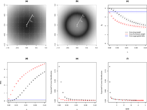
We construct masked data $\{Y_{1\lambda}(s_{i}),X_{1\lambda}(s_{i})\}$ by using equation (2.1) with both the Euclidean kernel weight $W^{\ast}_{\lambda}$ and the ring kernel weight $W_{1\lambda}$ which are defined as follows:

$$W^{\ast}_{\lambda}(u,s) = \exp(-\|s-u\|^{2}/\lambda),$$ (9)

$$W_{1\lambda}(u,s) = \exp(-|r^{2}_{s}-r^{2}_{u}|/\lambda).$$ (10)

The ring kernel weight $W_{1\lambda}(u,s)$ decreases exponentially as the difference between $r^{2}_{s}$ and $r^{2}_{u}$ increases, and such difference is positively associated with the difference between $X_{1}(s)$ and $X_{1}(u)$ according to the spatial pattern of the exposure. Figure 1(b) shows the contour plot of $W_{1\lambda}(s_{1},\cdot)$. On the other hand, the Euclidean kernel weight $W^{\ast}_{\lambda}(u,s)$ solely depends on $\|s-u\|$, the Euclidean distance between location $u$ and location $s$, and therefore does not account for prior knowledge on the spatial distribution of the exposure.

3.4 Example II

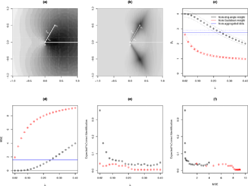
We assume that the exposure is eradiated from a point source $A$ and toward a certain direction. Specifically, we define $X_{2}(s)=7\times\break\exp(-r^{2}_{s}/6-\cos\theta_{s}/3)$ for $s\in[-1,1]\times[-1,1]$, where $\theta_{s}$ is the angle between the direction from point source $A$ to location $s$ and the direction that the exposure is toward, and $r_{s}$ is defined the same as in Example I. Figure 2(a) shows the contour plot of $X_{2}(s)$. The individual-level outcome is simulated from $Y_{2}(s_{i})\stackrel{{\scriptstyle\mathrm{i.i.d.}}}{{\sim}}\operatorname{Poisson}(e^{-36+4X_{2}(s_{i})})$. Aggregated data of exposure and outcome are constructed by calculating group summaries of $\{Y_{2}(s_{i}),X_{2}(s_{i})\}$ as described in Section 3.1.

We construct masked data $\{Y_{2\lambda}(s_{i}),X_{2\lambda}(s_{i})\}$ by using equation (2.1) with the Euclidean kernel weight (9) and the ring angle kernel weight

$$W_{2\lambda}(u,s)=\exp\bigl{(}-(|r^{2}_{s}-r^{2}_{u}|+2|\cos\theta_{s}-\cos\theta_{u}|)/\lambda\bigr{)},$$

which decreases exponentially as the difference between $r^{2}_{s}$ and $r^{2}_{u}$ increases as well as the difference between $\cos\theta_{s}$ and $\cos\theta_{u}$ increases. Figure 2(b) shows the contour plot of $W_{2\lambda}(s_{1},\cdot)$.

Figure 2: Example II of spatially varying exposure, weight function for spatial smoothing, estimates, and disclosure risk. (a) Contour plot of exposure from point source A toward a certain direction: $X_{2}(s)=7\exp(-r^{2}_{s}/6-\cos\theta_{s}/3)$, with cells for spatial aggregation. (b) Contour plot of ring angle weight function $W_{2\lambda}(s_{1},s)=\exp(-(|r^{2}_{s}-r^{2}_{s_{1}}|+2|\cos\theta_{s}-\cos\theta_{s_{1}}|)/\lambda)$ for calculating spatially smoothed exposure and outcome data at location $s_{1}$, from individual-level exposure $X_{2}(s)$ in (a) and individual-level outcome $Y_{2}(s)$ simulated by $Y_{2}(s)\sim\operatorname{Poisson}(\exp(-36+\beta X_{2}(s)))$ where $\beta=4$, with $\lambda=0.5$. (c) Estimates of $\beta_{\lambda}$ with “naive” 95$\%$ confidence intervals by fitting model $Y_{2\lambda}(s)\sim\operatorname{Poisson}(\exp(\mu_{\lambda}+\beta_{\lambda}X_{2\lambda}(s)))$ where $\{Y_{2\lambda}(s),X_{2\lambda}(s)\}$ are constructed using the ring angle weight function in (b) and using the Euclidean weight function $W^{\ast}_{\lambda}(s_{1},s)=\exp(-\|s-s_{1}\|^{2}/\lambda)$, with reference lines at $\beta=4$ and at the estimate from aggregated data. (d) Mean square error (MSE) of $\beta_{\lambda}$ using “naive” variance. (e) Identification disclosure risk measured by the expect percentage of correct record matching. (f) Disclosure risk versus MSE for utility-risk trade-off.

3.5 Example III

We assume that the exposure is eradiated from a point source $A$ but blocked in a certain area, such as blocked by a mountain, so the blocked area receives no exposure. Specifically, we define the unblocked area to be $s_{x}\leq 0.4$ or $\cos\vartheta_{s}\leq 0.625$ for $s\in[-1,1]\times[-1,1]$, where $s_{x}$ is the $x$-axis value of location $s$ and $\vartheta_{s}$ is the angle between the positive $x$-axis and the direction from point source $A$ to location $s$. We define the exposure $X_{3}(s)=7\exp(-r^{2}_{s}/2.5)\cdot I_{s}$ for $s\in[-1,1]\times[-1,1]$, where $I_{s}$ is the indicator that $s$ is located within the unblocked area, and $r_{s}$ is defined the same as in Examples I and II. Figure 3(a) shows the contour plot of $X_{3}(s)$. The individual-level outcome is simulated from $Y_{3}(s_{i})\stackrel{{\scriptstyle\mathrm{i.i.d.}}}{{\sim}}\operatorname{Poisson}(e^{-24+4X_{3}(s_{i})})$. Aggregated data of exposure and outcome are constructed by calculating group summaries of $\{Y_{3}(s_{i}),X_{3}(s_{i})\}$ as described in Section 3.1.

Figure 3: Example III of spatially varying exposure, weight function for spatial smoothing, estimates, and disclosure risk. (a) Contour plot of exposure from point source A but blocked in certain area: $X_{3}(s)=7\exp(-r^{2}_{s}/2.5)\cdot I_{s}$ where $I_{s}$ is the indicator of location $s$ in the unblocked area, with cells for spatial aggregation. (b) Contour plot of ring block weight function $W_{3\lambda}(s_{1},s)=\exp(-|r^{2}_{s}-r^{2}_{s_{1}}|/\lambda)\cdot(I_{s}=I_{s_{1}})$ for calculating spatially smoothed exposure and outcome data at location $s_{1}$, from individual-level exposure $X_{3}(s)$ in (a) and individual-level outcome $Y_{3}(s)$ simulated by $Y_{3}(s)\sim\operatorname{Poisson}(\exp(-24+\beta X_{3}(s)))$ where $\beta=4$, with $\lambda=0.5$. (c) Estimates of $\beta_{\lambda}$ with “naive” 95$\%$ confidence intervals by fitting model $Y_{3\lambda}(s)\sim\operatorname{Poisson}(\exp(\mu_{\lambda}+\beta_{\lambda}X_{3\lambda}(s)))$ where $\{Y_{3\lambda}(s),X_{3\lambda}(s)\}$ are constructed using the ring block weight function in (b) and using the Euclidean weight function $W^{\ast}_{\lambda}(s_{1},s)=\exp(-\|s-s_{1}\|^{2}/\lambda)$, with reference lines at $\beta=4$ and at the estimate from aggregated data. (d) Mean square error (MSE) of $\beta_{\lambda}$ using “naive” variance. (e) Identification disclosure risk measured by the expect percentage of correct record matching. (f) Disclosure risk versus MSE for utility-risk trade-off.

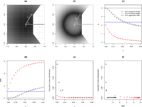
We construct masked data $\{Y_{3\lambda}(s_{i}),X_{3\lambda}(s_{i})\}$ by using equation (2.1) with the Euclidean kernel weight (9) and the ring block kernel weight

$$W_{3\lambda}(u,s)=\exp(-|r^{2}_{s}-r^{2}_{u}|/\lambda)\cdot(I_{s}=I_{u}),$$

which assigns nonzero weight only when location $u$ and location $s$ are both in the blocked or unblocked area. In addition, the nonzero weight from $W_{3\lambda}(u,s)$ decreases exponentially as the difference between $r^{2}_{s}$ and $r^{2}_{u}$ increases. Figure 3(b) shows the contour plot of $W_{3\lambda}(s_{1},\cdot)$.

3.6 Results

Results of Example I on parameter estimates, MSE and identification risk averaged across the 500 simulation replicates are shown in Figure 1(c)–(e), respectively. Specifically, Figure 1(c) shows the estimated $\beta_{\lambda}$ as a function of $\lambda$ for the ring kernel weight (10) and the Euclidean kernel weight (9), with the “naive” 95$\%$ confidence intervals. By “naive” we mean that the confidence intervals are computed by fitting model (7) directly, and therefore do not account for the possible correlation between the masked data as pointed out earlier in Section 2.2. The reference lines are placed at the true value of $\beta$ and at the estimated $\beta_{e}$, from which the bias of estimating the exposure coefficient by using the estimated $\beta_{\lambda}$ can be evaluated. Figure 1(d) shows the MSE as a function of $\lambda$ for the two kernel weights, where in this example MSE is largely determined by the bias. The reference lines are placed at the MSE from regression using the original data (in which the bias part is 0) and the MSE of $\beta_{e}$. Figure 1(e) shows the identification disclosure risk of the masked data set measured by the expected percentage of correct record matching, as a function of $\lambda$ for the two kernel weights. Figure 1(f) plots the disclosure risk versus MSE, which shows the trade-off between data utility and disclosure risk.

We find that data masking using the ring kernel weight (10) leads to smaller bias and MSE when estimating the exposure coefficient than masking using the Euclidean kernel weight (9), for all $\lambda$ values that are considered. It suggests that when using the masked data for loglinear regression, a masking procedure that preserves the spatial pattern of the original individual-level exposure and outcome data can lead to better estimates in terms of smaller bias and MSE than a masking procedure that does not do so. As $\lambda$ increases, the bias and MSE increase for both kernel weights, while the differences in the bias and MSE between the two kernel weights decrease. This increase in the bias/MSE and decrease in the bias/MSE differences suggest that in the presence of a high degree of masking, choice for the form of masking may be less influential on the resultant bias/MSE. Moreover, comparing the estimated $\beta_{\lambda}$ and $\beta_{e}$, we find that for small values of $\lambda$, the bias and MSE is smaller when using the estimated $\beta_{\lambda}$ from the ring kernel weight (10).

On the other hand, we find that the disclosure risk is lower when using the Euclidean kernel weight (9) for data masking compared to using the ring kernel weight (10). This is not unexpected because masked data constructed using the ring kernel weight is more informative about the original true values. However, with a tolerable potential disclosure risk [$<$0.2 which is used as an example cutoff in Reiter (2005a)], masked data when constructed using the ring kernel weight can lead to better MSE which cannot be achieved by using the Euclidean kernel weight with a comparable $\lambda$. Same as the trend for bias and MSE, the differences in the disclosure risk between the two kernel weights become small as $\lambda$ increases.

Similar results of Example II and Example III are shown in Figure 2(c)–(f) and Figure 3(c)–(f).

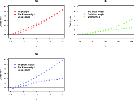
Figure 4 shows the width ratios comparing the 95% “naive” confidence intervals versus the percentile confidence intervals obtained from the empirical distribution of the estimates across the 500 simulations, for the estimates of $\beta_{\lambda}$ in the three examples respectively. Width ratio when $\lambda=0$ (the solid dot) is calculated using the nonsmoothed data, that is, the individual-level data. We find that in these three examples, the “naive” confidence intervals generally overestimate the uncertainty of the $\beta_{\lambda}$ estimates, and the degree of overestimation increases as $\lambda$ increases. In addition, for Examples II and III where the spatial patterns of exposure are nonisotropic, the degree of overestimation differs for the weight functions with and without accounting for prior knowledge on the spatial pattern of exposure.

Figure 4: Width ratios comparing the 95$\%$ “naive” confidence intervals (CI) versus the percentile CI obtained from the empirical distributions of the estimates across the 500 simulations, for the estimates of $\beta_{\lambda}$ in (a) Example I, (b) Example II, and (c) Example III of the simulation studies. Width ratio when $\lambda=0$ (the solid dot) is calculated using the nonsmoothed data.

4 Application to Medicare data

We apply our method to the study of racial disparities in risks of mortality for a sample of the U.S. Medicare population.

4.1 Data source

We extract a large data set at individual-level from the Medicare government database. Specifically, it includes individual age, race, gender and a day-specific death indicator over the period 1999–2002, for more than 4 million black and white Medicare enrollees who are 65 years and older residing in the Northeast region of the U.S. People who are younger than 65 at enrollment are eliminated because they are eligible for the Medicare program due to the presence of either a certain disability or End Stage Renal Disease and therefore do not represent the general Medicare population.

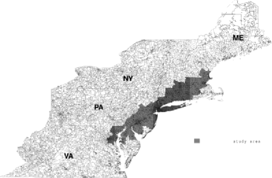
Figure 5 shows the study area which includes 2095 zip codes in 64 counties in the Northeast region of the U.S. We select the counties whose centroids are located within the range that covers the Northeast coast region of the U.S., and we exclude zip codes without available study population from the study map. This area covers several large, urban cities including Washington DC, Baltimore, Philadelphia, New York City, New Haven and Boston. It has the advantage of high population density and substantial racial diversity.

Figure 5: Location of the 2095 zip codes included in our study area.

We categorize the age of individuals into 5 intervals based on age in his/her first year of observation: [65, 70), [70, 75), [75, 80), [80, 85) and [85, $+$). This categorization facilitates detection of age effects because differences in the risks of mortality for one-year increase in age are relatively small. We “coarsen” the daily survival information into yearly survival indicators. By doing so, we define our outcome as the probability of the occurrence of death for an individual in one year. This definition adjusts for the differential follow-up time.

4.2 Statistical models and data masking

Let $i$ denote individual, $j$ denote zip code, $t$ denote year, and $D_{ijt}$ be the death indicator for individual $i$ in zip code $j$ in year $t$. Similarly as in Zhou, Dominici and Louis (2010a), we define the individual-level model as

$$\operatorname{\mathbf{logit}}\operatorname{Pr}(D_{tij}=1) = \beta_{0}+\beta_{1}\mathit{race}_{ij}+\mathit{age}_{ij}\bolds{\beta}_{2}$$

$${}+\beta_{3}\mathit{gender}_{ij}+(\mathit{age}\times\mathit{gender})_{ij}\bolds{\beta}_{4}.$$

Geographic locations for each individual are needed to spatially smooth the individual-level data. However, from the Medicare data we only have the longitude and latitude of the zip code centroids. Therefore, we apply a two-step masking procedure on the individual-level data, where we first aggregate the individual-level data to zip code-level, and we then spatially smooth the zip-code level aggregated data to construct the masked data at the zip code-level.

Specifically, let $D_{++j}$ denote the total death count and $n_{j}$ denote the total person-years of zip code $j$. We first obtain from aggregation $\{\%\ \mathit{black}_{j}$, $\%\ \mathit{agecat}_{j}$, $\%\ \mathit{male}_{j}$, $\%\ (\mathit{agecat}\times\mathit{male})_{j}$, $p_{j}=D_{++j}/n_{j}$, $j=1,\ldots,J\}$, which are the marginal distributions of race, age, gender, the joint distribution of age and gender, and the mortality rate, respectively, of each zip code.

Due to the complex spatial pattern of the zip code-level covariates, we use kernel smoothers with bivariate normal density kernel weights for spatial smoothing, so the shape of the smoothing weight is flexible by varying the correlation parameter value of the bivariate normal distribution. Let the vector $s=\{s_{1},s_{2}\}$ denote the location of a zip code, where $s_{1}$ and $s_{2}$ are the longitude and latitude of the zip code centroid, respectively. We use smoothing kernel weights of the general form

$$W_{\lambda}(u,s)=\exp\bigl{(}-(s_{1}-u_{1},s_{2}-u_{2})^{T}\Sigma^{-1}_{\lambda}(s_{1}-u_{1},s_{2}-u_{2})/2\bigr{)},$$

where

$$\Sigma_{\lambda}=\lambda\pmatrix{\sigma_{1}^{2}&\rho\sigma_{1}\sigma_{2}\vspace*{2pt}\cr\rho\sigma_{1}\sigma_{2}&\sigma_{2}^{2}},$$

$\sigma_{1}^{2}$ and $\sigma_{2}^{2}$ are the variances of the longitude and latitude data of the 2095 zip codes, respectively. We consider for $\rho$ the following three values:

1. $\rho=0$, so the weight solely depends on the Euclidean distance $\|s-u\|$;

2. $\rho=0.5$, so higher weight is assigned to $s$ in the northeast and southwest directions of $u$;

3. $\rho=-0.5$, so higher weight is assigned to $s$ in the northwest and southeast directions of $u$.

Let $p_{j\lambda}$ denote the smoothed mortality rate of zip code $j$ from which we calculate the smoothed death count $D_{++j\lambda}=p_{j\lambda}\cdot n_{j}$. Let $\%\ \mathit{black}_{j\lambda}$, $\%\ \mathit{agecat}_{j\lambda}$, $\%\ \mathit{male}_{j\lambda}$, $\%\ (\mathit{agecat}\times\mathit{male})_{j\lambda}$ denote the smoothed marginal distributions of race, age, gender and the smoothed joint distribution of age and gender, respectively, of zip code $j$. We specify the model for masked data as

$$D_{++j\lambda} \sim \operatorname{Bin}(n_{j},p_{j\lambda}),$$

$$\operatorname{logit}p_{j\lambda} = \beta_{0\lambda}+\beta_{1\lambda}\%\ \mathit{black}_{j\lambda}+\bolds{\beta}_{2\lambda}\%\ \mathit{agecat}_{j\lambda}$$

$${}+\beta_{3\lambda}\%\ \mathit{male}_{j\lambda}+\bolds{\beta}_{4\lambda}\%\ (\mathit{agecat}\times\mathit{male})_{j\lambda}.$$

The zip code-level nonsmoothed aggregated data are also used to fit model (4.2).

To evaluate the identification disclosure risk, we consider the scenario that a data intruder possesses correct zip code-level demographic data and seeks the matching with the masked zip code-level data set in order to obtain information on the zip code-level mortality. Specifically, the released data set consists of $\%\ \mathit{black}_{j\lambda}$, $\%\ \mathit{agecat}_{j\lambda}$, $\%\ \mathit{male}_{j\lambda}$ and $p_{j\lambda},j=1,\ldots,2095$, and the data intruder possess the correct $\%\ \mathit{black}_{j}$, $\%\ \mathit{agecat}_{j}$ and $\%\ \mathit{male}_{j}$.

4.3 Choice of association measure

The common approach to report the association between race and mortality risks is to report the race coefficients $\beta_{1}$ in model (4.2) and $\beta_{1\lambda}$ in model (4.2), whose interpretation is subjected to the coding of the race covariate. For direct understanding of the difference in the risk of death between the black and white populations, we define and report the population-level odds ratio (OR) of death comparing Blacks versus Whites, which is a function of the predicted values [Zhou, Dominici and Louis (2010a)]. Therefore, interpretation of this association measure does not depend on model parameterization (e.g., on covariate centering and scaling).

Specifically, let

$$P_{tijb} = \operatorname{Pr}(D_{tij}=1|\mathit{race}_{ij}=\mathit{Black},\mathit{age}_{ij},\mathit{gender}_{ij}),$$

$$P_{tijw} = \operatorname{Pr}(D_{tij}=1|\mathit{race}_{ij}=\mathit{White},\mathit{age}_{ij},\mathit{gender}_{ij})$$

denote the predicted probabilities of death in year $t$ for a black person and a white person, respectively, whose other covariates values are the same as the $i$th individual in the $j$th zip code. We define the population-level OR from the individual-level model (4.2) as follows:

$$\mathit{OR}=\frac{P_{\cdot\cdot\cdot b}Q_{\cdot\cdot\cdot w}}{P_{\cdot\cdot\cdot w}Q_{\cdot\cdot\cdot b}},$$

where

$$P_{\cdot\cdot\cdot b} = \sum_{t,i,j}P_{tijb},\qquad P_{\cdot\cdot\cdot w}=\sum_{t,i,j}P_{tijw},$$

$$Q_{\cdot\cdot\cdot b} = 1-P_{\cdot\cdot\cdot b},\qquad Q_{\cdot\cdot\cdot w}=1-P_{\cdot\cdot\cdot w}.$$

Similarly, we define population-level $\mathit{OR}_{\lambda}$ from model (4.2) using summary probabilities

$$P_{\cdot b\lambda}=\frac{\sum_{j}n_{j}P_{jb\lambda}}{\sum_{j}n_{j}}\quad\mbox{and}\quad P_{\cdot w\lambda}=\frac{\sum_{j}n_{j}P_{jw\lambda}}{\sum_{j}n_{j}},$$

where $P_{jb\lambda}$ and $P_{jw\lambda}$ are the predicted probabilities of death in one year for zip codes that consist of solely black and solely white populations, respectively, and whose marginal and joint distributions of age and gender are the same as zip code $j$. “Naive” standard errors of $\log\mathit{OR}_{\lambda}$ are calculated using the multivariate Delta Method [Casella and Berger (2002)]. In addition, bootstrap confidence intervals for $\log\mathit{OR}_{\lambda}$ are calculated using 1000 nonparametric bootstrap samples. Both “naive” and bootstrap confidence intervals for $\mathit{OR}_{\lambda}$ are obtained by exponentiating the corresponding confidence intervals for $\log\mathit{OR}_{\lambda}$.

4.4 Results

Figure 6(a)–(c) shows the estimates of $\mathit{OR}_{\lambda}$ under model (4.2) as a function of $\lambda$ for the three kernel weights respectively, with the 95% “naive” confidence intervals, confidence intervals using bootstrap standard error estimates and bootstrap percentile confidence intervals. $\mathit{OR}_{0}$ is estimated by fitting model (4.2) to the nonsmoothed zip code-level aggregated data. The reference line is placed at the estimate of OR under the individual-level model (4.2).

Figure 6: Estimates of $\mathit{OR}_{\lambda}$ under model (4.2) and identification disclosure risk as a function of $\lambda$ for the three weight functions. Estimates of $\mathit{OR}_{\lambda}$ is plotted with the 95$\%$ “naive” confidence intervals (CI), CI using bootstrap standard error (SE) estimates, and bootstrap percentile CI. $\mathit{OR}_{0}$ is estimated by fitting model (4.2) to the nonsmoothed zip code-level aggregated data. (a) Estimates of $\mathit{OR}_{\lambda}$ for bivariate normal density kernel weight with $\rho=0$. (b) Estimates of $\mathit{OR}_{\lambda}$ for bivariate normal density kernel weight with $\rho=0.5$. (c) Estimates of $\mathit{OR}_{\lambda}$ for bivariate normal density kernel weight with $\rho=-0.5$. (d) Identification disclosure risk measured by expected percentage of correct matching.

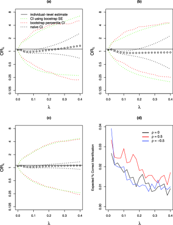
For small values of $\lambda$ ($<$0.1), the estimates of $\mathit{OR}_{\lambda}$ for all three kernel weights are smaller than the estimate of OR and therefore produce negative bias, while for larger values of $\lambda$ the bias differs substantially for different kernel weights. For example, data masking using the kernel weight with $\rho=0.5$ leads to consistent underestimation of the odds ratio for all $\lambda$ values that are considered. When using the kernel weight with $\rho=-0.5$ for data masking, the estimates of $\mathit{OR}_{\lambda}$ are less subject to bias than those from using the other two kernel weights. Differences in MSE between the three kernels can also be inferred from the plots, and we find that using the kernel weight with $\rho=-0.5$ leads to much smaller MSE than using the other two kernels. For all three kernel weights, the “naive” confidence intervals underestimate the uncertainty of the $\mathit{OR}_{\lambda}$ estimates, which is in the opposite direction of the relation between the “naive” and the appropriate confidence intervals in the simulation studies. The two bootstrap confidence intervals are wider than the “naive” confidence interval when $\lambda=0$, which suggests a systematic difference between the bootstrap confidence intervals and the “naive” confidence intervals regardless of smoothing. This systematic difference occurs because the nonsmoothed zip code-level aggregated data may not satisfy the Binomial model assumption in (4.2).

Figure 6(d) shows the identification disclosure risk of the masked data set as measured by the expected percentage of correct matches when using the three kernel weights for masking, as a function of $\lambda$. The disclosure risk for all three kernel weights are small, ranging from 0.01–0.04. The risk is similar for the masked data sets when using the kernel weight with $\rho=0$ and $\rho=-0.5$ for masking, and the risk when $\rho=0.5$ is slightly higher.

5 Discussion

We propose a special case of matrix masking based on spatial smoothing techniques, where the smoothing weight function controls the form of masking, and the smoothness parameter value directly measures the degree of masking. Therefore, data utility and disclosure risk can be calculated as functions of both the form and the degree of masking. In fact, the smoothing weight function $W$ can be any weight function and is not restricted by existing smoothing methods. With the variety of combinations of weight functions and smoothness parameter values, it is feasible to construct masked data that maintain high data utility while preserving confidentiality.

We consider a subclass of linear smoothers that produces masked data as weighted averages of the original data. Therefore, the masked data values are within a reasonable range. More importantly, correlation among the variables is invariant under linear transformation, which may intrinsically contribute to better data utility of the masked data. On the other hand, this subclass is a large class. It includes many commonly used smoothers. We do not expect major restriction by focusing on this subclass of linear smoothers.

Using our method, we investigate the utility of the masked data in terms of bias, variance and MSE of parameter estimates when using the masked data for loglinear and logistic regression analysis. Note that similar studies can be applied to any GLM. In addition, we evaluate the identification disclosure risk of the masked data set by calculating the expected percentage of correct record matching. In the simulation studies, we provide guidance for constructing masked data that can lead to better regression parameter estimates in terms of smaller bias and MSE for loglinear models, and we show the trade-off between better estimates and lower disclosure risk. Specifically, masked data can be constructed by using a smoothing weight function that accounts for prior knowledge on the spatial pattern of individual-level exposure, together with a reasonably low degree of masking. We provide guidance for how to select such a smoothing weight function for loglinear models. In addition, we provide candidate weight functions for three simplified but representative spatial patterns of exposure.

As is expected, masked data that can lead to better estimates are generally more informative about the original data values and therefore are subject to relatively higher identification disclosure risk. However, the flexibility in our data masking method enables constructing the masked data that can lead to good parameter estimates, while the disclosure risk is controlled at a low level. In the meanwhile, caution should be placed to the institute in releasing detailed information on the data masking approach along with masked data. It is pointed out in Section 2.1 that simultaneously releasing the smoothing weight function $W$ and the smoothness parameter $\lambda$ in the existence of $\mathcal{A}_{\lambda}^{-1}$ can lead to reidentification of original data. However, even if only partial information is released, for example, only the information that data are masked using smoothing and the smoothing weight function is released while the smoothing parameter value is not released, it is possible that a smart data intruder can still reconstruct the transformation matrix $\mathcal{A}_{\lambda}$.

We apply our data masking method to the study of racial disparities in risks of mortality for the Medicare population, and show how the bias and the variance of the estimated OR of death comparing blacks to whites, and how the identification disclosure risk, vary with the form and the degree of masking. The results suggest that in the absence of clear guidance, it is helpful to explore a large flexible family such as the bivariate normal density kernel to identify a weight function that can lead to both good utility and low identification risk for the masked data.

We compare the “naive” confidence intervals with the appropriate ones which account for the possible correlation among masked data in both the simulation studies and the data application, where we observe opposite directions in the relation between the “naive” and the appropriate confidence intervals. It suggests no general direction for that relation. One possible reason, which is also pointed out in Section 4.4, is that the unmasked data in the simulation study are simulated from Poisson distributions, while the unmasked data in the data application are real data and do not strictly follow the assumed binomial distribution. Therefore, in the data application, the standard errors account for both the correlation among the masked data and the discrepancy of the original data distribution from binomial.

The simulation study and data application results show that masked data constructed using our method can well preserve confidentiality. Specifically, the identification disclosure risk is reasonably low for all scenarios that we consider. Note that our calculation of the disclosure risk is conservative: we assume that an intruder possesses true values for all the regressors, and we use probability 1 for the component $\operatorname{Pr}(\mathbf{z}_{\lambda,1},\ldots,\mathbf{z}_{\lambda,j-1},\mathbf{z}_{\lambda,j+1},\ldots,\mathbf{z}_{\lambda,N}|\mathbf{z}_{\lambda,j},\break J=j,\mathbf{t})$ in the calculation. In addition, the flexibility in the selection of smoothing weight function $W$ and smoothness parameter $\lambda$ can also help control disclosure risk in addition to improving data utility.

Based on our method, we additionally derive a closed-form expression for first-order bias of the parameter estimates obtained using the masked data, for GLM that belong to the exponential family. The first-order bias calculation is not necessary when both individual-level exposure and health outcome data are available so the actual bias can be computed. It may be used by researchers who have only the individual-level exposure information to explore the possible bias in their analysis using masked data.

Although our proposed method uses spatial smoothing and therefore applies to spatial data, it can be easily generalized to other data types because the masking procedure is a smoothing technique that takes weighted averages of the original data. For example, the proposed method can be generalized to smoothing time series data by using the smoothing weight function $W_{\lambda}(\mu,s)$, where $\mu$ and $s$ denote time points. Also, note that an alternative method to mask spatial data is to mask the individual spatial location [see Armstrong, Rushton and Zimmerman (1999); Wieland et al. (1998)].

Appendix: First-order bias

We derive a closed-form expression for the first-order bias of estimating the regression coefficients in a GLM that belongs to the exponential family, when using data masked by our method. Let $\bolds{\beta}$ denote the vector of regression coefficients of a model specified for the original individual-level data. When the model belongs to the exponential family, its log likelihood can be expressed as

$$\operatorname{LL}(\bolds{\beta})=\sum_{i=1}^{N}\frac{Y_{i}\mathbf{X}_{i}\bolds{\beta}-b(\mathbf{X}_{i}\bolds{\beta})}{a(\phi)}+C(Y_{i},\phi),$$

$b^{\prime}(\mathbf{X}_{i}\bolds{\beta})=g^{-1}(\mathbf{X}_{i}\bolds{\beta})$, where $b^{\prime}(\cdot)$ is the derivative of function $b(\cdot)$, and $g(\cdot)$ is the link function. Substituting the individual-level data $\{Y_{i},\mathbf{X}_{i}\}$ by the masked data $\{Y_{\lambda}(s_{i}),\mathbf{X}_{\lambda}(s_{i})\}$, we obtain log likelihood of the analogous model when fitted to the masked data,

$$\qquad\operatorname{LL}_{\mathrm{m}}(\bolds{\beta}_{\lambda};\lambda) = \sum_{i=1}^{N}\frac{Y_{\lambda}(s_{i})\mathbf{X}_{\lambda}(s_{i})\bolds{\beta}_{\lambda}-b(\mathbf{X}_{\lambda}(s_{i})\bolds{\beta}_{\lambda})}{a_{\lambda}(\phi_{\lambda})}+C_{\lambda}(Y_{\lambda}(s_{i}),\phi_{\lambda}),$$ (13)

where $\bolds{\beta}_{\lambda}$ denotes the corresponding vector of regression coefficients. In order to calculate the MLE of $\bolds{\beta}_{\lambda}$, it is common procedure to calculate the score function from the likelihood (13) and take its expectation with respect to the “true” individual-level model $E\{Y_{i}|\mathbf{X}_{i}\}$. Denote the expected score function as $\overline{S}(\lambda,\bolds{\beta}_{\lambda})$ and denote $\bolds{\beta}(\lambda)$ as the solution s.t. $\overline{S}(\lambda,\bolds{\beta}(\lambda))=0$. It can be shown that $\bolds{\beta}(0)=\bolds{\beta}$. Taking the derivative of $\overline{S}(\lambda,\bolds{\beta}(\lambda))=0$ with respect to $\lambda$ and evaluating it at $\lambda=0$, we obtain the standard result:

$$\bolds{\beta}^{\prime}(0)=-(\overline{S}_{2}(0,\bolds{\beta}(0))^{-1}\cdot\overline{S}_{1}(0,\bolds{\beta}(0)),$$ (14)

where $\overline{S}_{1}$ and $\overline{S}_{2}$ are the partial derivatives with respect to the first and second components of $\partial\overline{S}/\partial\lambda$, respectively. Specifically,

$$\overline{S}_{1}(0,\bolds{\beta}(0)) = \sum_{i=1}^{N}\mathbf{X}_{i}^{T}\biggl{(}\int h(\mathbf{X}(s)\bolds{\beta})R_{0}(s_{i},s)\,dN(s)$$ (15)

$$\hskip 35.0pt{}-h^{\prime}(\mathbf{X}_{i}\bolds{\beta})\int\mathbf{X}(s)^{T}R_{0}(s_{i},s)\,dN(s)\cdot\bolds{\beta}\biggr{)}$$

$$\overline{S}_{2}(0,\bolds{\beta}(0)) = -\sum_{i=1}^{N}~{}h^{\prime}(\mathbf{X}_{i}\bolds{\beta})\cdot\mathbf{X}_{i}^{T}\mathbf{X}_{i},$$

where $R_{0}(s_{i},s)=\frac{\partial(W_{\lambda}(s_{i},s)/\int W_{\lambda}(s_{i},s)\,dN(s))}{\partial\lambda}|_{\lambda=0}$ and $h(\cdot)=g^{-1}(\cdot)$, inverse of the link function of the GLM. In practice, $\overline{S}_{1}(0,\bolds{\beta}(0))$ in (15) is calculated by substituting the the integrals by summations over all locations where the original individual-level data are available.

The quantity $\bolds{\beta}^{\prime}(0)$ denotes the instant bias of estimating $\bolds{\beta}$ using masked data, when changing from no masking to a very low degree of masking. As expected, when (i) $\mathbf{X}(s)$ is constant across all locations in $\mathbf{s}$, or (ii) $g(\cdot)$ is a linear function, $\overline{S}_{1}(0,\bolds{\beta}(0))$ is calculated to be 0, and therefore $\bolds{\beta}^{\prime}(0)=0$.

Using $\bolds{\beta}^{\prime}(0)$, we can approximate the bias of estimating $\bolds{\beta}$ when fitting a GLM using masked data whose degree of masking is $\lambda$, by calculating

$$\bolds{\beta}(\lambda)-\bolds{\beta}\approx\bolds{\beta}^{\prime}(0)\cdot\lambda.$$

This bias calculation can be extended to any function of $\bolds{\beta}$, for example, the predicted value. Specifically, bias in estimating $f(\bolds{\beta})$ can be approximated by

$$f(\bolds{\beta}(\lambda))-f(\bolds{\beta})\approx f^{\prime}(\bolds{\beta})\cdot\bigl{(}\bolds{\beta}(\lambda)-\bolds{\beta}\bigr{)}\approx f^{\prime}(\bolds{\beta})\cdot\bolds{\beta}^{\prime}(0)\cdot\lambda.$$

It can be seen that the first-order bias approximation can be easily generalized to approximation using higher-order terms of the Taylor series expansion in addition to the first-order term. Specifically,

$$\bolds{\beta}(\lambda)-\bolds{\beta} \approx \bolds{\beta}^{\prime}(0)\cdot\lambda+\bolds{\beta}^{\prime\prime}(0)\cdot\lambda^{2}/2+\cdots$$

$${}+\bolds{\beta}^{(n)}(0)\cdot\lambda^{n}/n!,\qquad n\geq 1.$$

Similarly, we can generalize the bias approximation of estimating $f(\bolds{\beta})$.

A limitation of the bias approximation using Taylor series expansion (Appendix: First-order bias) is that we ignore the remainder term $\bolds{\beta}^{(n+1)}(\xi)\cdot\frac{\lambda^{n+1}}{(n+1)!}$, $\xi\in(0,\lambda)$, which may not be small for large values of $\lambda$. Therefore, the approximation only captures the bias for $\lambda\approx 0$, that is, the instant direction and magnitude of the bias when changing from no masking to a very low degree of masking. It may not capture the total bias for a specified degree of masking. In the application of our method to the Medicare data, the first-order bias is calculated to be 0 for all three kernel weights because $R_{0}$ in (15) equals 0. In addition, when applying the bias approximation (Appendix: First-order bias) to the three examples in the simulation studies for $n=1,\ldots,5$, the bias approximation is calculated to be 0, while nonzero bias is shown by comparing the parameter estimates when using the masked data with the true parameter value.

References

- Armstrong, Rushton and Zimmerman (1999) Armstrong, M. P., Rushton, G. and Zimmerman, D. L. (1999). Geographically masking health data to preserve confidentiality. Stat. Med. 18 497–525.
- Bowman and Azzalini (1997) Bowman, A. W. and Azzalini, A. (1997). Applied Smoothing Techniques for Data Analysis: The Kernel Approach with S–Plus Illustrations. Oxford Univ. Press, Oxford.
- Casella and Berger (2002) Casella, G. and Berger, R. L. (2002). Statistical Inference. Duxbury Press, North Scituate, MA.
- Cox (1994) Cox, L. H. (1994). Matrix masking methods for disclosure limitation in microdata. Survey Methodology 20 165–169.
- Cox (1995) Cox, L. H. (1995). Network models for complementary cell suppression. J. Amer. Statist. Assoc. 90 1453–1462.
- Dalenius and Reiss (1982) Dalenius, T. and Reiss, S. P. (1982). Data-swapping: A technique for disclosure control. J. Statist. Plann. Inference 6 73–85. \MR0653248
- Dobra, Fienberg and Trottini (2003) Dobra, A., Fienberg, S. E. and Trottini, M. (2003). Assessing the risk of disclosure of confidential categorical data. In Bayesian Statistics 7, Proceedings of the Seventh Valencia International Meeting on Bayesian Statistics (J. Bernardo et al., eds) 125–144. Oxford Univ. Press, Oxford. \MR2003170
- Dobra et al. (2002) Dobra, A., Karr, A., Sanil, A. and Fienberg, S. (2002). Software systems for tabular data releases. Internat. J. Uncertain. Fuzziness Knowledge-Based Systems 10 529–544.
- Duncan and Lambert (1986) Duncan, G. T. and Lambert, D. (1986). Disclosure-limited data dissemination. J. Amer. Statist. Assoc. 81 10–28.
- Duncan and Pearson (1991) Duncan, G. T. and Pearson, R. W. (1991). Rejoinder: “Enhancing access to microdata while protecting confidentiality: Prospects for the future.” Statist. Sci. 6 237–239.
- Efron (1979) Efron, B. (1979). Bootstrap methods: Another look at the jackknife. Ann. Statist. 7 1–26. \MR0515681
- Efron and Tibshirani (1993) Efron, B. and Tibshirani, R. (1993). An Introduction to the Bootstrap. Chapman & Hall, New York. \MR1270903
- Fienberg (1994) Fienberg, S. E. (1994). Conflicts between the needs for access to statistical information and demands for confidentiality. Journal of Official Statistics 10 115–132.
- Fienberg, Makov and Steele (1998) Fienberg, S. E., Makov, U. E. and Steele, R. J. (1998). Disclosure limitation using perturbation and related methods for categorical data (with discussion). Journal of Official Statistics 14 485–511.
- Fienberg and McIntyre (2005) Fienberg, S. E. and McIntyre, J. (2005). Data swapping: Variations on a theme by Dalenius and Reiss. Journal of Official Statistics 21 309–323.
- Fienberg and Slavkovic (2004) Fienberg, S. E. and Slavkovic, A. B. (2004). Making the release of confidential data from multi-way tables count. Chance 17 5–10. \MR2061930
- Fienberg and Willenborg (1998) Fienberg, S. E. and Willenborg, L. C. R. J. (1998). Introduction to the special issue: Disclosure limitation methods for protecting the confidentiality of statistical data. Journal of Official Statistics 14 337–345.
- Fuller (1993) Fuller, W. A. (1993). Masking procedures for microdata disclosure limitation (with discussion). Journal of Official Statistics 9 383–406, 455–474.
- Gomatam, Karr and Sanil (2005) Gomatam, S., Karr, A. F. and Sanil, A. P. (2005). Data swapping as a decision problem. Journal of Official Statistics 21 635–655.
- Hastie, Tibshirani and Friedman (2001) Hastie, T., Tibshirani, R. and Friedman, J. H. (2001). The Elements of Statistical Learning: Data Mining, Inference, and Prediction: With 200 Full-Color Illustrations. Springer, New York. \MR1851606
- Karr et al. (2006) Karr, A. F., Kohnen, C. N., Oganian, A., Reiter, J. P. and Sanil, A. P. (2006). A framework for evaluating the utility of data altered to protect confidentiality. Amer. Statist. 60 224–232. \MR2246755
- Kim (1986) Kim, J. (1986). A method for limiting disclosure in microdata based on random noise and transformation. In American Statistical Association, Proceedings of the Section on Survey Research Methods 370–374. Amer. Statist. Assoc., Alexandria, VA.
- Raghunathan, Reiter and Rubin (2003) Raghunathan, T. E., Reiter, J. P. and Rubin, D. B. (2003). Multiple imputation for statistical disclosure limitation. Journal of Official Statistics 19 1–16.
- Reiter (2003) Reiter, J. P. (2003). Inference for partially synthetic, public use microdata sets. Survey Methodology 29 181–188.
- Reiter (2005a) Reiter, J. P. (2005a). Estimating risks of identification disclosure in microdata. J. Amer. Statist. Assoc. 100 1103–1112. \MR2236926
- Reiter (2005b) Reiter, J. P. (2005b). Releasing multiply imputed, synthetic public use microdata: An illustration and empirical study. J. Roy. Statist. Soc. Ser. A 168 185–205. \MR2113234
- Rubin (1993) Rubin, D. B. (1993). Comment on “Statistical disclosure limitation.” Journal of Official Statistics 9 461–468.
- Ruppert, Wand and Carroll (2003) Ruppert, D., Wand, M. and Carroll, R. (2003). Semiparametric Regression. Cambridge Series in Statistical and Probabilistic Mathematics 12. Cambridge Univ. Press, Cambridge. \MR1998720
- Simonoff (1996) Simonoff, J. S. (1996). Smoothing Methods in Statistics. Springer, New York. \MR1391963
- Slavkovic and Lee (2010) Slavkovic, A. and Lee, J. (2010). Synthetic two-way contingency tables that preserve conditional frequencies. Stat. Methodol. DOI: 10.1016/j.stamet.2009.11.002. To appear.
- Sullivan and Fuller (1989) Sullivan, G. and Fuller, W. A. (1989). The use of measurement error to avoid disclosure. In American Statistical Association, Proceedings of the Section on Survey Research Methods 802–807. Amer. Statist. Assoc., Alexandria, VA.
- Trottini and Fienberg (2002) Trottini, M. and Fienberg, S. E. (2002). Modelling user uncertainty for disclosure risk and data utility. Internat. J. Uncertain. Fuzziness Knowledge-Based Systems 10 511–528.
- Trottini et al. (2004) Trottini, M., Fienberg, S., Makov, U. E. and Meyer, M. (2004). Additive noise and multiplicative bias as disclosure limitation techniques for continuous microdata: A simulation study. Journal of Computational Methods for Science and Engineering 4 5–16.
- Wieland et al. (1998) Wieland, S. C., Cassa, C. A., Mandl, K. D. and Berger, B. (1998). Revealing the spatial distribution of a disease while preserving privacy. Proc. Natl. Acad. Sci. USA 105 17608–17613.
- Willenborg and Waal (1996) Willenborg, L. C. R. J. and Waal, T. D. (1996). Statistical Disclosure Control in Practice. Lecture Notes in Statistics 111. Springer, New York.
- Willenborg and Waal (2001) Willenborg, L. C. R. J. and Waal, T. D. (2001). Elements of Statistical Disclosure Control. Springer, New York. \MR1866909
- Woo et al. (2009) Woo, M.-J., Reiter, J. P., Oganian, A. and Karr, A. F. (2009). Global measures of data utility for microdata masked for disclosure limitation. The Journal of Privacy and Confidentiality 1 111–124.
- Zhou, Dominici and Louis (2010a) Zhou, Y., Dominici, F. and Louis, T. A. (2010a). Racial disparities in risks of mortality in a sample of the U.S. medicare population. J. Roy. Statist. Soc. Ser. C 59 319–339.
- Zhou, Dominici and Louis (2010b) Zhou, Y., Dominici, F. and Louis, T. A. (2010b). Supplement to “A smoothing approach for masking spatial data.” DOI: 10.1214/09-AOAS325SUPP.