Variable selection and regression analysis for graph-structured covariates withan application to genomics

Abstract

Graphs and networks are common ways of depicting biological information. In biology, many different biological processes are represented by graphs, such as regulatory networks, metabolic pathways and protein–protein interaction networks. This kind of a priori use of graphs is a useful supplement to the standard numerical data such as microarray gene expression data. In this paper we consider the problem of regression analysis and variable selection when the covariates are linked on a graph. We study a graph-constrained regularization procedure and its theoretical properties for regression analysis to take into account the neighborhood information of the variables measured on a graph. This procedure involves a smoothness penalty on the coefficients that is defined as a quadratic form of the Laplacian matrix associated with the graph. We establish estimation and model selection consistency results and provide estimation bounds for both fixed and diverging numbers of parameters in regression models. We demonstrate by simulations and a real data set that the proposed procedure can lead to better variable selection and prediction than existing methods that ignore the graph information associated with the covariates.

T1Supported in part by NIH Grants CA127334 and ES009111.

and

1 Introduction

There has been a growing interest in penalized least squares problems via $L_{1}$ or other types of regularization, especially in high-dimensional settings. Important penalty functions that can lead to sparse variable selection in regression include Lasso [Tibshirani (1996)] and SCAD [Fan and Li (2001)]. In particular, Lasso has the crucial advantage of being a convex problem, which leads to efficient computational algorithms by coordinate descent [Efron et al. (2004); Friedman et al. (2007); Wu and Lange (2008)] and sparse solutions. Zou (2006) proposed a novel adaptive Lasso procedure and presented results on model selection consistency and oracle properties of the parameter estimates. Zhao and Yu (2006) presented the irrepresentable condition for model selection consistency of Lasso. Zhang and Huang (2006) studied the sparsity and bias of the Lasso selection in high-dimensional linear regression. Fan and Li (2001) and Huang and Xie (2007) established the asymptotic oracle properties of the SCAD-penalized least squares estimators when the number of covariates is fixed or increases with the sample sizes. These novel penalized estimation methods are quite effective in selecting relevant variables and in predicting future outcomes, especially in high-dimensional settings.

New estimation procedures have also been developed in recent years to account for certain structures of the explanatory variables. These include the group Lasso procedure [Yuan and Lin (2006)] when the explanatory variables are grouped or organized in a hierarchical manner, the elastic net (Enet) procedure [Zou and Hastie (2005)] that deals with groups of highly correlated variables, and the fused Lasso [Tibshirani et al. (2005)] that imposes the $L_{1}$ penalty on the absolute differences of the regression coefficients in order to account for some smoothness of the coefficients. Nardi and Rinaldo (2008) established the asymptotic properties of the group Lasso estimator for linear models. Jia and Yu (2008) provided conditions for model selection consistency of the elastic net when $p\gg n$. Zou and Zhang (2009) proposed an adaptive elastic net with a diverging number of parameters and established its oracle property. Among these procedures, the Enet regularization and the fused Lasso are particularly appropriate for the analysis of genomic data, where the former encourages a grouping effect and the latter often leads to smoothness of the coefficient profiles for ordered covariates.

Motivated by a genomic application in order to account for network information in the analysis of genomic data, Li and Li (2008) proposed a network-constrained regularization procedure for fitting linear regression models and for variable selection, where the predictors in the regression model are genomic data that are measured on the genetic networks, which we call the graph-structured covariates. In particular, we assume that the covariates in the regression model are values of the nodes on a graph, where a link between two nodes may indicate a functional relationship between two genes in a genetic network or physical neighborhood between two voxels on brain images. Since many biological networks are constructed using data from high-throughput experiments, often there is a probability associated with an edge to indicate the certainty of a link. Such an edge probability can be used as a weight in a undirected graph, in which case we have a weighted graph. This graph-constrained regularization procedure is similar in spirit to the fused Lasso [Tibshirani et al. (2005)], both of which try to smooth the regression coefficients in certain ways. However, the fused Lasso does not utilize prior graph information. Second, instead of using the $L_{2}$ norm on the differences of the coefficients of the linked variables, the fused Lasso uses the $L_{1}$ norm on the differences, which tends to lead to the same regression coefficients for linked variables. In this paper we consider the general problem of regression analysis when the explanatory variables are nodes on a graph and present a cyclical coordinate descent algorithm [Friedman et al. (2007)] to implement the network-constrained regularization procedure of Li and Li (2008). This algorithm provides new insight on how neighboring variables affect the coefficient estimate of a node. We also extend the procedure of Li and Li (2008) to account for the possibility of different signs of the regression coefficients for neighboring variables. In addition, we provide theoretical results of the estimates, including sign consistency and error bounds of the estimator and $L_{2}$ consistency.

This paper is organized as follows. In Section 2 we describe the problem of regression analysis with covariates measured on graphs. We then present a graph-constrained estimation (Grace) procedure in order to account for the graph structures in Section 2.1 and an efficient coordinate descent algorithm to implement the proposed regularization methods in Section 2.3. We present the estimation and model selection consistency results in Section 3. We provide Monte Carlo simulation results in Section 4 and results from the application to the analysis of a data set on the gene expression of brain aging in Section 5. Finally, we give a brief discussion of the methods and results.

2 Regression analysis for covariates measured on a graph

Consider a weighted graph $G=(V,E,W)$, where $V=\{1,\ldots,p\}$ is the set of vertices that correspond to the $p$ predictors, $E=\{u\sim v\}$ is the set of edges indicating that the predictors $u$ and $v$ are linked on the graph and there is an edge between $u$ and $v$, and $W$ is the set of weights of the edges, where $w(u,v)$ denotes the weight of edge $e=(u\sim v)$. In genomic studies, biological networks are often represented as graphs, an edge between $u$ and $v$ on the graph can indicate some functional relationship between them and the weight can be used to measure the uncertainty of the edge between two vertices, for example, indicating the probability of having an edge between two variables when the graph is constructed from data. For each given sample, we assume that we have numerical measurements on each of the vertices and these measurements are treated as explanatory variables in a regression analysis framework. For the $u$th node, let $x_{iu}$ be the numerical measurement of the $u$th vertex on the graph for the $i$th individual. Further, let $\mathrm{x}_{u}=(x_{1u},\ldots,x_{nu})^{T}$ be the measured values at the $u$th vertex for $n$ i.i.d. samples. Consider the problem of variable selection and estimation where we have design matrix $\mathrm{X}=(\mathrm{x}_{1},\mathrm{x}_{2},\ldots,\mathrm{x}_{p})\in\mathcal{R}^{n\times p}$ and response vector $\mathrm{y}=(y_{1},y_{2},\ldots,y_{n})^{T}\in\mathcal{R}^{n}$, and they follow a linear model

$$\textrm{y}=\textrm{X}\beta+\varepsilon,$$ (1)

where $\varepsilon=(\varepsilon_{1},\ldots,\varepsilon_{n})^{T}\sim N(0,\sigma^{2}I_{n})$ and $\beta=(\beta_{1},\ldots,\beta_{p})^{T}$. Throughout this paper we assume that the predictors and the response are centered so that

$$\sum_{i=1}^{n}y_{i}=0,\qquad\sum_{i=1}^{n}x_{ij}=0,\quad\mbox{and}\quad\frac{1}{n}\sum_{i=1}^{n}x_{ij}^{2}=1\qquad\mbox{for }j=1,\ldots,p.$$

In this paper we consider that the design matrix $\mathrm{X}$ is a deterministic matrix in the fixed design settings.

When $p$ is large, we assume that model (1) is “sparse,” that is, most of the true regression coefficients $\beta$ are exactly zero. Without loss of generality, we assume the first $q$ elements of vector $\beta$ are nonzeroes. Denote $\beta_{(1)}=(\beta_{1},\ldots,\beta_{q})^{T}$ and $\beta_{(2)}=(\beta_{q+1},\ldots,\beta_{p})^{T}$, then element-wise $\beta_{(1)}\neq 0$ and $\beta_{(2)}=0$. Now write $\mathrm{X}_{(1)}$ and $\mathrm{X}_{(2)}$ as the first $q$ and last $p-q$ columns of $\mathrm{X}$, respectively, and let $\mathrm{C}=\frac{1}{n}{\mathrm{X}}^{T}\mathrm{X}$, which can then be expressed in the following block-wise form:

$${\mathrm{C}}=\pmatrix{\mathrm{C}_{11}&\mathrm{C}_{12}\cr\mathrm{C}_{21}&\mathrm{C}_{22}}.$$

The goal of this paper is to develop a regularization procedure for selecting the true relevant variables. Different from the existing approaches, we particularly account for the fact that the explanatory variables are related on a graph. We make this more precise in the next section.

2.1 Graph-constrained regularization and variable selection

In order to account for the fact that the $p$ explanatory variables are measured on a graph, we first introduce the Laplacian matrix [Chung (1997)] associated with a graph. Let the degree of the vertex $v$ be $d_{v}=\sum_{u\sim v}{w(u,v)}$. We say $u$ is an isolated vertex if $d_{u}=0$. Let $w(u,u)=0$. Following Chung (1997), we define the Laplacian matrix $\mathrm{L}$ for graph $G$ with the $uv$th element defined by

$$\mathrm{L}(u,v)=\cases{1-w(u,u)/d_{u},&\quad\mbox{if} $u=v$ and $d_{u}\neq 0$,\cr-{w(u,v)/\sqrt{d_{u}d_{v}}},&\quad\mbox{if} $u$ and $v$ are adjacent,\cr 0,&\quad\mbox{otherwise}.}$$ (2)

It is easy to verify that this matrix is positive semi-definite with 0 as the smallest eigenvalue and 2 as the largest eigenvalue when all the weights are 1 [Chung (1997)]. To allow the matrix to change with $n$, we further express this matrix in block-wise form,

$$\mathrm{L}=\pmatrix{\mathrm{L}_{11}&\mathrm{L}_{12}\cr\mathrm{L}_{21}&\mathrm{L}_{22}},$$

where $\mathrm{L}_{11}$ corresponds to the $q$ nodes that are relevant to the response and $\mathrm{L}_{22}$ corresponds to the $p-q$ nodes that are not relevant.

The Laplacian matrix has the following interpretations. For a given vector $\beta$, the edge derivative of $\beta$ along the edge $e(u,v)$ at $u$ is defined as

$$\frac{\partial\beta}{\partial e}\bigg{|}_{u}=\sqrt{w(u,v)}\biggl{(}\frac{\beta_{u}}{\sqrt{d_{u}}}-\frac{\beta_{v}}{\sqrt{d_{v}}}\biggr{)},$$

and, therefore, the local variation of $\beta$ at $u$ can be measured by

$$\sqrt{\sum\biggl{(}\frac{\partial\beta}{\partial e}\bigg{|}_{u}\biggr{)}^{2}}.$$

The smoothness of vector $\beta$ with respect to the graph structure can be expressed as

$$\beta^{T}\mathrm{L}\beta=\sum_{u\sim v}\biggl{(}\frac{\beta_{u}}{\sqrt{d_{u}}}-\frac{\beta_{v}}{\sqrt{d_{v}}}\biggr{)}^{2}w(u,v).$$

This variation functional for vectors $\beta$ penalizes vectors that differ too much over nodes that are linked. It contains a scaling by $\sqrt{d_{u}}$. One intuitive reason for such a scaling is to allow a small number of nodes with large $d_{u}$ to have more extreme values of $\beta_{u}$ while the usually much greater number of nodes with small $d_{u}$ should not ordinarily allow to have very large $\beta_{u}$. This variation functional has been widely used in semi-supervised learning on graphs [Zhu (2005); Zhou et al. (2004)].

For many problems with covariates measured on a graph, we would expect that the neighboring variables are correlated and, therefore, the regression coefficients would show some smoothness. One way to account for such a dependence of the regression coefficients is to impose a Markov random field (MRF) prior to the collection of $\beta$ vectors. The MRF decomposes the joint prior distribution of the $\beta_{u}$’s into lower-dimensional distributions based on the graph-neighborhood structures. A common MRF model is the Gaussian MRF model that assumes that the joint distribution of $\beta$ is given by

$$f(\beta)\propto\exp\biggl{\{}-\frac{1}{2\sigma^{2}}\beta^{T}\mathrm{L}\beta\biggr{\}},$$

which is an improper density. Based on this Gaussian MRF prior assumption, Li and Li (2008) introduced the following graph-constrained estimation of the regression coefficients, denoted by $\hat{\beta}$,

$$\hat{\beta}=\operatorname{argmin}\limits_{\beta}Q(\beta,\lambda_{1},\lambda_{2}),$$ (3)

where

$$Q(\beta,\lambda_{1},\lambda_{2}) = \|\mathrm{y}-\mathrm{X}\beta\|^{2}_{2}+\lambda_{1}\|\beta\|_{1}+\lambda_{2}\beta^{T}\mathrm{L}\beta$$

$$= (\mathrm{y}-\mathrm{X}\beta)^{T}(\mathrm{y}-\mathrm{X}\beta)+\lambda_{1}\sum_{u}|\beta_{u}|$$

$${}+\lambda_{2}\sum_{u\sim v}\biggl{(}\frac{\beta_{u}}{\sqrt{d_{u}}}-\frac{\beta_{v}}{\sqrt{d_{v}}}\biggr{)}^{2}w(u,v),$$

where $\mathrm{L}$ is the Laplacian as defined in (2) and the tuning parameters $\lambda_{1},\lambda_{2}$ control the amount of regularization for sparsity and smoothness. For the special case when $\lambda_{2}=0$, the estimate reduces to the Lasso, and when $\mathrm{L}$ is the identity matrix, the estimate reduces to the elastic net estimates.

2.2 An adaptive graph-constrained regularization

The Grace procedure may not perform well when two variables that are linked on the graph have different signs in their regression coefficients, in which case the coefficients are not expected to be locally smooth. For example, for genetic networks, two genes might be negatively correlated with the phenotypes and are therefore expected to have different signs in their regression coefficients. In order to account for the sign differences, we can first perform a standard least square regression when $p<n$ or the elastic net regression when $p\geq n$ and denote the estimate as $\tilde{\beta}$. We can then modify the above objective function as

$$Q^{*}(\lambda_{1},\lambda_{2},\beta) = \|\mathrm{y}-\mathrm{X}\beta\|^{2}_{2}+\lambda_{1}\|\beta\|_{1}+\lambda_{2}\beta^{T}\mathrm{L}^{*}\beta,$$

$$= \|\mathrm{y}-\mathrm{X}\beta\|^{2}_{2}+\lambda_{1}\sum_{j=1}^{p}|\beta_{j}|$$

$${}+{\lambda_{2}\sum_{u\sim v}\biggl{(}\frac{\mathrm{sign}(\tilde{\beta}_{u})\beta_{u}}{\sqrt{d_{u}}}-\frac{\operatorname{sign}(\tilde{\beta}_{v})\beta_{v}}{\sqrt{d_{v}}}\biggr{)}^{2}w(u,v)},$$

where

$$\mathrm{L}^{*}(u,v)=\cases{1-w(u,u)/d_{u},&\quad\mbox{if} $u=v$ and $d_{u}\neq 0$,\cr-\operatorname{sign}(\tilde{\beta}_{u})\operatorname{sign}(\tilde{\beta}_{v}){w(u,v)/\sqrt{d_{u}d_{v}}},&\quad\mbox{if} $u$ and $v$ are adjacent,\cr 0,&\quad\mbox{otherwise}.}$$

Note that the $\mathrm{L}^{*}$ matrix is still positive semi-definite. We call the $\beta$ defined by

$$\hat{\beta}=\operatorname{argmin}\limits_{\beta}Q^{*}(\beta,\lambda_{1},\lambda_{2})$$ (4)

the adaptive Grace (aGrace).

2.3 A coordinate descent algorithm

Friedman et al. (2007) presented a coordinate descent algorithm for solving the Lasso and the Enet regularization. In this section we develop a similar algorithm for the proposed graph-constrained regularization. We only present the detailed algorithm for the optimization problem defined by equation (3). Similar algorithms can be developed by the aGrace defined by (4). If we let $\lambda=(\lambda_{1}+2\lambda_{2})/2n$ and $\alpha=\lambda_{1}/(\lambda_{1}+2\lambda_{2})$, the Grace can be written as

$$\hat{\beta}(\lambda,\alpha)=\operatorname{argmin}\limits_{\beta}\biggl{\{}R(\beta):=\frac{1}{2n}\|\mathrm{y}-\mathrm{X}\beta\|_{2}^{2}+\lambda P_{\alpha}(\beta)\biggr{\}},$$ (5)

where

$$P_{\alpha}(\beta):=(1-\alpha)\frac{1}{2}\beta^{T}\mathrm{L}\beta+\alpha\|\beta\|_{1}=(1-\alpha)\frac{1}{2}\sum_{u\sim v}\biggl{(}\frac{\beta_{u}}{\sqrt{d_{u}}}-\frac{\beta_{v}}{\sqrt{d_{v}}}\biggr{)}^{2}+\alpha\sum_{u=1}^{p}|\beta_{u}|$$

is the graph-constrained penalty function.

Given a covariate $\mathrm{x}_{u}$, suppose we have estimated $\tilde{\beta}_{v}$ for $v\neq u$, and we want to partially minimize the objective function with respect to $\beta_{u}$. We can rewrite the objective function in $(\ref{Network})$ as

$$R(\beta) = \frac{1}{2n}\sum_{i=1}\biggl{(}y_{i}-\sum_{v\neq u}x_{iv}\tilde{\beta}_{v}-x_{iu}\beta_{u}\biggr{)}^{2}+\lambda(1-\alpha)\frac{1}{2}\sum_{v\sim u}\biggl{(}\frac{\beta_{u}}{\sqrt{d_{u}}}-\frac{\tilde{\beta}_{v}}{\sqrt{d_{v}}}\biggr{)}^{2}$$

$${}+\lambda\alpha|\beta_{u}|+\lambda(1-\alpha)\frac{1}{2}\mathop{\sum_{w\sim v}}_{w,v\neq u}\biggl{(}\frac{\tilde{\beta}_{w}}{\sqrt{d_{w}}}-\frac{\tilde{\beta}_{v}}{\sqrt{d_{v}}}\biggr{)}^{2}+\lambda\alpha\sum_{w\neq u}|\tilde{\beta}_{w}|.$$

We would like to compute the gradient at $\beta_{u}$, which only exists when $\beta_{u}\neq 0$. We first consider the case that the covariate $u$ is connected to some other nodes (variables) on the network. If $\beta_{u}>0$, due to the standardization of the covariates, we can differentiate the objective function $R(\beta)$ with respect to $\beta_{u}$ as

$$\frac{\partial R}{\partial\beta_{u}} = -\biggl{[}\frac{1}{n}\sum_{i=1}x_{iu}\biggl{(}y_{i}-\sum_{v\neq u}x_{iv}\tilde{\beta}_{v}\biggr{)}+\lambda(1-\alpha)\sum_{v\sim u}\frac{\tilde{\beta}_{v}}{\sqrt{d_{u}d_{v}}}\biggr{]}$$

$${}+\lambda\alpha+[1+\lambda(1-\alpha)]\beta_{u}.$$

Similarly, we can get the corresponding expression when $\beta_{u}<0$. Following the calculus by Donoho and Johnstone (1994) and Friedman et al. (2007), we obtain the coordinate-wise update form for $\beta_{u}$ as

$$\qquad\tilde{\beta}_{u}\leftarrow\frac{S((1/n)\sum_{i=1}x_{iu}(y_{i}-\tilde{y}_{i}^{(u)})+\lambda(1-\alpha)\sum_{v\sim u}{(\tilde{\beta}_{v}/\sqrt{d_{u}d_{v}})},\lambda\alpha)}{1+\lambda(1-\alpha)},$$ (6)

where:

• [$\bullet$]

• $\tilde{y}_{i}^{(u)}=\sum_{v\neq u}x_{iv}\tilde{\beta}_{v}$ is the partial residual for fitting $\beta_{u}$, that is, the fitted value excluding the contribution from $x_{iu}$. Since the covariates are standardized, $\frac{1}{n}\sum_{i=1}x_{iu}(y_{i}-\sum_{v\neq u}x_{iv}\tilde{\beta}_{v})$ is the simple least-squares coefficient while fitting the partial residual to $x_{iu}$, $i=1,\ldots,n$.

• $S(z,\gamma)$ is the soft-thresholding operator with value

  $$\operatorname{sign}(z)(|z|-\gamma)_{+}=\cases{z-\gamma,&\quad\mbox{if} $z>0$ and $\gamma<|z|$,\cr z+\gamma,&\quad\mbox{if} $z<0$ and $\gamma<|z|$,\cr 0,&\quad\mbox{otherwise}.}$$

When covariate $u$ is not connected to other nodes on the network, that is, when it has no neighbors, the corresponding coordinate-wise updating formula becomes the Lasso updating formula, that is

$$\tilde{\beta}_{u}\leftarrow S\biggl{(}\frac{1}{n}\sum_{i=1}x_{iu}\bigl{(}y_{i}-\tilde{y}_{i}^{(u)}\bigr{)},\lambda\alpha\biggr{)}.$$ (7)

Comparing the two updated forms of (6) and $(\ref{unconnected})$, an intuitive explanation can be drawn to help to understand the effect of the graph-constraint penalty on the coefficients. For an isolated predictor, the graph penalty is vanished and, thus, we only apply a soft-thresholding for the Lasso penalty, while for a connected predictor, form $(\ref{connected})$ takes into account the graph-constraint to the penalty by adding the scaled summation of the coefficients of the neighboring covariates to the simple least-squares coefficient and applying a proportional shrinkage for the graph penalty.

Given $\alpha$, we can compute the solution path for a decreasing sequence of values for $\lambda$, starting from the smallest value $\lambda_{\mathrm{max}}$ for which there is no covariate selected, that is, $\hat{\beta}=0$. Similar to Friedman et al. (2007), we can set $\lambda_{\mathrm{max}}=\mathrm{max}_{l}|\langle x_{l},y\rangle|/n\alpha$, $\lambda_{\mathrm{min}}=\epsilon\lambda_{\mathrm{max}}$ and construct a sequence of $K$ values of $\lambda$ decreasing from $\lambda_{\mathrm{max}}$ to $\lambda_{\mathrm{min}}$ on the log scale. Typical values are $\epsilon=0.001$ and $K=100$. Cross-validation (CV) can be used to select the two tuning parameters $\alpha$ and $\lambda$.

3 Error bound and model selection consistency for fixed and diverging $p$

In this section we provide some theoretical results on the proposed Grace procedure, including the error bounds, $L_{2}$ consistency of Grace and the model selection consistency for both fixed and diverging $p$ when $p$ tends to infinity with the sample size $n$. Our theoretical development follows that of Zhao and Yu (2006), Jia and Yu (2008) and Zou and Zhang (2009) on sign consistency of Lasso and adaptive elastic net estimates. In our theoretical analysis, we assume the following regularity conditions throughout: [(A1)]

We use $\Lambda_{\mathrm{min}}(\mathrm{M})$ and $\Lambda_{\mathrm{max}}(\mathrm{M})$ to denote the minimum and maximum eigenvalues of a positive definite matrix $\mathrm{M}$, respectively. We further assume that $\mathrm{C}=\frac{1}{n}\mathrm{X}^{T}\mathrm{X}$ is positive definite and

$$b\leq\Lambda_{\mathrm{min}}(\mathrm{C})\leq\Lambda_{\mathrm{max}}(\mathrm{C})\leq B,$$

where $b$ and $B$ are two positive constants that do not depend on $n$.

$\frac{1}{n}\max_{1\leq i\leq n}\sum_{j=1}^{p}x_{ij}^{2}\rightarrow 0$, as $n\rightarrow\infty$.

These two conditions assume that the predictor matrix has a reasonably good behavior and were also assumed in Zhao and Yu (2006) and in Zou and Zhang (2009). Condition (A1) is also the condition (F) in Fan and Peng (2004) and condition (A2) ensures that the rows of the matrix $\mathrm{X}$ behave like a sample from a probability distribution in $\mathcal{R}^{p}$ [Portnoy (1984)]. These two conditions hold naturally if one assumes that $x_{i}$ are i.i.d. with finite second moments.

3.1 Error bound and $L_{2}$-consistency of Grace

We first provide the following nonasymptotic risk bound for the Grace of the regression coefficients defined by (2.1) for any $p$ and $n$:

Theorem 3.1

Given the data $(\mathrm{y},\mathrm{X})$, define the Grace as

$$\hat{\beta}(\lambda_{1},\lambda_{2})=\operatorname{argmin}\limits_{\beta}\{\|\mathrm{y}-\mathrm{X}\beta\|^{2}_{2}+\lambda_{1}\|\beta\|_{1}+\lambda_{2}\beta^{T}\mathrm{L}\beta\},$$

for nonnegative tuning parameters $\lambda_{1}$ and $\lambda_{2}$. Then under the regularity condition (A1), we have

$$E(\|\hat{\beta}(\lambda_{1},\lambda_{2})-\beta\|_{2}^{2})\leq\frac{4\lambda_{2}^{2}\Lambda_{\max}^{2}(\mathrm{L})\|\beta_{(1)}\|_{2}^{2}+4pnB\sigma^{2}+2\lambda_{1}^{2}p}{n^{2}\Lambda_{\min}^{2}(\mathrm{C}+(\lambda_{2}/n)\mathrm{L})}.$$ (8)

The proof of this theorem is given in Li and Li (2010). Note that this result is not asymptotic and holds for any $p$ and $q<p$. From this theorem, under the regularity assumption (A1) and the following further assumptions on $p$ and the tuning parameters $\lambda_{1},\lambda_{2}$: [(A.3)]

$\lim_{n\rightarrow\infty}\frac{p}{n}=0$,

$\lim_{n\rightarrow\infty}\frac{\lambda_{1}\sqrt{p}}{n}=0$,

$\lim_{n\rightarrow\infty}\frac{\lambda_{2}}{n}=0$ and $\lim_{n\rightarrow\infty}\frac{\lambda_{2}\|\beta_{(1)}\|_{2}}{n}=0$, we have

$$\|\hat{\beta}(\lambda_{1},\lambda_{2})-\beta\|_{2}^{2}\stackrel{{\scriptstyle P}}{{\longrightarrow}}0,$$

which implies that the Grace of $\beta$ is $L_{2}$ consistent. This result implies that the Grace procedure chooses the important variables with high probability and that falsely chosen variables by Grace have very small coefficients. The $L_{2}$ consistency result suggests that we may use some hard-thresholding procedure to further eliminate the variables with very small Grace coefficients. Alternatively, an interesting randomized selection procedure proposed by Bickel, Ritov and Tsybakov (2008) can be used to further eliminate the variables with small estimated Grace coefficients. Note that under the classical setting where $p$, $q$ and $\beta_{i}$ are all fixed as $n\rightarrow\infty$, the assumptions (A3)–(A5) hold when $\lambda_{i}/n\rightarrow\infty,i=1,2.$

3.2 Model selection consistency when $p$ is fixed

We next establish the results on model selection consistency for the standard case where $p$ and $q$ are fixed when $n\rightarrow\infty$. Following Zhao and Yu (2006), we define the Grace of $\beta$ to be sign consistent if there exists $\lambda_{1}$ and $\lambda_{2}$ as functions of $n$ such that

$$\lim_{n\rightarrow\infty}\operatorname{Pr}\bigl{(}\operatorname{sign}(\hat{\beta}(\lambda_{1},\lambda_{2}))=\operatorname{sign}(\beta)\bigr{)}=1.$$

To establish the sign consistency of the Grace, we first provide the following graph-constrained irrepresentable condition (GC-IC): there exists $\eta>0$ and $\lambda_{1}>0$, $\lambda_{2}>0$, such that

$$\biggl{|}\biggl{(}\mathrm{C}_{21}+\frac{\lambda_{2}}{n}\mathrm{L}_{21}\biggr{)}\biggl{(}\mathrm{C}_{11}+\frac{\lambda_{2}}{n}\mathrm{L}_{11}\biggr{)}^{-1}\biggl{[}\operatorname{sign}\bigl{(}\beta_{(1)}\bigr{)}+\frac{2\lambda_{2}}{\lambda_{1}}\mathrm{L}_{11}\beta_{(1)}\biggr{]}$$

$${}\qquad\quad\hskip 178.0pt-\frac{2\lambda_{2}}{\lambda_{1}}\mathrm{L}_{21}\beta_{(1)}\biggr{|}$$

$$\qquad\leq\mathbf{1}-\eta,$$

where $\mathbf{1}$ is a vector of 1s with length $p-q$ and the inequality holds element-wise. Further, we assume that $\mathrm{C}\rightarrow\mathrm{C}_{0}$, where $\mathrm{C}_{0}$ is positive definite. The GC-IC is a consequence of the Karush–Kuhn–Tucker (KKT) conditions for the following constrained optimization problem that corresponds to the penalized optimization problem of equation (5):

$$\hat{\beta}(\lambda,\alpha)=\operatorname{argmin}\limits_{\beta}\biggl{\{}\frac{1}{2n}\|\mathrm{y}-\mathrm{X}\beta\|_{2}^{2}\dvtx P_{\alpha}(\beta)\leq\lambda\biggr{\}}.$$

Theorem 3.2

For fixed $p,q$ and $\beta$, if $\mathrm{C}\rightarrow\mathrm{C}_{0}$, where $\mathrm{C}_{0}$ is positive definite and condition (A.2) holds, the graph-constrained estimate is sign consistent if and only if GC-IC (3.2) holds for $\lambda_{1},\lambda_{2}$ that satisfy $\lambda_{1}/\sqrt{n}\rightarrow\infty$ and $\lambda_{i}/n\rightarrow 0$, for $i=1,2$.

This theorem is a special case of Theorem 3.3 and its proof is similar to that of Zhao and Yu (2006) for Lasso estimates. We therefore omit its proof in this paper. Note that the required conditions on the sparsity tuning parameter $\lambda_{1}$ are the same as those for the Lasso [Zhao and Yu (2006)], for example, $\lambda_{1}=\sqrt{n}\log n$ is a suitable choice. This theorem indicates that under some restrictive conditions of the design matrix and the Laplacian matrix of the network, the sign consistency property holds for the graph-constrained regularization. To gain further insight into GC-IC, consider the special cases when $\lambda_{2}$ is preselected and fixed and when $\lambda_{1}$ goes to infinity, the GC-IC reverses back to the irrepresentable condition for the Lasso given in Zhao and Yu (2006) and the graph-constrained penalty function $\lambda_{1}\|\beta\|_{1}+\lambda_{2}\beta^{T}\mathrm{L}\beta=\lambda_{1}(\|\beta\|_{1}+\frac{\lambda_{2}}{\lambda_{1}}\beta^{T}\mathrm{L}\beta)$ is reduced to the Lasso penalty.

3.3 Model selection consistency when $p$ diverges

We now consider the model selection consistency of the graph-constrained regularization procedure under the settings when the number of covariates $p$ also goes to infinity as $n\rightarrow\infty$, in which case, the assumptions and the regularity conditions for Theorems 3.1 and 3.2 become inappropriate as $\mathrm{C}$ does not converge and $\beta$ may change as $n$ grows. The following theorem shows that for the general scalings when $p,q$ and $n$ all go to infinity, under some additional conditions between $p,q$ and $n$, GC-IC also guarantees that the Grace is sign consistent in selecting the true model.

Theorem 3.3

Suppose each column of $\mathrm{X}$ is normalized to the $L_{2}$-norm of $n$ and GC-IC (3.2) holds. Define $\rho:=\min|(\mathrm{C}_{11}+\frac{\lambda_{2}}{n}\mathrm{L}_{11})^{-1}(\mathrm{C}_{11}\beta_{(1)})|$ and $\mathrm{C}_{\min}=\Lambda_{\min}(\mathrm{C}_{11})$, where $\Lambda_{\min}(\cdot)$ denotes the minimal eigenvalue. Let $W_{\max}=\max_{u,v}\{w(u,v)\}$. If $\lambda_{1}$ and $\lambda_{2}$ are chosen such that: [(a)]

If $\mathrm{L}_{12}=0$,

$$\frac{\lambda_{1}^{2}}{n\log(p-q)}\rightarrow\infty,$$

or if $\mathrm{L}_{12}\neq 0$,

$$\frac{\lambda_{1}^{2}}{\log(p-q)(n+{\lambda_{2}^{2}W_{\max}^{2}/(n\mathrm{C}_{\min})})}\rightarrow\infty.$$

If $\frac{1}{\rho}\{\sqrt{\frac{\log q}{n\mathrm{C}_{\min}}}+\frac{\lambda_{1}}{n}\|(\mathrm{C}_{11}+\frac{\lambda_{2}}{n}\mathrm{L}_{11})^{-1}\operatorname{sign}(\beta_{(1)})\|_{\infty}\}\rightarrow 0$, then the Grace $\hat{\beta}(\lambda_{1},\lambda_{2})$ is sign consistent as $n\rightarrow\infty$.

A proof analogous to Jia and Yu (2008) can be found in Li and Li (2010). Theorem 3.3 gives a general sign consistency result for the Grace for general scalings of $p,q$ and $n$. If $\mathrm{C}_{\min}\geq\alpha$ for some $\alpha>0$ and $\rho\leq\rho_{0}$ for some $\rho_{0}>0$, it is easy to check that the conditions $\log q/n\rightarrow\infty$ and $\lambda_{1}\sqrt{q}/n\rightarrow 0$ guarantee that condition (b) in Theorem 3.3 holds. In the settings when $p$ and $q$ are fixed, if $\mathrm{C}_{11}$ converges to a nonnegative definite matrix $\mathrm{C}_{110}$, $\rho$ converges to a nonnegative number. In addition, it is easy to verify that the conditions in Theorem 3.2 guarantee that the conditions (a) and (b) in Theorem 3.3 hold.

4 Monte Carlo simulations

We conducted Monte Carlo simulations to evaluate the proposed Grace and aGrace procedures and to compare the performance of this procedure with Lasso and Enet in terms of prediction errors and identification of relevant variables. We simulated the graph to mimic gene regulation modules. We used genes and variables interchangeably in this section. We assumed that the graph consisted of 200 unconnected regulatory modules with 200 transcription factors (TFs) and each regulated 10 different genes for a total of 2200 variables. Among these modules and genes, we further assumed that four TFs and their 10 regulated genes (for a total of 44 variables) were associated with the response based on the following model:

$$Y=\sum_{u=1}^{44}\beta_{u}X_{u}+\epsilon.$$ (10)

We considered two different models. For the first model, we assumed that the coefficients in model (10) were specified as

$$\beta = \biggl{(}2,\underbrace{\frac{2}{\sqrt{10}},\ldots,\frac{2}{\sqrt{10}}}_{10},-2,\underbrace{\frac{-2}{\sqrt{10}},\ldots,\frac{-2}{\sqrt{10}}}_{10},4,$$

$${}\;\underbrace{\frac{4}{\sqrt{10}},\ldots,\frac{4}{\sqrt{10}}}_{10},-4,\underbrace{\frac{-4}{\sqrt{10}},\ldots,\frac{-4}{\sqrt{10}}}_{10},0,\ldots,0\biggr{)},$$

and the $\epsilon$ was random mean-zero normal error with variance $\sigma^{2}=\sum_{u}\beta_{u}^{2}/4$. For each TF, the $\mathrm{X}$ value was simulated from a $N(0,1)$ distribution, and conditional on the value of the TF, we simulated the expression levels of the genes that they regulated from a conditional normal distribution with correlations of 0.2, 0.5 and 0.9, respectively. We therefore had a total of 2200 variables and 44 of them were relevant. For the second model, we considered the case when the regulated genes had different signs in regression coefficients, where the regression coefficients in model (10) have the same absolute values as in Model 1, but for each simulated module, three out of the 10 genes regulated by the TF had different signs from the other 7 genes. The $\mathrm{X}$ values were generated in the same way as in previous simulations. In this model, genes that are regulated by the same transcription factor are assumed to have different regression coefficients.

For each model, our simulated data consisted of a training set, an independent validation set and an independent test set with a sample size of 200 for all three data sets. Models were fitted on training data only, and the validation data were used to select the tuning parameters. We computed the prediction mean-squared errors on the test data set. For each model, we repeated the simulations 100 times. Table 1 shows the prediction mean-square errors for several different procedures. For Model 1 when the neighboring genes have the same signs in regression coefficients, we observed that the Grace gave the smallest prediction errors for all four models with different correlations among the predictors. Both Grace and Enet performed better than Lasso in prediction. When the correlation is very high, the prediction errors of these procedures were comparable, however, Grace still gave the smallest prediction error among the procedures compared. When the signs of the regression coefficients were the same, aGrace was reduced to Grace and gave the same prediction results. For Model 2 when the neighboring variables have different signs of coefficients, aGrace adjusting for the signs of the regression coefficients gave the smallest prediction errors, further indicating the importance of adjusting for the signs in the regularization. In general, Grace gave similar prediction results as the Enet, except when the correlation between the transcription factors and their regulated genes was very high, in which case Enet resulted in a slightly smaller prediction error.

Table 1: Comparison of prediction mean-square errors (SE) using Grace, aGrace, Enet and Lasso for three different correlation structures of 0.2, 0.5 and 0.9 between the transcription factors and their regulated genes for each of the two models considered. The results are based on 100 replications

	Model 1 (Cor)			Model 2 (Cor)
Method	0.2	0.5	0.9	0.2	0.5	0.9
Grace	24.93	23.22	22.56	53.08	42.07	28.20
	(2.97)	(2.41)	(2.20)	(6.45)	(5.03)	(2.87)
aGrace	24.93	23.22	22.56	27.70	26.23	25.55
	(2.97)	(2.41)	(2.20)	(3.66)	(3.03)	(2.76)
Enet	51.33	37.37	25.82	56.18	45.65	27.33
	(6.65)	(4.69)	(2.67)	(7.22)	(5.81)	(2.72)
Lasso	53.41	40.30	27.82	57.62	47.65	29.23
	(6.68)	(4.94)	(2.98)	(7.01)	(5.53)	(2.78)

Figure 1: Comparison of ROCs for Grace, aGrace, Enet and Lasso for Model 1 [plots (a) and (b)] and Model 2 [plots (c) and (d)] and for correlations of 0.2 [plots (a) and (c)] and 0.9 [plots (b) and (d)]. The ROCs were calculated as a function of the sparsity parameter $\lambda_{1}$. For Grace, aGrace and Enet, the tuning parameter $\lambda_{2}$ was selected based on 5-fold CV.

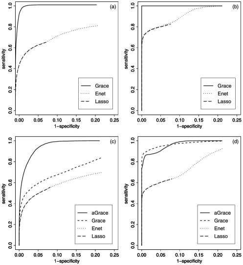
To compare the performance on variable selection, Figure 1 shows the receiver operating characteristic (ROC) curves of several different procedures in selecting the relevant variables for the models with correlation of 0.2 and 0.9 between the TF and their regulated genes. For Grace, aGrace and Enet, the ROC curves were obtained as a function of the sparsity parameter $\lambda_{1}$ with tuning parameter $\lambda_{2}$ selected based on 5-fold cross-validation among the values of 0.1, 1, 10, 100 and 1000. For Model 1 when the neighboring genes have the same signs in regression coefficients [Figure 1 plots (a) and (b)], Grace gave much larger areas under the ROC cruves than Enet and Lasso, indicating better performance in variable selection for Grace. In addition, five-fold cross-validation always chose the largest $\lambda_{2}=1000$ for Grace and $\lambda_{2}=0.1$ for Enet in all 100 replications. For Model 2 when the neighboring variables have different signs of coefficients, aGrace adjusting for the signs of the regression coefficients performed better than the other three procedures compared, resulting in larger areas under the curves, and Grace still performed better than Lasso and Enet on variable selections in both low and high correlation scenarios. When the correlation among the relevant variables is low, the 5-fold CV selected $\lambda_{2}=1000$ for aGrace and $\lambda_{2}=0.1$ for Enet in all 100 replications and selected $\lambda_{2}=100$ for Grace in most of the replications. When the correlation among the relevant variables was high, the 5-fold CV selected $\lambda_{2}=1000$ for aGrace and $\lambda_{2}=100$ for Grace in most of the 100 replications and selected $\lambda_{2}=0.1$ for Enet in all the replications.

5 Application to network-based analysis of gene expression data

To demonstrate the proposed method, we consider the problem of identifying age-dependent molecular modules based on the gene expression data measured in human brains of individuals of different ages published in Lu et al. (2004). In this study the gene expression levels in the postmortem human frontal cortex were measured using the Affymetrix arrays for 30 individuals ranging from 26 to 106 years of age. To identify the aging-regulated genes, Lu et al. (2004) performed simple linear regression analysis for each gene with age as a covariate. We analyzed this data set by combining the KEGG regulatory network information with the gene expression data [Kanehisa and Goto (2002)]. In particular, we limited our analysis to the genes that can be mapped to the KEGG regulatory work and focused on the problem of identifying the subnetworks of the KEGG regulatory network that are associated with human brain aging. By merging the gene expression data with the KEGG regulatory pathways, the final KEGG network includes 1305 genes and 5288 edges.

Table 2: Results of analysis of brain aging gene expression data by four different procedures, including the number of genes selected (No. genes), the number of linked KEGG edges (No. edges), the five-fold cross-validation error (CV error) and the values of the tuning parameters selected($\lambda_{2}$ for Grace, aGrace and Enet and $s_{1}=\sum_{v}|\beta_{v}|$)

	No. genes	No. edges	CV error	Tuning parameters
Grace	45	09	0.079	$\lambda_{2}=0.1$, $s_{1}=4.72$1
aGrace	73	28	0.077	$\lambda_{2}=0.01$, $s_{1}=6.97$
Enet	41	10	0.077	$\lambda_{2}=1.0$, $s_{1}=5.64$1
Lasso	18	00	0.098	$s_{1}=5.65$ $s_{1}=5.64$

We treated the logarithm of the individual age as the response variable and the expression levels (after $\log_{10}$ transformation) of 1305 genes on the KEGG network as the explanatory variables in our analysis. Table 2 shows the results of several different procedures where the tuning parameters were selected by five-fold cross-validations. Overall, we observed that the Lasso selected the fewest number of genes with relatively large cross-validation errors and Grace and Enet selected roughly the same number of genes with similar CV errors. However, the adaptive Grace resulted in more identified genes with similar CV errors than the other two procedures. Figure 2 shows the subnetworks identified by four different estimation procedures. As a comparison, we also included the genes selected by Lasso, although it did not select any linked pairs of genes on the KEGG network. It is interesting to note that as we impose more constraints on the regression coefficients, more linked genes are identified. Both Enet and Grace identified some common subnetworks that were associated with brain aging. These included fibroblast growth factors (FGF) and its receptors. It has been demonstrated that FGFs are associated with many developmental processes including neural induction [Bottcher and Niehrs (2005)] and are involved in multiple functions including cell proliferation, differentiation, survival and aging [Yeoh and de Haan (2007)]. It is also interesting to observe that mitogen-activated protein kinase (MAPK) (MAPK1 and MAPK9) and the specific MAPK kinase (MAP2K) were also identified by Enet and Grace. The MAPKs play important roles in induction of apoptosis [Hayesmoore et al. (2009)]. Other interesting genes include RAS protein-specific guanine nucleotide-releasing factor 1 (RASGRF1), the functionality of which is highly significant in various contexts of the central nervous system. In the hippocampus, RASGRF2 has been shown to interact with the NR2A subunits of NMDARs, triggering Ras-ERK activation and induction of long-term potentiation, a form of neuronal plasticity that contributes to memory storage in the brain [Tian et al. (2004); Lu et al. (2004)]. Finally, the insulin receptor gene (INSR) is also identified. INSR binds insulin (INS) and regulates energy metabolism. Evidence from model organisms, including results from fruit flies [Tatar et al. (2001)] and roundworms [Kimura et al. (1997)], relates INSR homologues to aging, most likely as part of the GH1/IGF1 axis. These results indicated that our method can indeed recover some biologically interesting molecular modules or KEGG subnetworks that are related to brain aging in humans.

Figure 2: Subnetworks identified by (a) Elastic net (Enet), (b) Grace and (c) aGrace for brain aging gene expression data (only those genes that are linked on the KEGG network are plotted).

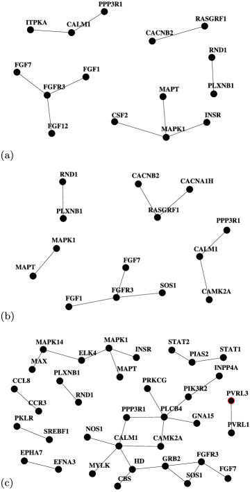
It is important to point out that the adaptive Grace identified several small sets of connected genes that were missed by Enet or the standard Grace. One of the subnetworks included EPHRIN and Eph receptor, both of which were found to be related to neural development and entohino-hippocampal axon targeting [Flanagan and Vaderhaeghen (1998); Stein et al. (1999)]. Another subnetwork was part of the Jak-State signaling, which is important in both mature and aging brains [De-Frajaa et al. (2000)]. Aging was also found to be associated with increased human T cell CC chemokine receptor gene expression [Yung et al. (2003)]. Other interesting subnetworks included PVRL3–PVRL1 that are associated with cell adhesion.

6 Discussion

We have introduced and studied the theoretical properties of a graph-constrained regularized estimation procedure for linear regressions in order to incorporate information coded in graphs. Such a regularization procedure can also be regarded as a penalized least squared estimation where the penalty is defined as a combination of the $L_{1}$ and $L_{2}$ penalties on degree-scaled differences of coefficients between variables linked on the graphs. This penalty function induces both sparsity and smoothness with respect to the graph structure of the regression coefficients. Simulation studies indicated that when the coefficients are similar for variables that are neighbors on the graph, the proposed procedure has better prediction and identification performance than other commonly used regularization procedures such as Lasso and elastic net regressions. Such improvement results from effectively utilizing the neighboring information in estimating the regression coefficients. If the smoothness assumption on the coefficients does not hold, we expect that the cross-validation selects a very small value of $\lambda_{2}$ and, therefore, the proposed procedure would perform similarly as the Lasso. In analysis of the brain aging gene expression data, different from Lasso, the new procedure tends to identify sets of linked genes on the networks, which often leads to better biological interpretation of the genes identified. Although the methods presented are largely motivated by applications in genomic data, they can be applied to other settings when the covariates are nodes on general graphs, such as in image analysis.

Although the methods presented in this paper were developed mainly for linear models, similar methods can be developed for the generalized linear models and the censored survival data regression models, where we can use the negative of the logarithm of the likelihood or partial likelihood as the loss function. Similar to the techniques presented in Friedman et al. (2007) and Wu and Lange (2008), we can use the coordinate descent procedure together with the iterative reweighted least square to obtain the solution path. Such models have great applications in genomic data analysis in identifying the genes or subnetworks that are associated with binary or censored survival data outcomes. Other extensions include replacing the $L_{1}$ part of the Grace penalty with other sparse penalty functions such as SCAD or bridge penalty [Huang et al. (2008)]. Important future research also includes how to handle covariates that are linked on directed graphs. Finally, to incorporate the fact that the linked nodes might be negatively correlated and the corresponding regression coefficients may have different signs, we introduced an adaptive sign-adjusted graph-constrained regularization procedure and showed that such a procedure can perform better than the original graph-constrained regularization. The theoretical property of such an adaptive procedure is unknown and is an area for future research.

References

- (1) Bickel, P. L., Ritov, Y. and Tsybakov, A. B. (2008). Hierarchical selection of variables in sparse high-dimensional regression. Technical report, Dept. Statistics, Univ. California, Berkeley.
- (2) Bottcher, R. T. and Niehrs, C. (2005). Fibroblast growth factor signaling during early vertebrate development. Endocrine Reviews 26 63–77.
- (3) Chung, F. (1997). Spectral Graph Theory. CBMS Reginal Conferences Series 92. Amer. Math. Soc., Providence, RI. \MR1421568
- (4) De-Fraja, C., Conti, L., Govoni, S., Battaini, F. and Cattaneo, E. (2000). STAT signalling in the mature and aging brain. International Journal of Developmental Neuroscience 18 439–446.
- (5) Donoho, D. and Johnstone, I. (1994). Ideal spatial adaptation via wavelet shrinkage. Biometrika 81 425–455. \MR1311089
- (6) Efron, B., Hastie, T., Johnstone, I. and Tibshirani, R. (2004). Least angle regression. Ann. Statist. 32 407–499. \MR2060166
- (7) Fan, J. and Li, R. (2001). Variable selection via nonconcave penalized likelihood and its oracle properties. J. Amer. Statist. Assoc. 96 1348–1360. \MR1946581
- (8) Fan, J. and Peng, H. (2004). Nonconcave penalized likelihood with a diverging number of parameters. Ann. Statist. 32 928–961. \MR2065194
- (9) Flanagan, J. G. and Vanderhaeghen, P. (1998). The ephrins and Eph receptors in neural development. Annual Review Neuroscience 21 309–345.
- (10) Friedman, J., Hastie, T., Hoefling, H. and Tibshirani, R. (2007). Pathwise coordinate optimization. Ann. Appl. Statist. 1 302–332. \MR2415737
- (11) Hayesmoore, J. B., Bray, N. J., Cross, W. C., Owen, M. J., O’Donovan, M. C. and Morris, H. R. (2009). The effect of age and the H1c MAPT haplotype on MAPT expression in human brain. Neurobiol. Aging 30 1652–1656.
- (12) Huang, J., Horowitz, J. L. and Ma, S. (2008). Asymptotic properties of bridge estimators in sparse high-dimensional regression models. Ann. Statist. 36 587–613.
- (13) Huang, J. and Xie, H. (2007). Asymptotic oracle properties of SCAD-penalized least squares estimators. In Asymptotics: Particles, Processes and Inverse Problems. IMS Lecture Notes Monogr. Ser. 55 149–166. IMS, Beachwood, OH. \MR2459937
- (14) Jia, J. and Yu, B. (2008). On model selection consistency of elastic net when . Technical Report 756, Dept. Statistics, Univ. California, Berkeley.
- (15) Kanehisa, M. and Goto, S. (2002). KEGG: Kyoto encyclopedia of genes and genomes. Nucleic Acids Research 28 27–30.
- (16) Kimura, K. D., Tissenbaum, H. A., Liu, Y. and Ruvkun, G. (1997). daf-2, an insulin receptor-like gene that regulates longevity and diapause in Caenorhabditis elegans. Science 277 942–946.
- (17) Li, C. and Li, H. (2008). Network-constrained regularization and variable selection for analysis of genomic data. Bioinformatics 24 1175–1182.
- (18) Li, C. and Li, H. (2010). Supplement to “Variable selection and regression analysis for graph-structured covariates with an application to genomics” DOI: 10.1214/10-AOAS332SUPP.
- (19) Lu, T., Pan, Y., Kao, S.-Y., Li, C., Kohane, I., Chan, J. and Yankner, B. A. (2004). Gene regulation and DNA damage in the aging human brain. Nature 429 883–891.
- (20) Nardi, Y. and Rinado, A. (2008). On the asymptotic properties of the group lasso estimator for linear models. Electron. J. Statist. 2 605–633. \MR2426104
- (21) Portnoy, S. (1984). Asymptotic behavior of M-estimators of regression parameters when is large. I. Consistency. Ann. Statist. 12 1298–1309. \MR0760690
- (22) Stein, E., Savaskan, N. E., Ninnemann, O., Nitsch, R., Zhou, R. and Skutella, T. (1999). A role for the Eph ligand ephrin-A3 in entorhino-hippocampal axon targeting. Journal of Neuroscience 19 8885–8893.
- (23) Tatar, M., Kopelman, A., Epstein, D., Tu, M. P., Yin, C. M. and Garofalo, R. S. (2001). A mutant Drosophila insulin receptor homolog that extends life-span and impairs neuroendocrine function. Science 292 107–110.
- (24) Tian, X., Gotoh, T., Tsuji, K., Lo, E. H., Huang, S. and Feig, L. A. (2004). Developmentally regulated role for Ras-GRFs in coupling NMDA glutamate receptors to Ras, Erk and CREB. EMBO J. 23 1567–1575.
- (25) Tibshirani, R. J. (1996). Regression shrinkage and selection via the lasso. J. Roy. Statist. Soc. Ser. B 58 267–288. \MR1379242
- (26) Tibshirani, R., Saunders, M., Rosset, S., Zhu, J. and Knight, K. (2005). Sparsity and smoothness via the fused lasso. J. Roy. Statist. Soc. Ser. B 67 91–108. \MR2136641
- (27) Wu, T. T. and Lange, K. (2008). Coordinate descent algorithms for lasso penalized regression. Ann. Appl. Statist. 2 224–244. \MR2415601
- (28) Yeoh, J. S. and de Haan, G. (2007). Fibroblast growth factors as regulators of stem cell self-renewal and aging. Mechanisms of Ageing and Development 128 17–24.
- (29) Yuan, M. and Lin, Y. (2006). Model selection and estimation in regression with grouped variables. J. Roy. Statist. Soc. Ser. B 68 49–67. \MR2212574
- (30) Yung, R. L. and Mo, R. (2003). Aging is associated with increased human T cell CC chemokine receptor gene expression. Journal of Interferon & Cytokine Research 23 575–582.
- (31) Zhang, C. and Huang, J. (2006). The sparsity and bias of the Lasso selection in high-dimensional linear regression. Ann. Statist. 36 1567–1594. \MR2435448
- (32) Zhao, P. and Yu, B. (2006). On model selection consistency of Lasso. J. Mach. Learn. Res. 7 2541–2567. \MR2274449
- (33) Zhou, D., Bousquet, O., Lal, T., Weston, J. and Scholkopf, B. (2004). Learning with local and global consistency. In NIPS 16 321–328. MIT Press, Cambridge, MA.
- (34) Zhu, X. (2005). Semi-supervised learning literature survey. Technical Report 1530, Computer Sciences, University of Wisconsin–Madison.
- (35) Zou, H. (2006). The adaptive lasso and its oracle properties. J. Amer. Statist. Assoc. 101 1418–1429. \MR2279469
- (36) Zou, H. and Hastie, T. (2005). Regularization and variable selection via the elastic net. J. Roy. Statist. Soc. Ser. B 67 301–320. \MR2137327
- (37) Zou, H. and Zhang, H. H. (2009). On the adaptive elastic net with a diverging number of parameters. Ann. Statist. 37 1733–1751. \MR2533470