Prediction-based classification for
longitudinal biomarkers

Abstract

Assessment of circulating CD4 count change over time in HIV-infected subjects on antiretroviral therapy (ART) is a central component of disease monitoring. The increasing number of HIV-infected subjects starting therapy and the limited capacity to support CD4 count testing within resource-limited settings have fueled interest in identifying correlates of CD4 count change such as total lymphocyte count, among others. The application of modeling techniques will be essential to this endeavor due to the typically nonlinear CD4 trajectory over time and the multiple input variables necessary for capturing CD4 variability. We propose a prediction-based classification approach that involves first stage modeling and subsequent classification based on clinically meaningful thresholds. This approach draws on existing analytical methods described in the receiver operating characteristic curve literature while presenting an extension for handling a continuous outcome. Application of this method to an independent test sample results in greater than $98\%$ positive predictive value for CD4 count change. The prediction algorithm is derived based on a cohort of $n=270$ HIV-1 infected individuals from the Royal Free Hospital, London who were followed for up to three years from initiation of ART. A test sample comprised of $n=72$ individuals from Philadelphia and followed for a similar length of time is used for validation. Results suggest that this approach may be a useful tool for prioritizing limited laboratory resources for CD4 testing after subjects start antiretroviral therapy.

Prediction-based classification for longitudinal biomarkers

T1Supported by the National Institutes of Health (R01-AI056983 to A. S. F., R01-AI51225 to L. J. M. and U01-AI051986 to L. J. M.), the Philadelphia Foundation and the Fund from the Commonwealth Universal Research Enhancement Program, Pennsylvania Department of Health.

, , ,
, ,
and

1 Introduction

Chronic HIV infection results in the progressive depletion of CD4$+$ T lymphocytes from both lymphoid tissues and peripheral blood. Thus, the monitoring of peripheral blood CD4 count is the standard used in decision-making concerning initiation of antiretroviral therapy (ART), as well as monitoring response to ART over time. In 2002 and again in 2006, the World Health Organization (WHO) proposed guidelines for administration of ARTs in an effort to provide a clear public health approach to utilization of these limited, yet very powerful drugs (WHO-Report, 2006). This series of recommendations includes routine collection and monitoring of CD4 counts to inform decisions regarding both initiation and switching of drug regimens. However, this report also acknowledges that collection of repeated CD4 counts may not be feasible in resource-limited settings due to the high costs associated with such monitoring. In these instances, clinicians are advised to initiate therapy in patients with asymptomatic HIV disease if total lymphocyte count (TLC) falls below 1200 cells$/$mm³.

In this manuscript we consider modeling strategies for using alternative surrogate markers within an acute window (3 years) post-initiation of therapy. Since publication of the WHO guidelines, several reports have been published on the clinical utility of alternative surrogate markers for monitoring post-therapy response and specifically the correlation between these markers and CD4 count [Bagchi et al. (2007); Bisson et al. (2006); Ferris et al. (2004); Mahajan et al. (2004); Kamya et al. (2004); Badri and Wood (2003); Bedell et al. (2003); Spacek et al. (2003); Kumarasamy et al. (2002)]. These investigations involve both cross-sectional and longitudinal data and implement a variety of straightforward analytical methods. Typically, cross-sectional comparisons between CD4 count and TLC as well as longitudinal comparisons between the change in each of these variables over a specified time period are performed using correlation analysis [Badri and Wood (2003); Kamya et al. (2004); Kumarasamy et al. (2002); Spacek et al. (2003)]. A summary of analytic strategies described for these settings, and their potential limitations, is given in the discussion; notably, the scientific findings of these reports are variable.

In this manuscript we describe a prediction-based classification (PBC) framework for predicting biomarker trajectories based on a binary decision rule. PBC was originally described in the setting of classifying HIV genetic variants that capture variability in a cross-sectional response to ART [Foulkes and DeGruttola (2002, 2003)]. Within this framework, we present two estimation procedures that both involve first stage modeling using a generalized linear mixed effect model (GLMM). In the first case, we dichotomize the biomarker a priori and use a logit link function. In this case, our approach reduces simply to fitting a logistic model coupled with a receiver operator characteristic (ROC) curve analysis, which is commonly applied in practice though it has not been described for this setting. The second estimation approach we present is based on fitting a linear mixed effects model to the observed CD4 count, as measured on a continuous scale. This later approach may offer improved predictive performance since it incorporates the full range of the continuous scale data. We describe both approaches further in Section 2. Section 3 then illustrates the method through application to two cohorts of HIV-1 infected individuals followed for three years after initiation of ART. Some simple extensions are described in Section 4 and finally we offer a discussion of how the approaches complement existing methods in Section 5.

2 Methods

Monitoring patient level CD4 counts over time may involve consideration of the observed counts at a given time point, the percent change in counts across a given period of time or some other function of patient level data. In general, interest lies in determining whether this function of the data is above or below a threshold value. For example, in monitoring absolute CD4 counts, thresholds of $200$ and $350$ are considered within well-established treatment administration guidelines. A threshold of $20\%$, on the other hand, is common for monitoring the percent change in CD4 between visits over time. We begin in this section by describing a general modeling framework. We then present an approach for predicting whether absolute CD4 is above a clinically meaningful threshold, at each of multiple discrete time points. In Section 4 we consider extensions of this framework that allow us to consider functions of the biomarker under study, such as percentage change over a given time period.

2.1 Generalized linear mixed effects model

Consider the generalized linear mixed effects model (GLMM) given by

$$g(E[\mathbf{Y}_{i}])=\mathbf{X}_{i}\beta+\mathbf{Z}_{i}b_{i},$$ (1)

where $\mathbf{Y}_{i}=(Y_{i1},\ldots,Y_{in_{i}})^{T}$ is a vector of the $n_{i}$ responses for individual $i$, $g(\cdot)$ is a link function, $\mathbf{X}_{i}$ is the $n_{i}\times M$ corresponding design matrix across $M$ covariates, $\beta$ is the fixed-effects parameter vector and $b_{i}\stackrel{{\scriptstyle\mathrm{i.i.d.}}}{{\sim}}\operatorname{MVN}(0,\mathbf{D})$. Here $\mathbf{Z}_{i}$ is the design matrix for the random effects and will typically include both an intercept and time component. One choice of $\mathbf{X}_{i}$ and $\mathbf{Z}_{i}$ is offered in the example of Section 3 and includes time varying values of white blood cell count and lymphocyte percentage. This model is a natural choice for this setting since repeated measures are taken over time on the same individual and the time points are unevenly spaced across individuals (Fitzmaurice, Laird and Ware, 2004).

In this manuscript we consider two approaches to fitting the model of equation (1). Since ultimately we are interested in predicting whether CD4 count is above (or below) a given threshold, we begin by modeling a dichotomized version of the observed CD4 data. We use the notation $Y_{ij}^{+}$ to indicate this binary representation of the observed data. That is, we define the dependent variable $Y_{ij}^{+}=I(\mathrm{CD4}_{ij}>K)$, where $\mathrm{CD4}_{ij}$ is the CD4 count at the $j$th time point for individual $i$ and $K$ is set equal to a clinically meaningful threshold. In this case, the canonical logit link is used to model the resulting binary outcome. Formally, if we let ${\theta}_{ij}=E[Y_{ij}^{+}]=\Pr(Y_{ij}^{+}=1)$, then equation (1) reduces in this setting to

$$\theta_{ij}=\frac{\exp[\mathbf{x}_{ij}\beta+\mathbf{z}_{ij}b_{i}]}{1+\exp[\mathbf{x}_{ij}\beta+\mathbf{z}_{ij}b_{i}]},$$ (2)

where $\mathbf{x}_{ij}$ and $\mathbf{z}_{ij}$ are the rows of $\mathbf{X}_{i}$ and $\mathbf{Z}_{i}$ respectively, corresponding to the $j$th measurement for individual $i$.

Second, we explore the utility of using the full range of the CD4 count data by modeling CD4 as a continuous variable. That is, we let $Y_{ij}=\mathrm{CD4}_{ij}$ and $g(\cdot)$ be the identity function, so that the model of equation (1) reduces to the linear mixed effects model (LMM), given by

$$Y_{ij}=\mathbf{x}_{ij}\beta+\mathbf{z}_{ij}b_{i}+\varepsilon_{ij},$$ (3)

where $\varepsilon_{ij}\sim N(0,\sigma^{2})$ and $b_{i}\perp\varepsilon_{ij}$. Since we ultimately aim to predict whether CD4 is above a given threshold, we then derive a prediction rule based on the estimated mean and variance components from this model.

2.2 Prediction-based classification

In fitting the mixed effects model of equation (1), we use the complete vector of observed data, given by $\mathbf{y}_{i}=(y_{i0},\ldots,y_{in_{i}})$, for all individuals in our learning sample. In general, we want to make predictions for new individuals under the assumption that only baseline values of $y_{i}$, given by $y_{i0}$, are observed. In the usual model fitting context, the predicted $y$ is generated using the empirical Bayes estimates of $b_{i}$, given by $\widehat{b}_{i}=E[b|\mathbf{y}_{i}]$. Notably, this conditions on this complete data vector and thus is not applicable to our setting, in which only the $y_{i0}$ are available. Thus, we need to arrive at an alternative estimate of the random effects that conditions only on the observed data for new individuals. We consider two approaches in the context of the linear mixed model. In the first case, we replace $\mathbf{y}_{i}$ with $\mathbf{X}_{i}\widehat{\beta}$ in the formula for $\widehat{b}_{i}$. This is our primary approach, described in Section 2.2.2 and applied in the example of Section 3. The second alternative we consider is to replace $\mathbf{y}_{i}$ with the baseline measure $y_{i0}$, which is presented as an extension in Section 4.

2.2.1 Binary outcome

After fitting the model of equation (1), mean and variance parameter estimates can be used to arrive at a predicted mean response for individual $i$ at the $j$th time point. Consider first the case in which we dichotomize CD4 count and fit the GLMM with a logit link, as described by equation (2). In this case, we have the predicted probability of CD4 count being above the threshold $K$ at the $j$th time point for individual $i$ given by

$$\widehat{\theta}_{ij}=\frac{\exp[\mathbf{x}_{ij}\widehat{\beta}+\mathbf{z}_{ij}\widehat{b}_{i}]}{1+\exp[\mathbf{x}_{ij}\widehat{\beta}+\mathbf{z}_{ij}\widehat{b}_{i}]},$$ (4)

where $\widehat{\beta}$ is a maximum likelihood estimate of $\beta$ and $\widehat{b}_{i}=E[b_{i}|\mathbf{y}_{i}^{+}]$ is the conditional mean of the random effects for individual $i$, given the observed data $\mathbf{y}_{i}^{+}$. Numerical integration techniques, such as Gaussian quadrature, are required for model fitting in this setting since no simple, closed-form solutions to maximum likelihood estimation are available.

=204pt $\bolds{y_{ij}^{+}}$ $\bolds{1}$ $\bolds{0}$ Total $\widehat{y}_{ij,\alpha}^{+}$ 1 $n_{11}$ $n_{12}$ $n_{1\cdot}$ 0 $n_{21}$ $n_{22}$ $n_{2\cdot}$ Total $n_{\cdot 1}$ $n_{\cdot 2}$ $n_{\cdot\cdot}$

Table 1: Contingency table notation for a given $\alpha$-prediction rule

A simple approach to prediction in this case is to let the predicted outcome, given by $\widehat{y}_{ij}$, equal $1$ if $\widehat{\theta}_{ij}\geq 0.50$ and $0$ otherwise, where $\widehat{\theta}_{ij}$ is defined by equation (4). Alternatively, we may want to choose a prediction rule that controls a clinically meaningful attribute. For example, in the CD4 prediction setting, we may want to control the false positive rate, defined as the proportion of individuals predicted to be above a safety threshold, when in fact their CD4 counts are below this safe limit. In this case, we define multiple rules, termed $\alpha$-prediction rules, that are given by

$$\widehat{y}_{ij,\alpha}^{+}=\cases{1,&\quad if ${\theta}_{ij}\geq 1-\alpha$,\cr 0,&\quad otherwise,}$$ (5)

where the unobserved $\theta_{ij}$ is replaced with the estimate $\widehat{\theta}_{ij}$. Notably, in making predictions for new individuals, the complete vector $\mathbf{y}^{+}$ is not available and, thus, $\widehat{b}_{i}=E[b_{i}|\mathbf{y}_{i}^{+}]$ in equation (4) cannot be calculated. In the example provided below, we let $\widehat{b}_{i}=E[b_{i}]=0$ for all $i$ in our test sample. An alternative approach for the linear model setting is described in Section 4.

Based on a given $\alpha$-prediction rule, we can generate the contingency table given in Table 1. Here the $n_{kl}$’s are the corresponding cell counts for $k,l=1,2$. For example, $n_{11}$ is the number of observations that are observed to be above the threshold ($y_{ij}^{+}=1$) and predicted to be above the threshold ($\widehat{y}_{ij,\alpha}^{+}=1$). The sensitivity of this rule is defined as the probability of correctly predicting an observation as being above the threshold among those responses that are in fact above the threshold and is given algebraically as $\Pr(\widehat{y}_{ij,\alpha}^{+}=1|y_{ij}^{+}=1)=n_{11}/n_{\cdot 1}$. The corresponding specificity is given by $\Pr(\widehat{y}_{ij,\alpha}^{+}=0|y_{ij}^{+}=0)=n_{22}/n_{\cdot 2}$ and the false positive rate is $\mathrm{FP}_{\alpha}=1-\mathrm{specificity}=n_{12}/n_{\cdot 2}$. Positive predictive value (PPV) and negative predictive value (NPV) are given by $(n_{11}/n_{1\cdot})$ and $(n_{22}/n_{2\cdot})$, respectively. By varying the value of $\alpha$ in equation (5), we generate multiple prediction rules and can construct a corresponding receiver operator characteristic (ROC) curve, which offers a visual representation of the trade-off between sensitivity and specificity. Specifically, an ROC curve is defined as a plot of the false positive rate ($x$-axis) and corresponding sensitivity ($y$-axis) for each of multiple classifiers, in our case prediction rules. In our setting, each $\alpha$-rule contributes one point to the ROC curve. We define the optimal rule as the one that controls the FP rate at a specified level, though alternative criterion are equally applicable.

Since the prediction rule given by equation (5) depends on an estimate of $\theta_{ij}$ that is derived based on the data, a cross-validation approach is necessary to obtain accurate estimates of predictive performance, including sensitivity and false positive rate. The motivation for this stems from the need to characterize the ability to make predictions on observations that did not contribute to the model fitting procedure. In this manuscript, we use an independent test sample to evaluate model performance. The approach proceeds as follows: First, model parameters are estimated using data arising from what we refer to as the learning sample. Second, the best $\alpha$-rule is identified based on the trade-off between sensitivity and specificity, again using the learning sample data. The estimates of predictive performance (e.g., false positive rate) based on the learning sample are referred to as resubstitution estimates as the data used for estimating error rates are the same as those used for deriving the prediction rule. Finally, measures of predictive performance for the chosen $\alpha$-rule are reported based on applying the rule to an independent data set, which we refer to as the test sample data. These test sample estimates are considered unbiased reflections of predictive performance, as independent data sets are used to generate the rule and describe its performance.

2.2.2 Continuous outcome

The prediction approach just described for a binary outcome involves simply fitting a logistic regression model and then generating an ROC curve based on several probability cutoffs. While, to our knowledge, this has not been applied to the setting of modeling biomarker trajectories over time and specifically to CD4 monitoring, similar approaches are used in practice in other settings [Tosteson et al. (1994); Tosteson and Begg (1988)]. One reason that this approach may not be optimal for the present setting is that CD4 count is measured on a continuous scale. We thus consider a simple extension of this approach that takes into consideration the full range of the observed CD4 count data. We begin by modeling $y_{ij}=\mathrm{CD4}_{ij}$ as a quantitative biomarker, using the linear mixed effects model of equation (3), and then derive a prediction approach similar to the one described by equation (5).

The model derived predicted value of $y_{ij}$ is given by $\widehat{y}_{ij}^{*}=\mathbf{x}_{ij}\widehat{\beta}+\mathbf{z}_{ij}\widehat{b}_{i}$. Here $\mathbf{x}_{ij}$ and $\mathbf{z}_{ij}$ are again respectively the rows of $\mathbf{X}_{i}$ and $\mathbf{Z}_{i}$ corresponding to the $j$th measurement for individual $i$, $\widehat{\beta}=\sum_{i=1}^{N}(\mathbf{X}_{i}^{T}\widehat{\Sigma}_{i}^{-1}\mathbf{X}_{i})^{-1}\mathbf{X}_{i}^{T}\widehat{\Sigma}_{i}\mathbf{y}_{i}$ is the least squares estimate of $\beta$, $\widehat{b}_{i}=E(b_{i}|\mathbf{y}_{i})=\widehat{\mathbf{D}}\mathbf{Z}_{i}^{T}\widehat{\Sigma}_{i}^{-1}(\mathbf{y}_{i}-\mathbf{X}_{i}\widehat{\beta})$ is the best linear unbiased predictor (BLUP) of the random effects for individual $i$, $\widehat{\Sigma}_{i}=\widehat{\operatorname{Var}}(\mathbf{y}_{i})=\mathbf{Z}_{i}\widehat{\mathbf{D}}\mathbf{Z}_{i}^{T}+\widehat{\sigma}^{2}I$, and $\widehat{\mathbf{D}}$ and $\widehat{\sigma}^{2}$ are the restricted maximum likelihood estimates of $\mathbf{D}$ and $\sigma^{2}$, respectively. Rather than estimate $\theta_{ij}=\Pr(\mathrm{CD4}_{ij}>K)$ of equation (5), we describe a one-sided prediction interval approach to identify a rule that is similar to the one described by this equation.

First note that the lower bound of the one-sided $(1-\alpha)$ prediction interval for $y_{ij}$ is given by

$$l_{ij,\alpha}=\widehat{y}_{ij}-z_{\alpha}\sqrt{\operatorname{Var}(\widehat{y}_{ij}-y_{ij})},$$ (6)

where $z_{\alpha}$ is the quantile of a standard normal corresponding to a $1-\alpha$ probability and $\operatorname{Var}(\widehat{y}_{ij}-y_{ij})$ is referred to as the prediction variance. In this manuscript, we treat this interval as an approximate credible interval, so that we are $(1-\alpha)\%$ certain that the random variable $Y_{ij}$ will be greater than this realization of the lower bound. In other words, $\Pr(Y_{ij}>l_{ij,\alpha})=(1-\alpha)\%$. Thus, if $l_{ij,\alpha}>K$, we are at least $(1-\alpha)\%$ certain that $Y_{ij}>K$. In other words, $l_{ij,\alpha}>K$ is equivalent to $\theta\geq(1-\alpha)$. As a result, the rule given by

$$\widehat{y}_{ij,\alpha}^{+}=\cases{1,&\quad if $l_{ij,\alpha}>K$,\cr 0,&\quad otherwise,}$$ (7)

is equivalent to the one given by equation (5). As described in McClean, Sanders and Stroup (1991) and McCulloch and Searle (2001), the prediction variance is given by $\operatorname{Var}(\widehat{y}_{ij}-\mathbf{x}_{ij}\beta-\mathbf{z}_{ij}b_{i})=\mathbf{x}_{ij}\operatorname{Var}(\widehat{\beta})\mathbf{x}_{ij}^{T}+\mathbf{z}_{ij}\operatorname{Var}(\widehat{b}_{i}-b_{i})\mathbf{z}_{ij}^{T}+\mathbf{x}_{ij}\operatorname{Cov}(\widehat{\beta},\widehat{b}_{i}-b_{i})\mathbf{z}_{ij}^{T}$ where $\operatorname{Var}(\widehat{\beta})=\sum_{i=1}^{N}(\mathbf{X}_{i}\Sigma_{i}^{-1}\mathbf{X}_{i}^{T})^{-1}$, $\operatorname{Var}(\widehat{b}_{i}-b_{i})=(\frac{1}{\sigma^{2}}\mathbf{Z}_{i}^{T}\mathbf{Z}_{i}+\mathbf{D}^{-1})^{-1}$ $-\operatorname{Cov}(\widehat{\beta},\widehat{b}_{i}-b_{i})\mathbf{X}_{i}^{T}\Sigma_{i}^{-1}\mathbf{Z}_{i}\mathbf{D}$ and $\operatorname{Cov}(\widehat{\beta},\widehat{b}_{i}-b_{i})=-\mathbf{D}\mathbf{Z}_{i}^{T}\Sigma_{i}^{-1}\mathbf{X}_{i}\operatorname{Var}(\widehat{\beta})$. In our setting, we are interested in the prediction variance for a new observed value and thus have an additional $\sigma^{2}$ term. That is, $\operatorname{Var}(\widehat{y}_{ij}-y_{ij})$ of equation (6) is equal to $\operatorname{Var}(\widehat{y}_{ij}-\mathbf{x}_{ij}\beta-\mathbf{z}_{ij}b_{i})+\sigma^{2}$. The appropriateness of treating the above prediction interval as a credible interval depends on prior assumptions about the parameters of our model. Since we are using this as a means of generating a prediction rule, and not as a tool for inference, this approximation seems reasonable. It also performs well in the example provided in Section 3. A study of the relative advantages of applying a fully Bayesian approach to approximating the posterior predictive distribution for this data setting is ongoing research.

Again a test sample is used to characterize model performance. In the linear mixed modeling setting, we note that $\operatorname{Var}(\widehat{\beta})$, $\widehat{\mathbf{D}}$ and $\widehat{\sigma}$ are estimated based on the model fitting procedure that uses the learning sample data. The remaining variance terms, $\operatorname{Var}(\widehat{b}_{i}-b_{i})$ and $\operatorname{Cov}(\widehat{\beta},\widehat{b}_{i}-b_{i})$ as well as the design elements $\mathbf{x}_{ij}$ and $\mathbf{z}_{ij}$ used in the calculation of $l_{ij,\alpha}$ of equation (6) are based on the test sample data. Notably, in both modeling frameworks, the BLUPs of the random effects can not be calculated for a new individual for whom the response $\mathbf{y}_{i}$ is not observed. One approach to handling this unobserved data is to replace $\mathbf{y}_{i}$ in the formula for $\widehat{b}_{i}$ with $\mathbf{X}_{i}\widehat{\beta}$ so that $\widehat{b}_{i}=\widehat{\mathbf{D}}\mathbf{Z}_{i}^{T}\widehat{\Sigma}_{i}^{-1}(\mathbf{X}_{i}\widehat{\beta}-\mathbf{X}_{i}\widehat{\beta})=0$. This results in reducing $\widehat{y}_{ij}$ to $\widehat{y}_{ij}=\mathbf{x}_{ij}\widehat{\beta}$ and is consistent with assigning each individual the estimated population average. In the example below, we use the prediction variance from the usual regression setting of $\operatorname{Var}(\widehat{y}_{ij}-y_{ij})=\mathbf{x}_{ij}\operatorname{Var}(\widehat{\beta})\mathbf{x}_{ij}^{T}+{\sigma}^{2}$. This prediction variance is less than the one described above; however, as we are varying $z_{\alpha}$ of equation (6) to generate a series of classification rules, the magnitude of the interval is less relevant. An alternative approach for handling the random effects in the linear mixed modeling framework is described in Section 4.

3 Example

The approach described in Section 2 is applied to a cohort of $N=270$ individuals from the Royal Free Hospital, London who were followed for up to three years after initiation of ART. Detailed information on the patient population and laboratory methods can be found in Smith et al. (2003, 2004). The aim of our analysis is to determine the utility of baseline CD4 count and repeated measures on WBC and lymphocyte percentage for predicting CD4 counts over time. Our approach uses the complete CD4 count data (across all time points) from a learning sample to generate a model; predictions based on this model are then made, for the resubstituted data as well as for an independent test sample, assuming that we only observe the baseline values of CD4. Consideration is given to two clinically meaningful CD4 count thresholds: $K=200$ and $K=350$ cells$/$mm³. All analyses are performed using R version 2.7.1. The median length of follow-up is $25$ months and the interquartile range (IQR) for length of follow-up is $(14,32)$ months. The median number of follow-up time points is $9$ with a full range of $2$ to $24$. In total, there are $2635$ records including baseline measurements. The median baseline CD4 count for this cohort is $219.5$ with an IQR equal to $(114,333)$.

Linear and generalized linear mixed effects models are fitted in R using the lme() and lmer() functions of the nlme and lme4 packages, respectively. We assume a piecewise linear mixed effects model for modeling CD4 count after initiation of ART (Fitzmaurice, Laird and Ware, 2004). This model is appropriate since CD4 count tends to rise rapidly for approximately one month and then proceeds to increase more gradually. Fixed effects for baseline CD4 count (on a log base 10 scale), baseline and time varying values of WBC and lymphocyte percentage and time before and after one month of follow-up are included in the model as predictors. In addition, interactions between each time component and baseline values of WBC and lymphocyte percent are included.

The design matrix $\mathbf{X}_{i}$ for the fixed effects of equation (1) is thus given by

$$\mathbf{X}_{i}=[\matrix{1_{N}&\mathbf{X}_{i1}&\mathbf{X}_{i2}}],$$

(8)

$$\eqntext{\mathbf{X}_{i1}=\left[\matrix{y_{i0}&w_{i0}&l_{i0}&t_{i1}&(t_{i1}-1)_{+}&w_{i1}&l_{i1}\cr y_{i0}&w_{i0}&l_{i0}&t_{i2}&(t_{i2}-1)_{+}&w_{i2}&l_{i2}\cr&&&\vdots&&&\cr y_{i0}&w_{i0}&l_{i0}&t_{in_{i}}&(t_{in_{i}}-1)_{+}&w_{in_{i}}&l_{in_{i}}}\right],\hskip 49.0pt}$$ (9)

$$\eqntext{\mathbf{X}_{i2}=\left[\matrix{t_{i1}*w_{i0}&t_{i1}*l_{i0}&(t_{i1}-1)_{+}*w_{i0}&(t_{i1}-1)_{+}*l_{i0}\cr t_{i2}*w_{i0}&t_{i2}*l_{i0}&(t_{i2}-1)_{+}*w_{i0}&(t_{i2}-1)_{+}*l_{i0}\cr&\vdots&&\cr t_{in_{i}}*w_{i0}&t_{in_{i}}*l_{i0}&(t_{in_{i}}-1)_{+}*w_{i0}&(t_{in_{i}}-1)_{+}*l_{i0}}\right],}$$ (10)

where $w_{i0}$ and $l_{i0}$ are respectively baseline WBC and baseline lymphocyte percent, $t_{ij}$ is time in months since initiation of ART, $(t_{ij}-1)_{+}$ is follow-up time after the first 1 month on ART for $t_{ij}>1$ and $0$ otherwise, and $w_{ij}$ and $l_{ij}$ are respectively WBC and lymphocyte percent at time $t_{ij}$. We define $y_{i0}$ in $\mathbf{X}_{i1}$ as $\log(\mathrm{CD4})$ for both the linear and generalized linear model although the response variable, given by $\mathbf{Y}_{i}=(Y_{i1},\ldots,Y_{in_{i}})$, is dichotomized for the generalized linear model setting. Notably, this model allows for two linear time trends, before and after 1 month of follow-up on ART. Random person specific intercepts and slopes before the knot are also assumed so that the design matrix $\mathbf{Z}_{i}$ for the random effects of equation (1) is given by

$$\mathbf{Z}_{i}=\left[\matrix{1&t_{i1}\cr 1&t_{i2}\cr&\vdots\cr 1&t_{in_{i}}}\right].$$ (11)

The random effects vector in equation (1) is given by $b_{i}^{T}=[\matrix{b_{i0}&b_{i1}}]$ representing the intercept and slope before the change point for individual $i$.

We begin by fitting the generalized linear model, as described in equation (2). In this case, post-baseline CD4 counts are dichotomized and used as the outcome in the model fitting procedure. Predicted probabilities of being above the CD4 threshold are estimated for each post-baseline time point for each individual. The results of applying a probability cutoff of $0.50$ are given in Table 2(a). We call this the “naive” approach since the cutoff does not incorporate information about the resulting prediction rule. While the sensitivities of these predictions rules ($0.98$ and $0.90$) are high for both thresholds, the corresponding false positive rates are also high ($0.54$ and $0.28$). This approach thus may not be appropriate for CD4 testing since it yields a high probability of falsely predicting that an individual’s CD4 count is within a safe limit.

Table 2: Observed and predicted counts (based on learning sample data)

(a) GLMM approach with a “naive” 0.50 probability cutoff Observed $\bolds{{>}200}$ $\bolds{{<}200}$ Total Predicted $>$200 $1932$ $215$ $2147$ $<$200 $\hphantom{00}34$ $184$ $218$ Total $1966$ $399$ $2365$ Observed $\bolds{{>}350}$ $\bolds{{<}350}$ Total Predicted $>$350 $1194$ $\hphantom{0}289$ $1483$ $<$350 $\hphantom{0}137$ $\hphantom{0}745$ $882$ Total $1331$ $1034$ $2365$

Table 2: Continued

(b) GLMM approach
			Observed				Observed
			$\bolds{{>}200}$	$\bolds{{<}200}$	Total		$\bolds{{>}200}$	$\bolds{{<}200}$	Total
Predictedtabl1	$>$200		$\hphantom{0}826$	$\hphantom{0}18$	$\hphantom{0}844$		1206	037	1243
	$<$200		$1140$	$381$	$1521$		0760	362	1122
	Total		$1966$	$399$	$2365$		1966	399	2365
			Observed				Observed
			$\bolds{{>}350}$	$\bolds{{<}350}$	Total		$\bolds{{>}350}$	$\bolds{{<}350}$	Total
Predictedtabl1	$>$350		$\hphantom{0}669$	$\hphantom{00}50$	$\hphantom{0}719$		0880	0103	983
	$<$350		$\hphantom{0}662$	$\hphantom{0}984$	$1646$		0451	0931	1382
	Total		$1331$	$1034$	$2365$		1331	1034	2365

(c) LMM approach
			Observed				Observed
			$\bolds{{>}200}$	$\bolds{{<}200}$	Total		$\bolds{{>}200}$	$\bolds{{<}200}$	Total
Predictedtabl1	$>$200		$1291$	$\hphantom{0}19$	$1319$		1558	038	1596
	$<$200		$\hphantom{0}675$	$380$	$1055$		0408	361	0769
	Total		$1966$	$399$	$2365$		1966	399	2365
			Observed				Observed
			$\bolds{{>}350}$	$\bolds{{<}350}$	Total		$\bolds{{>}350}$	$\bolds{{<}350}$	Total
Predictedtabl1	$>$350		$\hphantom{0}760$	$\hphantom{00}51$	$\hphantom{0}811$		0940	0103	1043
	$<$350		$\hphantom{0}571$	$\hphantom{0}983$	$1554$		0391	0931	1322
	Total		$1331$	$1034$	$2365$		1331	1034	2365

tabl1Predicted counts are based on rules with resubstitution FP rate estimates of approximately (but not greater than) $5\%$ (left panels) and $10\%$ (right panels).

Next, several $\alpha$ cutoffs are considered to generate multiple prediction rules and an ROC curve is generated, as illustrated in Figure 1(a). This is again based on the GLMM approach to model fitting. Data corresponding to rules with resubstitution FP rates of approximately (but not greater than) $5\%$ and $10\%$ and CD4 threshold cutoffs of $K=200$ and $350$ are provided in Tables 2(b) and (c). Resubstitution-based summary measures are given in Table 3(a). Based on a CD4 threshold of $K=200$, a FP rate of $0.09$ corresponds to a sensitivity of $0.61$, a positive predictive value of $0.97$ and a negative predictive value of $0.32$. For the same CD4 threshold, a FP of $0.05$ corresponds to a sensitivity of $0.42$, a positive predictive value of $0.98$ and a negative predictive value of $0.25$.

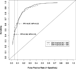
(a)

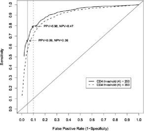
(b)

Figure 1: ROC curves based on resubstitution estimates. (a) GLMM, (b) LMM.

Table 3: Estimates of predictive performance

(a) GLMM approach
	GLMM (LS)				GLMM (TS)
	Sens	Spec	PPV	NPV	Sens	Spec	PPV	NPV
$K=200$:
$\mathrm{LS\ FP}<0.05$	0.42	0.95	0.98	0.25	0.66	0.96	0.99	0.31
$\mathrm{LS\ FP}<0.10$	0.61	0.91	0.97	0.32	0.77	0.96	0.99	0.39
$K=350$:
$\mathrm{LS\ FP}<0.05$	0.50	0.95	0.93	0.60	0.61	0.95	0.95	0.59
$\mathrm{LS\ FP}<0.10$	0.66	0.90	0.90	0.67	0.79	0.90	0.93	0.71

(b) LMM approach
	LMM (LS)				LMM (TS)
	Sens	Spec	PPV	NPV	Sens	Spec	PPV	NPV
$K=200$:
$\mathrm{LS\ FP}<0.05$	0.66	0.95	0.99	0.36	0.77	0.96	0.99	0.39
	(0.60, 0.75)		(0.98, 0.99)	(0.31, 0.46)
$\mathrm{LS\ FP}<0.10$	0.79	0.90	0.98	0.47	0.84	0.96	0.99	0.49
	(0.74, 0.83)		(0.97, 0.98)	(0.37, 0.54)
$K=350$:
$\mathrm{LS\ FP}<0.05$	0.57	0.95	0.94	0.63	0.73	0.93	0.95	0.67
	(0.44, 0.67)		(0.92, 0.95)	(0.56, 0.70)
$\mathrm{LS\ FP}<0.10$	0.71	0.90	0.90	0.70	0.84	0.90	0.94	0.77
	(0.65, 0.79)		(0.88, 0.92)	(0.66, 0.78)

Next we fitted the linear mixed effects model, as described by equation (3), to the observed CD4 count data. The resulting ROC curve illustrating the sensitivity and corresponding false positive rates in this cohort (resubstitution estimates) is given in Figure 1(b). Count data corresponding to rules for which thresholds are $K=200$ and $350$ and the resubstitution FP rates are approximately (but not greater than) $5\%$ and $10\%$ are given in Table 2(b). Corresponding summaries, as well as $95\%$ bootstrap confidence intervals (CIs), are reported in Table 3(b). To arrive at CIs, we repeatedly sample individuals with replacement and in each case, fit a linear mixed effects model. The prediction rule corresponding to FP rates of approximately (but not greater than) $5\%$ and $10\%$ are selected and corresponding resubstitution estimates of sensitivity, PPV and NPV are recorded. A total of $100$ bootstraps are performed for each threshold and the fifth and ninety-fifth percentiles reported.

Based on a CD4 cutoff of $200$, a FP rate of $0.10$ corresponds to a sensitivity of $0.79$ [$95\%$ CI (0.74, 0.83)]. In this case, the PPV is $0.98$ (0.97, 0.98) and the NPV is $0.47$ (0.37, 0.54). This corresponds to the rule in which $\alpha=0.035$. That is, an individual’s CD4 count is predicted to be above 200 if the probability that this measurement is greater than 200 is at least $1-0.035=96.5\%$. For the same CD4 threshold, a FP rate of $0.05$ corresponds to a sensitivity of $0.66$ (0.60, 0.75), PPV of $0.99$ (0.98, 0.99) and NPV of $0.36$ (0.31, 0.46).

In order to further evaluate model performance, we apply our prediction rule to $399$ observations across $n=72$ individuals from an independent cohort in Philadelphia. We use only baseline CD4 counts to make predictions, assuming that this is all that is available. The median baseline CD4 in this cohort is $260.5$ cells$/$mm³ and the IQR is $(159.0,354.2)$. Test sample estimates for sensitivity, false positive rate, PPV and NPV are provided in Tables 3(a) and (b) for each of the prediction rules. A tabular summary of counts for one rule based on the LMM approach is given in Table 4. The total count is $n=327$ since there are $399-72=327$ post-baseline measurements for this cohort. In this case, $n=240$ measurements are predicted to be above the threshold, while $87$ are predicted below. Since this is intended as a prioritization tool, this rule would suggest performing a true CD4 test on the $87$ observations that are predicted below the threshold to confirm the true value. A “savings” associated with this rule is $240/327=73\%$ since a CD4 test would not be required for this percentage of the observations. The “cost” is the associated false positive rate of $2/45=4.4\%$. Interestingly, the test sample estimates based on the LMM approach [Table 3(b)] appear slightly better than the resubstitution estimates. In fact, in some cases, these test sample estimates are greater than the $95\%$ bootstrap confidence limits derived based on the learning sample. This result may be a consequence of the overall slightly higher baseline CD4 count in the Philadelphia (test sample) cohort. A discussion of the potential utility of stratified analysis (e.g., according to baseline CD4 counts) is provided in Section 5.

=216pt Observed $\bolds{{>}200}$ $\bolds{{<}200}$ Total Predicted $>$200 $238$ $\hphantom{0}2$ $240$ $<$200 $\hphantom{0}44$ $43$ $\hphantom{0}87$ Total $282$ $45$ $327$

Table 4: Observed and predicted counts (based on test sample data)

4 Extensions

In this section we briefly describe two extensions of the method outlined in Section 2 to illustrate its flexibility and directions for further development. First, we consider one approach to incorporating information about the individual level random effects into our prediction algorithm for the linear mixed effects setting. This approach is relevant as it provides a potential framework for incorporating observed, post-baseline CD4 counts into the model. Additionally, it illustrates the trade-off between using baseline data within the fixed effects design matrix, and using these data to inform prediction of the random effects. Second, we detail how this method can be applied to making predictions about changes in CD4 count over time. Extensions for modeling alternative outcomes are relevant, as clinical decision making generally takes into account both absolute and relative CD4 count changes.

4.1 Using observed response data to inform BLUPs of random effects

While leading to a prediction rule with good predictive performance, the approach described in Section 2 does not take into account the latent effects that result in some individuals having higher or lower responses, information that is typically captured in random effects. Several alternatives exist. For example, the prediction variance used in the example above is based on the usual regression setting, $\operatorname{Var}(\widehat{y}_{ij}-y_{ij})=\operatorname{Var}(x_{ij}\widehat{\beta}-x_{ij}\beta-\varepsilon)$. Alternatively, we could use $\operatorname{Var}(\widehat{y}_{ij}-y_{ij})=\operatorname{Var}(x_{ij}\widehat{\beta}-x_{ij}\beta-z_{ij}b_{i}-\varepsilon)=\mathbf{x}_{ij}\operatorname{Var}(\widehat{\beta})\mathbf{x}_{ij}^{T}+\mathbf{z}_{ij}\widehat{\mathbf{D}}\mathbf{z}_{ij}^{T}+{\sigma}^{2}$. That is, while we let $\widehat{b}_{i}=0$, we still include the true $b_{i}$ in the prediction variance formula. Based on the London data, this results in slight, yet unremarkable improvements in sensitivity (results not shown).

We can also estimate the random effects for new individuals based on baseline data. In the example provided, we assume only baseline CD4 counts are available, and these are used in the fixed effects design matrix rather than informing the random effects. To begin, we propose fitting the model of equation (3) with the slight modification that the observed baseline CD4 count, given by $y_{i0}$, is now included in the response vector $\mathbf{Y}_{i}$ and removed from the design matrix $\mathbf{X}_{i}$. In order to estimate the random effects for a new individual (whose complete response vector $\mathbf{y}_{i}$ is unobserved), we calculate the conditional expectation of the random effects, given the baseline (observed) response $y_{i0}$. That is, we replace $\widehat{b}_{i}=E(b_{i}|\mathbf{y}_{i})$ with $\tilde{b}_{i}=E(b_{i}|y_{i0})=(y_{i0}-\mathbf{x}_{i0}\widehat{\beta}_{0})/(\widehat{D}_{1,1}+\widehat{\sigma}_{\varepsilon}^{2})\widehat{D}_{1,\cdot}$, where $\widehat{D}_{1,1}$ is the $(1,1)$ element of $\widehat{\mathbf{D}}$ corresponding to the estimated variance of the intercept random effect, $\widehat{D}_{1,\cdot}$ is the column vector corresponding to the first column of $\widehat{\mathbf{D}}$, $\widehat{\beta}_{0}$ is the first element of $\widehat{\beta}$ corresponding to the intercept fixed effect and $\mathbf{x}_{i0}$ is the first row of $\mathbf{X}_{i}$. This equation is derived simply by replacing the matrix $\mathbf{Z}_{i}$ with its first row and replacing the vectors $\mathbf{y}_{i}$ and $\mathbf{X}_{i}\widehat{\beta}$ with their first elements in the formula $\widehat{b}_{i}=E(b_{i}|\mathbf{y}_{i})=\widehat{\mathbf{D}}\mathbf{Z}_{i}^{T}\widehat{\Sigma}_{i}^{-1}(\mathbf{y}_{i}-\mathbf{X}_{i}\widehat{\beta})$.

Notably, this is not the same prediction of $b_{i}$ that would have been arrived at if the complete data vector $\mathbf{y}_{i}$ were observed and so the alternative notation $\tilde{b}_{i}$ is used. Through use of the first column of the $\widehat{\mathbf{D}}$ matrix, we draw on the estimated covariance between the random effects to fill in values for both the intercept and slope random effects for each individual, while only relying on baseline values of the response. Finally, we additionally replace $\operatorname{Var}(\widehat{b}_{i}-b_{i})$ and $\operatorname{Cov}(\widehat{\beta},\widehat{b}_{i}-b_{i})$ with $\operatorname{Var}(\tilde{b}_{i}-b_{i})$ and $\operatorname{Cov}(\widehat{\beta},\tilde{b}_{i}-b_{i})$, respectively in the formula for $\operatorname{Var}(\widehat{y}_{ij}-y_{ij})$. Applications of this approach to the London data (results not shown) are similar to those reported, suggesting that, in this data example, using the modified BLUPs in place of treating baseline as CD4 as a predictor variable does not improve our prediction algorithm. Observed post-baseline measures of CD4 that occur prior to the time of prediction could be incorporated similarly into the predicted random effects.

4.2 Making predictions about the percentage change in CD4 count over time

In Sections 2 and 3 we focus on the setting in which interests lie in predicting the response at a single time point. More generally, we may want to make a prediction about a function of the CD4 counts for individual $i$ across a combination of time points $j$. For example, we may be interested in the percentage change in CD4 count over a specified period of time, given by the function $f_{t}(Y_{ij})=(Y_{ij}-Y_{ij^{\prime}})/Y_{ij}$ where $(j-j^{\prime})=t$. We can again begin by fitting the linear model of equation (3) to the repeated CD4 count measures and arriving at predictions for new observations based on this model. The predicted percentage change for a single individual $i$ is then given by $\widehat{f}_{t}(y_{ij})=(\widehat{y}_{ij}-\widehat{y}_{ij^{\prime}})/\widehat{y}_{ij}$. In order to determine the prediction variance of $\widehat{f}_{t}({y}_{ij})$, we use the multivariate delta method. Based on a first-order Taylor series expansion, we have $\operatorname{Var}[\widehat{f}_{t}({y}_{ij})]=\operatorname{Var}[(\widehat{y}_{ij}-\widehat{y}_{ij^{\prime}})/\widehat{y}_{ij}]=\operatorname{Var}[\widehat{y}_{ij^{\prime}}/\widehat{y}_{ij}]\approx U^{T}VU$, where $U^{T}=\pmatrix{1/\widehat{y}_{ij}&-\widehat{y}_{ij^{\prime}}/\widehat{y}_{ij}^{2}}$ is the score vector and $V$ is the variance–covariance matrix of $\pmatrix{\widehat{y}_{ij}&\widehat{y}_{ij^{\prime}}}^{T}$. The matrix $V$ is calculated using the same formula as for $\operatorname{Var}(\widehat{y}_{ij})$ above, where the vectors $\mathbf{x}_{ij}$ and $\mathbf{z}_{ij}$ are replaced by matrices with rows corresponding to the time points $j$ and $j^{\prime}$. Further exploration of the utility of fitting a LMM and identifying an associated prediction rule for the percentage change in CD4 count, or a rule that evaluates simultaneously the absolute level and the percentage change within the PBC framework, is ongoing research.

5 Discussion

This manuscript presents an analytic approach, which we term PBC, for predicting a quantitative biomarker trajectory over time that combines the generalized linear mixed effects model with an ROC curve type approach. Two approaches to approximating the prediction rule of equation (5) are considered. In the first case, we dichotomize the data a priori and model the resulting binary outcomes over time; a generalized linear mixed effects modeling approach is applied for direct estimation of $\theta_{ij}$. Since we ultimately aim to arrive at a binary prediction rule, this approach is intuitively appealing and consistent with applications of the logistic model for prediction. In the second case, we model the data using a linear mixed effects model, a standard approach to the analysis of unevenly spaced, repeated measures data with a continuous response and multiple predictor variables. The results of this model fitting procedure are used in turn to inform predictions, in this case using a rule that involves the lower bound of the corresponding prediction interval. This second approach also offers intuitive appeal since it allows for use of all of the observed data to inform the model fit. A similar approach as the one described herein can be applied for modeling pathogenesis, though the additional population level variability in CD4 counts in the absence of therapy may lead to lower predictive performance.

PBC differs in two regards from methods currently employed in this setting. First, we apply first-stage modeling that can incorporate the full range of multiple continuous and categorical predictors, as well as quantitative data on our outcome (CD4 count) to inform our analysis. Estimated mean and variance components from this model fitting procedure are subsequently used to define a rule for predicting whether a function of the observed CD4 count (within and across time points) is above or below a clinically meaningful threshold. Multiple patient level characteristics can be incorporated, including observed baseline CD4 count and time-varying values of the potentially predictive markers as described in Section 3. The proposed approach is different from previously described approaches for this setting since modeling is performed using all of the available data and a prediction rule is associated with the resulting model. One potential advantage is that we are able to draw on the full range of both the predictor and outcome data to inform our investigation while still providing a binary decision rule for clinical decision making based on resulting probability estimates.

A second difference is that PBC provides a framework for modeling CD4 count trajectories over time that is not limited to characterizing changes between two time points. Specifically, we consider models with a single knot at one month after initiation of ART to account for the rapid increase in CD4 count that is typically observed and the subsequently slower rise over time [Laird and Ware (1982); Fitzmaurice, Laird and Ware (2004)]. The GLMM is applied with individual level random intercept and slope terms in order to account for the within person correlation inherent in repeated measures data. The use of a mixed effects model for longitudinal CD4 data has been described for monitoring response to therapy (Mahajan et al., 2004); however, the aim of that investigation differed in that the investigators applied the mixed model to uncover the within and between person variability in TLC for fixed changes in CD4 count. In our setting, the mixed model is used as a tool within a predictive algorithm that allows for prediction across a temporal trajectory.

Several manuscripts also report receiver operating characteristic (ROC) curve analyses using information on TLC as well as other markers, such as hemoglobin to predict CD4 count. To our knowledge, all such investigations involve a first-stage dichotomization of the proposed markers as well as the outcome CD4 count. For example, Spacek et al. describe an approach involving cutoff points for TLC ($<$1200 cells$/$mm³ and $>$2000 cells$/$mm³) and/or hemoglobin ($>$12 g$/$dl) (Spacek et al., 2003), while others propose dichotomizing TLC based on whether the change over a specified time period is greater than $0$ [Badri and Wood (2003); Mahajan et al. (2004)]. CD4 count is also dichotomized ($<$200 cells$/$mm²) for each observation based on the absolute value at a given time point or the change over a specified period. These investigations generally include reporting of sensitivity, specificity, positive predictive value (PPV) and negative predictive value (NPV), where sensitivity and specificity are defined in the usual manner as the proportions respectively of those predicted positive among those truly positive and those predicted negative among those truly negative. Through consideration of multiple cutoff points for both predictor and outcomes, ROC curves are generated that illustrate the trade-off between sensitivity and specificity.

Logistic regression models have also been described as a useful tool in this setting [Bagchi et al. (2007); Spacek et al. (2003)]. These methods draw strength on the continuous nature of the potentially predictive markers, such as TLC, while using a dichotomized version of CD4 count. Logistic models have the advantage of offering a framework for incorporating multiple continuous or categorical predictor variables and accounting for the confounding and/or effect modifying role of patient specific demographic and clinical factors. Adjusted odds ratios are reported from these model fits. While this approach uses more information on the available data, it involves first dichotomizing CD4 counts and does not include reporting of sensitivity and specificity, two clinically appealing and relevant concepts.

An extensive literature also exists on methodologies for ROC curves as summarized in Zhou, Obuchowski and McClish (2002) and Pepe (2000b). Within this body of research, methods for incorporating ordinal and continuous predictors have been described [Pepe (1998, 2005); Tosteson and Begg (1988)] as well as approaches to handling repeated marker data (Emir et al., 1998). To our knowledge, however, these methods are developed primarily for a dichotomous outcome such as “diseased” or “not diseased.” In our setting, both the predictor variables and outcome of interest are continuous biomarkers, which serve as a primary motivation for the linear mixed effects modeling approach we describe. Specifically, we aim to incorporate and draw strength from the complete observed response data (rather than a dichotomized version) to arrive at a prediction rule.

Similar to our approach, methods for time-dependent ROC curves, as described in Heagerty, Lumley and Pepe (2000), aim to characterize a time-varying clinical measure of disease progression within a prediction framework. Heagerty, Lumley and Pepe (2000) provide an eloquent approach for the setting of a survival outcome, in which the binary indicator for disease status is potentially censored and can vary over time, and which involves direct modeling of the sensitivity and specificity. In our setting, the outcome of interest is a continuous biomarker and, thus, direct modeling of the sensitivity and specificity in this fashion is not tenable. Instead, we consider two approaches, one that involves direct modeling of the probability that the outcome is above a threshold and the second that approximates the prediction rule through use of a corresponding prediction interval. Further extensions involving modeling of time to CD4 count below a meaningful threshold would be interesting.

Methods involving generalized linear models and mixed effects models have been described for estimating ROC curves [Albert (2007); Gatsonis (1995); Pepe (2000a)]. As noted by Dodd and Pepe (2003), PBC in its original formulation is an approach to estimation of the area under the ROC curve given by the probability that the response in the group is greater than the response is another group. The setting described herein differs, however, since here estimation is described for the probability that an observation is greater than a given threshold and not for the comparison of two groups. A ROC curve is then generated based on a prediction rule that incorporates this estimated probability. Finally, we note that our algorithm involves generating a single ROC curve based on a set of predictors determined in a model fitting framework. This distinguishes our strategy from approaches that aim to identify the most predictive set of markers by evaluating the areas under the curve across several sets of predictors, such as Bisson et al. (2008).

PBC may be a clinically useful tool for predicting whether an individual’s CD4 count will be greater than a given threshold based on less-expensive laboratory measures, including WBC and lymphocyte percent. For the data example presented, using the continuous range of the CD4 data and application of the linear mixed effects model appears to offer better predictive performance than a first stage dichotomization and application of the generalized linear mixed model. This is evidenced in both the resubstitution and test sample estimates of predictive performance. For example, for a CD4 threshold of 350 and a test sample FP rate of $4\%$, the GLMM approach results in test sample $\mathrm{Sensitivity}=0.50$, $\mathrm{PPV}=0.78$ and $\mathrm{NPV}=0.88$. The LMM approach, on the other hand, yields test sample $\mathrm{Sensitivity}=0.64$, $\mathrm{PPV}=0.82$ and $\mathrm{NPV}=0.91$ for the same cutoff and test sample FP rate. While we have not demonstrated a statistically significant difference between the two approaches, a clear trend is observed across all rules for both the test and learning sample data.

The primary advantages of this strategy over the tools described in Section 1 for this data setting are as follows: (1) it allows us to draw strength from the full range of continuous outcome data (through linear modeling) while providing us with clinically relevant measures, such as positive predictive value (through subsequent classification based on probability thresholds) and (2) it allows for simultaneous consideration of unevenly spaced biomarker measurements over time. In the example described for predicting absolute CD4 count based on a $200$-level threshold, a positive predictive value of $0.98$ is observed with a false positive rate of $0.05$, suggesting this approach may be useful in developing alternative clinical management strategies. The relatively low NPV of $0.36$ suggests that the approach described herein may serve best as a prioritization tool that allows for the reduction in higher-end capacity testing, while not replacing the use of these tests.

The clinical utility of this tool, however, will require further consideration of additional clinical and environmental factors as well as an in-depth analysis of a diverse array of cohorts. For example, the application presented in Section 3 is based on data from the London cohort in which a median baseline CD4 count of $219.5$ is observed. Baseline CD4 counts at initiation of therapy tend to be lower in resource poor settings since treatment guidelines in these settings impose a lower threshold for starting ARTs. The implication of differing patient level characteristics such as baseline CD4 count on the appropriateness of this approach as a diagnostic tool still requires thorough assessment. Stratified analyses may also be informative in identifying subgroups for which the tool is best suited. For example, characterizing the relative performance among viremic and nonviremic patients, or during earlier and later exposure to ARTs, will provide additional insight into the large-scale relevance of this approach. In addition, the example presents a prediction for each observation within an individual. Characterizing this approach for predicting that any of an array of observations for an individual will be above the threshold would provide further insight into its utility. Finally, it may be useful to additionally incorporate the acquired CD4 counts of those individuals who are tested because they are predicted to be below the threshold. We are currently investigating these alternative questions and settings.

The PBC approach we describe relies heavily on observing baseline CD4 counts. We are currently exploring application of this approach to data arising from the Women’s Interagency HIV Study (WIHS) and the Multicenter AIDS Cohort study (MACS) cohorts in which dates of initiation of therapy are observed only within a six month window. This presents an additional challenge since our model includes a rapid rise in CD4 counts over the first one month of therapy followed by a slower sustained increase. Thus, in its current formulation, the precise time of ART initiation is crucial. Further extensions may provide tools necessary for these alternative settings; however, collection of baseline CD4 count data at initiation of therapy for HIV is routine in most settings and, thus, this does not diminish the potential relevance of PBC for this application.

We also note that the proposed PBC framework is not limited to the choice of design matrices given in Section 3. Incorporation of additional potentially clinically relevant variables such as sex and weight in the model fitting stage is straightforward. As the model fit improves and the prediction variance decreases, the value of $\alpha$ in equation (5) corresponding to the best prediction rule will likely change. In the extreme case that the prediction variance tends to $0$, we have that $l_{ij,\alpha}$ of equation (7) approaches $\widehat{y}_{ij}$ regardless of $\alpha$. In this case, since the observed and predicted values would be very close, all prediction rules would perform equally well with sensitivity and specificity close to unity. In addition, alternative more sophisticated models may offer improved accuracy. For example, Chu et al. (2005) describe a Bayesian random change point model for predicting CD4 trajectories that includes both population and individual level change points. Incorporating this modeling approach into the PBC framework introduces the additional analytic challenge of predicting individual-level change points for new patients and is a direction of potential future development.

In summary, through combining modeling and an ROC curve approach, PBC provides a flexible statistical framework for appropriately modeling continuous biomarker data using all available data on the biomarker as well as additional, potentially relevant continuous or categorical predictors. At the same time, it offers interpretable measures of diagnostic accuracy based on clinically determined thresholds. Notably, improved prediction of CD4 count based on less-expensive and more widely available laboratory measures, such as lymphocyte percentage and white blood cell count, may have broad public health implications. A sound diagnostic tool could provide for more targeted CD4 testing strategies, offering a much needed instrument in a resource limited setting where HIV/AIDS presents the greatest burden.

References

- Albert (2007) Albert, P. (2007). Random effects modeling approaches to estimating ROC curves from repeated ordinal tests without a gold standard. Biometrics 63 593–602. \MR2370819
- Badri and Wood (2003) Badri, M. and Wood, R. (2003). Usefulness of total lymphocyte count in monitoring highly active antiretroviral therapy in resource-limited settings. AIDS 17 541–545.
- Bagchi et al. (2007) Bagchi, S., Kempf, M., Westfall, A., Maherya, A., Willig, J. and Saag, M. (2007). Can routine clinical markers be used longitudinally to monitor antiretroviral therapy success in resource-limited settings? CID 44 135–138.
- Bedell et al. (2003) Bedell, R., Keath, K., Hogg, R., Wood, E., Press, N., Yip, B., O’Shaughnessy, M. and Montaner, J. (2003). Total lymphocyte count ass a possible surrogate of CD4 cell count to prioritize eligibility for antiretroviral therapy among HIV-infected individuals in resource-limited settings. Antivir. Ther. 8 379–384.
- Bisson et al. (2006) Bisson, G., Gross, R., Strom, J., Rollins, C., Bellamy, S., Weinstein, R., Friedman, H., Dickinson, D., Frank, I., Strom, B., Gaolathe, T. and Ndwapi, N. (2006). Diagnostic accuracy of CD4 cell count increase for virologic response after initiating highly active antiretroviral therapy. AIDS 20 1613–1619.
- Bisson et al. (2008) Bisson, G., Gross, R., Bellamy, S., Chittams, J., Hislop, M., Regensberg, L., Frank, I., Maartens, G. and Nachega, J. (2008). Pharmacy refill adherence compared with CD4 count changes for monitoring HIV-infected adults on antiretroviral therapy. PLoS Medicine 5 e109.
- Chu et al. (2005) Chu, H., Gange, S., Yamashita, T., Hoover, D., Chmiel, J., Margolick, J. and Jacobson, L. (2005). Individual variation in CD4 cell count trajectory among human immunodeciency virus-infected men and women on long-term highly active antiretroviral therapy: An application using a Bayesian random change-point model. American Journal of Epidemiology 162 787–797.
- Dodd and Pepe (2003) Dodd, L. and Pepe, M. (2003). Semiparametric regression for the area under the receiver operating characteristic curve. J. Amer. Statist. Assoc. 98 409–417. \MR1995717
- Emir et al. (1998) Emir, B., Wieand, S., Su, J. and Cha, S. (1998). Analysis of repeated markers used to predict progression of cancer. Stat. Med. 17 2563–2578.
- Ferris et al. (2004) Ferris, D., Dawood, H., Magula, N. and Lalloo, U. (2004). Application of an algorithm to predict CD4 lymphocyte count below 200 cellsmm2 in HIV-infected patients in South Africa. AIDS 18 1481–1482.
- Fitzmaurice, Laird and Ware (2004) Fitzmaurice, G., Laird, N. and Ware, J. (2004). Applied Longitudinal Analysis. Wiley, Hoboken, NJ. \MR2063401
- Foulkes and DeGruttola (2002) Foulkes, A. and DeGruttola, V. (2002). Characterizing the relationship between HIV-1 genotype and phenotype: Prediction based classification. Biometrics 58 145–156. \MR1891053
- Foulkes and DeGruttola (2003) Foulkes, A. and DeGruttola, V. (2003). Characterizing classes of antiretroviral drugs by genotype. Stat. Med. 22 2637–2655.
- Gatsonis (1995) Gatsonis, C. (1995). Random effects models for diagnostic accuracy. Academic Radiology 2 514–521.
- Heagerty, Lumley and Pepe (2000) Heagerty, P. J., Lumley, T. and Pepe, M. S. (2000). Time-dependent ROC curves for censored survival data and a diagnostic marker. Biometrics 56 337–344.
- Kamya et al. (2004) Kamya, M., Semitala, F., Quinn, T., Ronald, A., Njama-Meta, D., Mayania-Kizza, H., Katabira, E. and Spacek, L. (2004). Total lymphocyte count of 1200 is not a sensitive predictor of CD4 lymphocyte count among patients with HIV disease in Kampala, Uganda. Afr. Health Sci. 4 94–101.
- Kumarasamy et al. (2002) Kumarasamy, N., Mahajan, A. P., Flanigan, T., Hemalatha, R., Mayer, K., Carpenter, C., Thyagarajan, S. and Solomon, S. (2002). Total lymphocyte count (TLC) is a useful tool for the timing of opportunistic infection prophylaxis in India and other resource-constrained countries. JAIDS 31 378–383.
- Laird and Ware (1982) Laird, N. M. and Ware, J. (1982). Random-effects models for longitudinal data. Biometrics 38 963–974.
- Mahajan et al. (2004) Mahajan, A., Hogan, J., Snyder, B., Kumarasamy, N., Mehta, K., Solomon, S., Carpenter, C., Mayer, K. and Flanigan, T. (2004). Changes in total lymphocyte count as a surrogate for changes in CD4 count following initiation of HAART: Implications for monitoring in resource-limited settings. Clinical Science 36 567–575.
- McClean, Sanders and Stroup (1991) McClean, R., Sanders, W. and Stroup, W. (1991). A unified approach to mixed linear models. Amer. Statist. 45 54–64.
- McCulloch and Searle (2001) McCulloch, C. E. and Searle, S. R. (2001). Generalized, Linear, and Mixed Models. Wiley, New York. \MR1884506
- Pepe (1998) Pepe, M. (1998). Three approaches to regression analysis of receiver operating characteristic curves for continuous test results. Biometrics 54 124–135.
- Pepe (2000a) Pepe, M. (2000a). An interpretation for the ROC curve and inference using GLM procedures. Biometrics 56 352–359. \MR1795014
- Pepe (2000b) Pepe, M. (2000b). Receiver operating characteristic methodology. J. Amer. Statist. Assoc. 95 308–311.
- Pepe (2005) Pepe, M. (2005). Evaluating technologies for classification and prediction in medicine. Stat. Med. 24 3687–3696. \MR2221961
- Smith et al. (2003) Smith, C., Sabin, C., Lampe, F., Kinloch-de Loes, S., Gumley, H., Carroll, A., Prinz, B., Youle, M., Johnson, M. and Phillips, A. (2003). The potential for CD4 cell increases in HIV-positive individuals who control viraemia with highly active antiretroviral therapy. AIDS 17 963–969.
- Smith et al. (2004) Smith, C., Sabin, C., Youle, M., Kinloch-de Loes, S., Lampe, F., Madge, S., Cropley, I., Johnson, M. and Phillips, A. (2004). Factors influencing increases in CD4 cell counts of HIV-positive persons receiving long-term highly active antiretroviral therapy. J. Infect. Dis. 190 1860–1868.
- Spacek et al. (2003) Spacek, L., Griswold, M., Quinn, T. and Moore, R. (2003). Total lymphocyte count and hemoglobin combined in an algorithm to initiate the use of highly active antiretroviral therapy in resource-limited settings. AIDS 17 1311–1317.
- Tosteson and Begg (1988) Tosteson, A. and Begg, C. (1988). A general regression methodology for ROC curve estimation. Medical Decision Making 8 204–215.
- Tosteson et al. (1994) Tosteson, A., Weinstein, M., Wittenberg, J. and Begg, C. (1994). A general regression methodology for ROC curve estimation. Environmental Health Perspectives 102 73–78.
- WHO-Report (2006) WHO-Report (2006). Antiretroviral therapy for HIV infection in adults and adolescents in resource-limited settings: Toward universal access. Available at http://www.who.int/hiv/pub/guidelines/en/.
- Zhou, Obuchowski and McClish (2002) Zhou, X., Obuchowski, N. and McClish, D. (2002). Statistical Methods in Diagnostic Medicine. Wiley, New York. \MR1915698