Phase transition of two-dimensional generalized XY model

Abstract

We study the two-dimensional generalized XY model that depends on an integer $q$ by the Monte Carlo method. This model was recently proposed by Romano and Zagrebnov. We find a single Kosterlitz-Thouless (KT) transition for all values of $q$, in contrast with the previous speculation that there may be two transitions, one a regular KT transition and another a first-order transition at a higher temperature. We show the universality of the KT transitions by comparing the universal finite-size scaling behaviors at different values of $q$ without assuming a specific universal form in terms of the KT transition temperature $T_{\rm KT}$.

I Introduction

A unique phase transition, the Kosterlitz-Thouless (KT) transition Bere ; KT ; KT2 , occurs for the two-dimensional (2D) spin system, when the relevant number of spin components is two. It does not have a true long-range order due to the Mermin Wagner theorem, but the correlation function decays as a power of the distance at all the temperatures below the KT transition point $T_{\rm KT}$. Topological defects of bounded vortex-antivortex pairs exist at temperature lower than $T_{\rm KT}$, whereas vortices can be generated freely at temperature higher than $T_{\rm KT}$.

If the spin is restricted to the $xy$ components $(S^{x},S^{y})$, the model is called the planar rotator model. On the other hand, if the spin is allowed to take the $z$ direction but the pair interaction is still given by $-J(S_{i}^{x}S_{j}^{x}+S_{i}^{y}S_{j}^{y})$, it is called the classical XY model. Here, $J>0$ is the ferromagnetic coupling constant, and $i,j$ denote the sites of the spin. Although the terminologies of two models are sometimes used loosely, we distinguish them here. Precise Monte Carlo studies were reported for the 2D planar rotator model Weber ; Olsson ; Hasen97 ; Hasen05 .

In 1984, Domany et al. Domany proposed a generalization of the planar rotator model; the Hamiltonian of this model is given by

$$H=2J\sum_{\langle i,j\rangle}\Big{[}1-\big{(}\cos^{2}(\frac{\phi_{i}-\phi_{j}}{2})\big{)}^{p^{2}}\Big{]},$$ (1)

where $\langle i,j\rangle$ denotes the nearest neighbor pair. For $p^{2}=1$ the model reduces to the usual planar rotator model. When $p^{2}$ is larger, the potential becomes sharper. Using the Monte Carlo simulation they showed that the phase transition changes from the KT transition to the first-order transition for $p\geq 10$. Quite recently, the model by Domany et al. was revisited Sinha2010a ; Sinha2010b .

Romano and Zagrebnov Romano proposed a generalization of the XY model, the generalized XY model, recently. They introduced an integer parameter $q>0$, and the Hamiltonian is given by

$$H=-J\sum_{\langle i,j\rangle}(\sin\theta_{i}\sin\theta_{j})^{q}\cos(\phi_{i}-\phi_{j}),$$ (2)

where $\phi_{i}$ and $\theta_{i}$ are the azimuthal and polar angles, respectively; that is, three components of a spin are represented by

$$(S^{x},S^{y},S^{z})=(\sin\theta\cos\phi,\sin\theta\sin\phi,\cos\theta).$$ (3)

We should note that $q=1$ corresponds to the usual classical XY model. Moreover, the $q=0$ model is equivalent to the planar rotator model. This generalized XY model was studied by analytical approaches such as the mean-field approximation Romano and the self-consistent harmonic approximation Mol03 . Moreover, the Monte Carlo studies were made for the three-dimensional Chamati05 and 2D gXY_MC generalized XY models. In Ref. gXY_MC , the vortex density, specific heat, and other quantities were calculated. The KT transition in the $xy$ plane was obtained, and the decrease of $T_{\rm KT}$ with the increase of $q$ was discussed. The authors of Ref. gXY_MC observed another transition above $T_{\rm KT}$; there is a possibility that this transition becomes first order for large $q$, but it is not conclusive. They mentioned that their study was only a first step in direction to a more elaborated theory.

There are several points to be clarified for the 2D generalized XY model. First, the existence of a high-temperature transition should be checked; if there is a high-temperature transition, one may ask the order of the transition, a first order or a second order. One may also ask whether some symmetry is broken in the high-temperature transition. Second, it is worth studying the role of out-of-plane fluctuations in the phase transition as a function of $q$. Third, the universality of the KT transitions for various $q$ is an interesting problem.

In this paper, we study the 2D generalized XY model, whose Hamiltonian is given by Eq. (2), on the square lattice with periodic boundary conditions by the Monte Carlo simulations. We use both the canonical Monte Carlo method using the cluster flip SW ; Wolff and the Monte Carlo method to calculate the energy density of states (DOS) directly, that is, the Wang-Landau method WL . We carefully check the phase transition, and discuss the universality of the KT transition. The rest of the present paper is organized as follows. Sec. II describes the details of the Monte Carlo method. The result is given in Sec. III. The last section is devoted to the summary and discussions.

II Monte Carlo Methods

Both the hybrid canonical Monte Carlo method and the Wang-Landau method WL are employed in the present work. We use the terminology of ”hybrid” because we combine the cluster flip in the $xy$ plane and the single spin flip for the $z$ component. Since the correlation length becomes longer in the $xy$ plane, we employ the Wolff flip of the embedded cluster formalism Wolff in the $xy$ plane. To make a cluster flip, we select the mirror plane perpendicular to the $xy$ plane, and the trial spin configuration is obtained by reflecting all the spins on the Kasteleyn-Fortuin cluster KF . We also make a Metropolis single spin flip to allow the update of $z$ components. We should note that the choice of trial spins should be selected uniformly among the solid angle $4\pi$ in the $xyz$ sphere. This hybrid Monte Carlo method is essentially the same as the method used in Ref. gXY_MC .

We make the hybrid Monte Carlo simulations of the generalized XY model for $q$ = 0, 1, 3, 5 and 10 with the linear system size of $L$ = 16, 32, 64 and 128. Typical Monte Carlo steps per spin are the first 50,000 MCS per spin for equilibration and the subsequent 200,000 MCS per spin for taking thermal average. One MCS consists of both cluster flip and single-spin flip. We calculate the energy $E$, the specific heat $C$ and the ratio of the correlation functions with different distances. This correlation ratio is a good estimator for studying the KT transition Tomita02 . We made five independent runs to estimate error bars.

Since the possibility of the first-order transition was suggested, we also use the Monte Carlo method to calculate the energy DOS directly. This type of the Monte Carlo method is effective for the study of a first-order transition. The multicanonical simulation for the 2D ten-state Potts model Berg correctly estimated the interfacial free energy, which was later proved by the explicit formula Borgs . A refined Monte Carlo algorithm to calculate the DOS was proposed by Wang and Landau WL ; the Wang-Landau method was successfully applied to several problems Yamaguchi01 ; Okabe06 . In the Wang-Landau method, a random walk in energy space is performed with a probability proportional to the reciprocal of the DOS, $1/g(E)$, which results in a flat histogram of energy distribution. Since the DOS is not known a priori, it is tuned during the simulation with introducing a large modification factor $f$. The modification factor is gradually reduced to unity by checking the ‘flatness’ of the energy histogram.

In the present paper, we use the Wang-Landau method, and investigate the order of the transition from the information of the energy DOS. The systems we treat are $q$= 1, 3, 5, 10, 30, 50 and 100 with $L$ = 16 and 32. In some cases, we also treat larger sizes. A flatness condition is that the histogram for all possible $E$ is not less than 80%, and we set the final value of ($\ln f$) as $10^{-8}$ following the original paper by Wang and Landau WL . Since we treat the system with continuous energy, we set the energy bin for the DOS as $0.5J$. The obtained energy DOS is normalized appropriately. We do not care about the constant shift in $\ln(g(E))$.

III Results

III.1 Energy and Specific Heat

We plot the temperature dependence of the energy per spin obtained by the hybrid Monte Carlo method for $q=3$ and $q=5$ in Fig. 1. The system sizes are $L$= 16, 32, 64 and 128. We also plot the specific heat for $q=3$ and $q=5$ in Fig. 2. We plot the data of hybrid Monte Carlo simulation with one-sigma estimated error bars. Most of error bars in Figs. 1 and 2 are smaller than the size of the symbols. We see that the energy and the specific heat change smoothly as a function of temperature, and the size dependences are small. The transitions are weak for $q=3$ and $q=5$ generalized XY model; there is no sign of a first-order transition, for example, the steep jump of the energy. It shows a typical behavior of the KT transition. This result is different from that of Ref. gXY_MC . Since our result is consistent with the calculation by the Wang-Landau method, which will be shown later, the previous results gXY_MC may include some errors.

Figure 1: Temperature dependence of the energy of the 2D generalized XY model for $q$=3 and $q$=5. The system sizes $L$ are 16, 32, 64 and 128.

Figure 2: Temperature dependence of the specific heat of the 2D generalized XY model for $q$=3 and $q$=5. The system sizes $L$ are 16, 32, 64 and 128.

To check the $q$ dependence, we plot the energy per spin with fixing the system size as $L=64$ for various $q$ in Fig. 3 (a). The values of $q$ are 1, 3, 5 and 10. We also plot the specific heat for $q$=1, 3, 5 and 10 in Fig. 3 (b). The system size is fixed as $L=64$ again. We see from Fig. 3 that the energy change becomes sharper when $q$ increases. The temperature which gives a peak for the specific heat becomes lower when $q$ increases, and the peak height becomes higher.

Figure 3: Temperature dependence of the energy (a) and the specific heat (b) of the 2D generalized XY model for $L$=64 with $q$=1, 3, 5 and 10.

III.2 Wang-Landau method

We use the Wang-Landau method to examine the order of the transition. Since the authors of Ref. gXY_MC suggested the possibility of the first-order transition just above the KT transition point for $q=5$, we investigate the $q=5$ generalized XY model by using the Wang-Landau method. If a first-order transition occurs, the free energy, $F=E-(1/\beta)\ln(g(E))$, shows a double minimum in the thermodynamic limit at the first-order transition point $T_{c}$. Here $\beta$ is inverse temperature and $g(E)$ is the energy DOS, which the Wang-Landau method can directly estimate. Since the earlier study suggested that the $q=5$ generalized XY model has a first-order transition at $0.52<T_{c}/J<0.62$, we plot $\ln(g(E))-\beta E$ as a function of $E$ in this temperature range for $L=32$ in Fig. 4. We see from Fig. 4 that there is no double maximum structure which is a sign of a first-order transition. For larger system sizes, the situation remains the same.

Figure 4: Plot of $\ln(g(E))-\beta E$ as a function of $E$ for $q$= 5 and $L$=32. The data for the temperature range $0.52\leq T/J\leq 0.62$ are plotted.

We compare the calculation results of energy by both hybrid Monte Carlo simulation and Wang-Landau method in Fig. 5, where $q$=5 and $L$=32. Both results are consistent with each other, which indicates the reliability of both results.

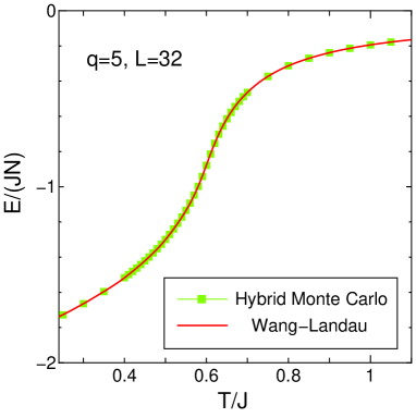
Figure 5: Comparison of temperature dependence of $E$ for $q=5$ with $L=32$ calculated by the hybrid Monte Carlo method and by the Wang-Landau method.

III.3 Correlation Ratio

Since the possibility of the extra first-order transition was ruled out, we next study the behavior of the KT transition. We here calculate the ratio of the correlation function Tomita02 defined as

$$R(L,T)=\frac{G(L/2,T)}{G(L/4,T)},$$ (4)

where $G(r,T)$ is the spin-spin correlation function in the $xy$ plane with the distance $r$,

$$G(r,T)=\langle S^{x}_{i}S^{x}_{i+r}+S^{y}_{i}S^{y}_{i+r}\rangle.$$ (5)

Here, $\langle\cdots\rangle$ denotes the thermal average. Starting from the scaling behavior of the correlation function of finite system with system size $L$,

$$G(r,T)\sim r^{-(D-2+\eta)}\ h(r/L,\xi/L),$$ (6)

we can obtain scaling properties of the correlation ratio $R(L,T)$, Eq. (4), Tomita02 . Here, $\xi$ is the correlation length, $\eta$ is the decay critical exponent and $D$ is the spatial dimension.

If we plot the temperature dependence of the correlation ratio for the systems showing the KT transition, for $T<T_{\rm KT}$ the correlation ratio has no size dependence, but for $T>T_{\rm KT}$ it depends on $L$. This comes from the fact that the correlation function decays as a power of the distance at all the temperatures below the KT transition point. The Binder ratio Binder has the same properties, but corrections are much smaller for the correlation ratio Tomita02 . Other possible choices are the helicity modulus and the ratio of the second moment correlation length to $L$, that is, $\xi_{L}/L$ Hasen05 . We plot the temperature dependence of the ratio of correlation function for $q=3$ in Fig. 6. The system sizes are $L$ = 16, 32, 64 and 128. We find a typical behavior of the KT transition; that is, for $T/J<0.6$ the correlation ratio has little size dependence, whereas for $T/J>0.6$ it depends on size, which suggests the critical temperature as $T_{\rm KT}/J\simeq 0.60$

Figure 6: Temperature dependence of the correlation ratio $R(L,T)$ of the 2D generalized XY model for $q$=3. The system sizes $L$ are 16, 32, 64 and 128.

III.4 FSS of Correlation Ratio

The finite-size scaling (FSS) is often used to analyze the KT transition. Assuming the KT form of the divergence of the correlation length as $\xi\propto\exp(c/\sqrt{|T-T_{\rm KT}|})$, we may plot the correlation ratio as a function of $L/\exp(c/\sqrt{|T-T_{\rm KT}|})$ for each size $L$. Then, if we choose $T_{\rm KT}$ (and $c$) such that all the data are collapsed on a single curve, we can determine $T_{\rm KT}$. Actually, we estimate $T_{\rm KT}$ as $T_{\rm KT}/J=0.60(1)$ for $q=3$, where the numbers in parentheses denote the errors in the last digit.

Here we do not go further into the usual FSS approach. Instead we employ the FSS without estimating $T_{\rm KT}$ to investigate the universality of the KT transition in detail. We focus on the FSS property of the ratio of the correlation ratio of different sizes, that is, $R(2L,T)/R(L,T)$. Such FSS was employed in the analysis of Potts model Caraccido ; Salas , but no attempt has been made for the KT transition. We note that in the KT transition, logarithmic corrections KT2 ; Janke might not be small. We plot $R(2L,T)/R(L,T)$ as a function of $R(L,T)$ in Fig. 7 for $q=1$ and $q=5$. The lattice size pairs $L$-$2L$ are indicated in the inset of the figure, such as 16-32. The value of $R(2L,T)/R(L,T)$ remains 1 for $R(L,T)\sim 1$, which corresponds to low temperature. The value of $R(2L,T)/R(L,T)$ deviates from 1 for smaller $R(L,T)$, which means $T>T_{\rm KT}$. All the data for $L$ = 16, 32 and 64 are collapsed on a single curve for both $q$=1 and $q$=5. That is, the FSS is very well.

Since the FSS plots of $q=1$ and $q=5$ look the same in Fig. 7, we try a universal FSS plot. We plot both data for $q=1$ and $q=5$ in the single figure, Fig. 8, where system sizes are $L$=16, 32 and 64. In Fig. 8, not only the data for $q=1$ (classical XY model) and $q=5$, but also those for $q=0$ (planar rotator model) and $q=10$ are plotted. All the data with different $q$ are collapsed on a single curve within error bars. It means that the universal FSS is satisfied for $q$=0, 1, 5 and 10. This is the first direct demonstration of the universality of the planar rotator model ($q=0$) and the classical XY model ($q=1$). Thus, we conclude that the generalized XY model clearly shows the universality of the KT transition at least for $q\leq 10$. From the universal FSS we can make the following statement. Although the KT transition points are different for each $q$, the value of the correlation ratio at the KT transition point is the same for all $q$.

Figure 7: FSS plot of $R(2L,T)/R(L,T)$ versus $R(L,T)$ of the 2D generalized XY model for $q$=1 and 5. The pair of system sizes $L$-$2L$ are 16-32, 32-64 and 64-128.

Figure 8: Universal FSS plot of $R(2L,T)/R(L,T)$ versus $R(L,T)$ of the 2D generalized XY model for $q$=0 (planar rotator model), 1 (XY model), 5 and 10. The pair of system sizes $L$-$2L$ are 16-32, 32-64 and 64-128.

III.5 Large $q$ behavior

We have confirmed the universal behavior of the KT transition at least for $q\leq 10$. But we saw in Fig. 3 that the transition becomes sharper for larger $q$. Now we study the generalized XY model for large enough $q$. We plot the energy DOS $\ln(g(E))$ for $q$ = 1, 10, 50 and 100 in Fig. 9, where the system size $L$ is fixed as 16. We find that $\ln(g(E))$ becomes a shape of triangle for larger $q$. The slope of the triangle becomes steeper with the increase of $q$. To check whether there exists a first-order transition or not for $q=100$, we follow the method shown in subsection III B. We give the energy dependence of $\ln(g(E))-\beta E$ for $L$ = 12, 16, 24, 32 and 48 in Fig. 10. In this plot, the data for different size are shifted vertically to make the structure clearly visible. We found a small double maximum structure in a short range of temperature. We note that the scale of vertical axis is much smaller than that of Fig. 4 or 9. The temperature was chosen such that the height of two maximum is the same, that is, $T/J$ is 0.3957, 0.3954, 0.3949 and 0.3948 for $L$ = 16, 24, 32 and 48, respectively. Although there exists double maximum in Fig. 10, the difference of maximum and minimum values of $\ln(g(E))-\beta E$ becomes smaller with increasing the lattice size. If a first-order transition occurs, the difference of maximum and minimum values of $\ln(g(E))-\beta E$ is expected to be proportional to $L^{D-1}$, where $D$ is the spatial dimension; $D$ is two in the present study. This means that the $q=100$ generalized XY model shows a behavior close to a first-order transition, but it is not a true first-order transition.

Figure 9: Energy DOS $g(E)$ for $q$ = 1, 10, 50 and 100. The system size $L$ is 16.

Figure 10: Plot of $\ln(g(E))-\beta E$ as a function of $E$ for $q$= 100 and $L$=12, 16, 24, 32 and 48. The temperature was chosen such that the height of two maximum is the same.

It is interesting to investigate the behavior of the KT transition for $q=100$. We plot the temperature dependence of the correlation ratio for $L$ = 16, 24, 32, 48 and 64 in Fig. 11. The hybrid Monte Carlo simulation is not effective because the transition is close to the first order in this case. Thus, we have used the Wang-Landau method to calculate the correlation ratio in Fig. 11, although the system size we can treat is limited. Since the size dependence is small for lower temperatures, we can say that Fig. 11 shows a behavior of KT transition, but we also observe a deviation from the KT behavior. It seems that the curves with different sizes do not merge but cross for low temperatures. The FSS plot of $R(2L,T)/R(L,T)$, which is shown in the inset of Fig. 11, deviates from the universal FSS plot given in Fig. 8. Since the deviations are larger for smaller $L$, they can be the corrections to FSS. It seems that the KT transition is recovered only in the thermodynamic limit for large enough $q$.

Figure 11: Temperature dependence of the correlation ratio $R(L,T)$ of the 2D generalized XY model for $q$=100. The system sizes $L$ are 16, 24, 32, 48 and 64. The FSS plot of $R(2L,T)/R(L,T)$ is shown in the inset.

IV Summary and Discussions

We have studied the 2D generalized XY model on the square lattice using the Monte Carlo methods. The behavior of the phase transitions with the change of the generalized parameter $q$ has been carefully checked by using both the hybrid canonical Monte Carlo method and the Wang-Landau method. The results of the temperature dependence of the energy and the specific heat show no sign of the first-order transition for all $q$; moreover, the careful check with the Wang-Landau method yields the same result. We have concluded that only the KT transition occurs in the 2D generalized XY model, which is contrary to the conclusion of Ref. gXY_MC but is consistent with original proposal by Romano and Zagrebnov Romano .

Since it has been made clear that there exists only a single KT transition, we have made the FSS analysis without assuming the transition temperature Caraccido ; Salas paying a special attention to the universality. We have studied the ratio of the correlation ratio of two sizes; namely, $R(2L,T)/R(L,T)$ versus $R(L,T)$. We have obtained that all the data for different $L$ are collapsed on a single curve for each $q$, which indicates that the FSS works well. Moreover, such curves with different $q$ are universal for all $q$ including the XY model ($q$=1) and the planar rotator model ($q$=0).

We have made a detailed analysis for the large $q$ behavior with the Wang-Landau method. When $q$ is large enough, the graph of the logarithm of energy DOS, $\ln(g(E))$, approaches the shape of triangle. Although there is a small double maximum in the plot of $\ln(g(E))-\beta E$, the free energy barrier becomes smaller for larger system size. It means that the transition is not a first order transition. From the analysis of the correlation ratio, the transition is like KT type, but the corrections to FSS are not negligible for larger $q$.

From the shape of Hamiltonian, Eq. (2), we see that for small $q$ the microscopic states apart from the $xy$ plane also contribute to the $xy$ coupling $\cos(\phi_{i}-\phi_{j})$ to some extent, whereas only the microscopic states near the $xy$ plane contribute to the $xy$ coupling for large $q$, due to the factor $(\sin\theta)^{q}$. This is the reason why $\ln(g(E))$ becomes a shape of triangle for larger $q$. In other words, for large $q$, the proportion of redundant states becomes larger as far as the $xy$ coupling is concerned. Recently, the role of invisible states, or the redundant states, was investigated for the Potts model Tamura . It was discussed that the order of transition changes from the second order to the first order when the number of invisible states increases. It will be an interesting problem to make clear the role of redundant states in the case of the KT transition.

References

- (1) Berezinskii V L 1971 Zh. Eksp. Teor. Fiz. 61 1144 [1972 JETP 34 610]
- (2) Kosterlitz J M and Thouless D J 1973 J. Phys. C: Solid State Phys. 6 1181
- (3) Kosterlitz J M 1974 J. Phys. C: Solid State Phys. 7 1046
- (4) Weber H and Minnhagen P 1988 Phys. Rev. B 37 5986
- (5) Olsson P 1995 Phys. Rev. B 52 4526
- (6) Hasenbusch M and Pinn K 1997 J. Phys. A: Math. Gen. 30 63
- (7) Hasenbusch M 2005 J. Phys. A: Math. Gen. 38 5869
- (8) Domany E, Schick M and Swendsen R H 1984 Phys. Rev. Lett. 52 1535
- (9) Sinha S and Roy S K 2010 Phys. Rev. E 81 022102
- (10) Sinha S and Roy S K 2010 Phys. Rev. E 81 041120
- (11) Romano S and Zagrebnov V 2002 Phys. Lett A 301 402
- (12) Mól L A S, Pereira A R and Moura-Melo W A 2003 Phys. Lett. A 319 114
- (13) Chamati H, Romano S, Mól L A S and Pereira A R 2005 Europhys. Lett. 72 62
- (14) Mól L A S, Pereira A R, Chamati H and Romano S 2006 Eur. Phys. J. B 50 541
- (15) Swendsen R H and Wang J S 1987 Phys. Rev. Lett. 58 86
- (16) Wolff U 1989 Phys. Rev. Lett. 62 361
- (17) Wang F and Landau D P 2001 Phys. Rev. Lett. 86 2050
- (18) Kasteleyn P W and Fortuin C M 1969 J. Phys. Soc. Jpn. Suppl. 26 11; Fortuin C M and Kasteleyn P W 1972 Physica 57 536
- (19) Tomita Y and Okabe Y 2002 Phys. Rev. B 66 180401(R)
- (20) Berg B A and Neuhaus T 1992 Phys. Rev. Lett. 68 9
- (21) Borgs C and Janke W 1992 J. Phys. (France) I 2 2011
- (22) Yamaguchi C and Okabe Y 2001 J. Phys. A: Math. Gen. 34 8781
- (23) Okabe Y and Otsuka H 2006 J. Phys. A: Math. Gen. 39 9093
- (24) Binder K 1981 Z. Phys. B 43 119
- (25) Caraccido S, Edwards R G, Ferreira S J, Pelissetto A and Sokal A D 1995 Phys. Rev. Lett. 74 2969
- (26) Salas J and Sokal A D 1997 J. Stat. Phys. 88 567
- (27) Janke W 1997 Phys. Rev. B 55 3580
- (28) Tamura R, Tanaka S and Kawashima N 2010 Prog. Theor. Phys. 124 381