SOLVING A GENERALIZED HERON PROBLEM
BY MEANS OF CONVEX ANALYSIS
BORIS S. MORDUKHOVICH, NGUYEN MAU NAM and JUAN SALINAS

Abstract The classical Heron problem states: on a given straight line in the plane, find a point $C$ such that the sum of the distances from $C$ to the given points $A$ and $B$ is minimal. This problem can be solved using standard geometry or differential calculus. In the light of modern convex analysis, we are able to investigate more general versions of this problem. In this paper we propose and solve the following problem: on a given nonempty closed convex subset of $I\!\!R^{s}$, find a point such that the sum of the distances from that point to $n$ given nonempty closed convex subsets of $I\!\!R^{s}$ is minimal.

1 Problem Formulation

Heron from Alexandria (10–75 AD) was “a Greek geometer and inventor whose writings preserved for posterity a knowledge of the mathematics and engineering of Babylonia, ancient Egypt, and the Greco-Roman world” (from the Encyclopedia Britannica). One of the geometric problems he proposed in his Catroptica was as follows: find a point on a straight line in the plane such that the sum of the distances from it to two given points is minimal.

Recall that a subset $\Omega$ of $I\!\!R^{s}$ is called convex if $\lambda x+(1-\lambda)y\in\Omega$ whenever $x$ and $y$ are in $\Omega$ and $0\leq\lambda\leq 1$. Our idea now is to consider a much broader situation, where two given points in the classical Heron problem are replaced by finitely many closed and convex subsets $\Omega_{i},\;i=1,\ldots,n$, and the given line is replaced by a given closed and convex subset $\Omega$ of $I\!\!R^{s}$. We are looking for a point on the set $\Omega$ such that the sum of the distances from that point to $\Omega_{i},\;i=1,\ldots,n,$ is minimal.

The distance from a point $x$ to a nonempty set $\Omega$ is understood in the conventional way

$$d(x;\Omega)=\inf\big{\{}||x-y||\;\big{|}\;y\in\Omega\big{\}},$$ (1.1)

where $||\cdot||$ is the Euclidean norm in $I\!\!R^{s}$. The new generalized Heron problem is formulated as follows:

$$\mbox{minimize }\;D(x):=\sum_{i=1}^{n}d(x;\Omega_{i})\;\mbox{ subject to }\;x\in\Omega,$$ (1.2)

where all the sets $\Omega$ and $\Omega_{i}$, $i=1,\ldots,n$, are nonempty, closed, and convex; these are our standing assumptions in this paper. Thus (1.2) is a constrained convex optimization problem, and hence it is natural to use techniques of convex analysis and optimization to solve it.

2 Elements of Convex Analysis

In this section we review some basic concepts of convex analysis used in what follows. This material and much more can be found, e.g., in the books [2, 3, 5].

Let $f\colon I\!\!R^{s}\to\overline{I\!\!R}:=(-\infty,\infty]$ be an extended-real-valued function, which may be infinite at some points, and let

$$\mbox{dom }f:=\big{\{}x\in I\!\!R^{s}\;\big{|}\;f(x)<\infty\big{\}}$$

be its effective domain. The epigraph of $f$ is a subset of $I\!\!R^{s}\times I\!\!R$ defined by

$$\mbox{epi }f:=\big{\{}(x,\alpha)\in I\!\!R^{s+1}\;\big{|}\;x\in\mbox{dom }f\;\mbox{ and }\;\alpha\geq f(x)\big{\}}.$$

The function $f$ is closed if its epigraph is closed, and it is convex is its epigraph is a convex subset of $I\!\!R^{s+1}$. It is easy to check that $f$ is convex if and only if

$$f\big{(}\lambda x+(1-\lambda)y\big{)}\leq\lambda f(x)+(1-\lambda)f(y)\;\mbox{ for all }\;x,y\in\mbox{dom }f\;\mbox{ and }\;\lambda\in[0,1].$$

Furthermore, a nonempty closed subset $\Omega$ of $I\!\!R^{s}$ is convex if and only if the corresponding distance function $f(x)=d(x;\Omega)$ is a convex function. Note that the distance function $f(x)=d(x;\Omega)$ is Lipschitz continuous on $I\!\!R^{s}$ with modulus one, i.e.,

$$|f(x)-f(y)|\leq||x-y||\;\mbox{ for all }\;x,y\in I\!\!R^{s}.$$

A typical example of an extended-real-valued function is the set indicator function

$$\delta(x;\Omega):=\begin{cases}0&\text{if }\;x\in\Omega,\\ \infty&\text{otherwise.}\end{cases}$$ (2.1)

It follows immediately from the definitions that the set $\Omega\subset I\!\!R^{s}$ is closed (resp. convex) if and only if the indicator function (2.1) is closed (resp. convex).

An element $v\in I\!\!R^{s}$ is called a subgradient of a convex function $f\colon I\!\!R^{s}\to\overline{I\!\!R}$ at $\bar{x}\in\mbox{dom}f$ if it satisfies the inequality

$$\langle v,x-\bar{x}\rangle\leq f(x)-f(\bar{x})\;\mbox{ for all }\;x\in I\!\!R^{s},$$ (2.2)

where $\langle\cdot,\cdot\rangle$ stands for the usual scalar product in $I\!\!R^{s}$. The set of all the subgradients $v$ in (2.2) is called the subdifferential of $f$ at $\bar{x}$ and is denoted by $\partial f(\bar{x})$. If $f$ is convex and differentiable at $\bar{x}$, then $\partial f(\bar{x})=\{\nabla f(\bar{x})\}$.

A well-recognized technique in optimization is to reduce a constrained optimization problem to an unconstrained one using the indicator function of the constraint. Indeed, $\bar{x}\in\Omega$ is a minimizer of the constrained optimization problem:

$$\mbox{minimize }\;f(x)\;\mbox{ subject to }\;x\in\Omega$$ (2.3)

if and only if it solves the unconstrained problem

$$\mbox{minimize }\;f(x)+\delta(x;\Omega),\;\;x\in I\!\!R^{s}.$$ (2.4)

By the definitions, for any convex function $\varphi\colon I\!\!R^{s}\to\overline{I\!\!R}$,

$$\bar{x}\;\mbox{ is a minimizer of }\;\varphi\;\mbox{ if and only if }\;0\in\partial\varphi(\bar{x}),$$ (2.5)

which is nonsmooth convex counterpart of the classical Fermat stationary rule. Applying (2.5) to the constrained optimization problem (2.3) via its unconstrained description (2.4) requires the usage of subdifferential calculus. The most fundamental calculus result of convex analysis is the following Moreau-Rockafellar theorem for representing the subdifferential of sums.

Theorem 2.1

Let $\varphi_{i}\colon I\!\!R^{s}\to\overline{I\!\!R}$, $i=1,\ldots,m$, be closed convex functions. Assume that there is a point $\bar{x}\in\cap_{i=1}^{n}\mbox{\rm dom}\,\varphi_{i}$ at which all but $($except possibly one$)$ of the functions $\varphi_{1},\ldots,\varphi_{m}$ are continuous. Then we have the equality

$$\partial\Big{(}\sum_{i=1}^{m}\varphi_{i}\Big{)}(\bar{x})=\sum_{i=1}^{m}\partial\varphi_{i}(\bar{x}).$$

Given a convex set $\Omega\subset I\!\!R^{s}$ and a point $\bar{x}\in\Omega$, the corresponding geometric counterpart of (2.2) is the normal cone to $\Omega$ at $\bar{x}$ defined by

$$N(\bar{x};\Omega):=\big{\{}v\in I\!\!R^{s}\big{|}\;\langle v,x-\bar{x}\rangle\leq 0\;\mbox{ for all }\;x\in\Omega\big{\}}.$$ (2.6)

It easily follows from the definitions that

$$\partial\delta(\bar{x};\Omega)=N(\bar{x};\Omega)\mbox{ for every }\bar{x}\in\Omega,$$ (2.7)

which allows us, in particular, to characterize minimizers of the constrained problem (2.3) in terms of the subdifferential (2.2) of $f$ and the normal cone (2.6) to $\Omega$ by applying Theorem 2.1 to the function $\varphi(x)=f(x)+\delta(x;\Omega)$ in (2.5).

Finally in this section, we present a useful formula for computing the subdifferential of the distance function (1.1) via the unique Euclidean projection

$$\Pi(\bar{x};\Omega):=\big{\{}x\in\Omega\;\big{|}\;||x-\bar{x}||=d(x;\Omega)\big{\}}$$ (2.8)

of $\bar{x}\in I\!\!R^{s}$ on the closed and convex set $\Omega\subset I\!\!R^{s}$.

Proposition 2.2

Let $\Omega\neq\emptyset$ be a closed and convex of $I\!\!R^{s}$. Then

$$\partial\mbox{d}(\bar{x};\Omega)=\left\{\begin{array}[]{lr}\Big{\{}\dfrac{\bar{x}-\Pi(\bar{x};\Omega)}{d(\bar{x};\Omega)}\Big{\}}&\mbox{ if }\;\bar{x}\notin\Omega,\\ \\ N(\bar{x};\Omega)\cap I\!\!B&\mbox{ if }\;\bar{x}\in\Omega,\end{array}\right.$$

where $I\!\!B$ is the closed unit ball of $I\!\!R^{s}$.

3 Optimal Solutions to the Generalized Heron Problem

In this section we derive efficient characterizations of optimal solutions to the generalized Heron problem (1.2), which allow us to completely solve this problem in some important particular settings.

First let us present general conditions that ensure the existence of optimal solutions to (1.2).

Proposition 3.1

Assume that one of the sets $\Omega$ and $\Omega_{i}$, $i=1,\ldots,n$, is bounded. Then the generalized Heron problem (1.2) admits an optimal solution.

Proof. Consider the optimal value

$$\gamma:=\inf_{x\in\Omega}D(x)$$

in (1.2) and take a minimizing sequence $\{x_{k}\}\subset\Omega$ with $D(x_{k})\to\gamma$ as $k\to\infty$. If the constraint set $\Omega$ is bounded, then by the classical Bolzano-Weierstrass theorem the sequence $\{x_{k}\}$ contains a subsequence converging to some point $\bar{x}$, which belongs to the set $\Omega$ due to it closedness. Since the function $D(x)$ in (1.2) is continuous, we have $D(\bar{x})=\gamma$, and thus $\bar{x}$ is an optimal solution to (1.2).

It remains to consider the case when one of sets $\Omega_{i}$, say $\Omega_{1}$, is bounded. In this case we have for the above sequence $\{x_{k}\}$ when $k$ is sufficiently large that

$$d(x_{k};\Omega_{1})\leq D(x_{k})<\gamma+1,$$

and thus there exists $w_{k}\in\Omega_{1}$ with $||x_{k}-w_{k}||<\gamma+1$ for such indexes $k$. Then

$$||x_{k}||<||w_{k}||+\gamma+1,$$

which shows that the sequence $\{x_{k}\}$ is bounded. The existence of optimal solutions follows in this case from the arguments above. $\hfill\triangle$

To characterize in what follows optimal solutions to the generalized Heron problem (1.2), for any nonzero vectors $u,v\in I\!\!R^{s}$ define the quantity

$$\cos(v,u):=\dfrac{\langle v,u\rangle}{||v||\cdot||u||}.$$ (3.1)

We say that $\Omega$ has a tangent space at $\bar{x}$ if there exists a subspace $L=L(\bar{x})\neq\{0\}$ such that

$$N(\bar{x};\Omega)=L^{\perp}:=\big{\{}v\in I\!\!R^{s}\big{|}\;\langle v,u\rangle=0\;\mbox{ whenever }\;u\in L\big{\}}.$$ (3.2)

The following theorem gives necessary and sufficient conditions for optimal solutions to (1.2) in terms of projections (2.8) on $\Omega_{i}$ incorporated into quantities (3.1). This theorem and its consequences are also important in verifying the validity of numerical results in the Section 3.

Theorem 3.2

Consider problem (1.2) in which

$$\Omega_{i}\cap\Omega=\emptyset\;\mbox{ for all }\;i=1,\ldots,n.$$ (3.3)

Given $\bar{x}\in\Omega$, define the vectors

$$a_{i}(\bar{x}):=\dfrac{\bar{x}-\Pi(\bar{x};\Omega_{i})}{d(\bar{x};\Omega_{i})}\neq 0,\quad i=1,\ldots,n,$$ (3.4)

Then $\bar{x}\in\Omega$ is an optimal solution to the generalized Heron problem (1.2) if and only if

$$-\sum_{i=1}^{n}a_{i}(\bar{x})\in N(\bar{x};\Omega).$$ (3.5)

Suppose in addition that the constraint set $\Omega$ has a tangent space $L$ at $\bar{x}$. Then (3.5) is equivalent to

$$\sum_{i=1}^{n}\cos\big{(}a_{i}(\bar{x}),u\big{)}=0\;\mbox{ whenever }\;u\in L\setminus\{0\}.$$ (3.6)

Proof. Fix an optimal solution $\bar{x}$ to problem (1.2) and equivalently describe it as an optimal solution to the following unconstrained optimization problem:

$$\mbox{minimize }\;D(x)+\delta(x;\Omega),\quad x\in I\!\!R^{s}.$$ (3.7)

Applying the generalized Fermat rule (2.5) to (3.7), we characterize $\bar{x}$ by

$$0\in\partial\Big{(}\sum_{i=1}^{n}d(\cdot;\Omega_{i})+\delta(\cdot;\Omega)\Big{)}(\bar{x}).$$ (3.8)

Since all of the functions $d(\cdot;\Omega_{i}),\;i=1,\ldots,n$, are convex and continuous, we employ the subdifferential sum rule of Theorem 2.1 to (3.8) and arrive at

$$\begin{array}[]{ll}0\in\partial\big{(}D+\delta(\cdot,\Omega)\big{)}(\bar{x})&=\displaystyle\sum_{i=1}^{n}\partial d(\bar{x};\Omega_{i})+N(\bar{x};\Omega)\\ &=\displaystyle\sum_{i=1}^{n}a_{i}(\bar{x})+N(\bar{x};\Omega),\end{array}$$ (3.11)

where the second representation in (3.11) is due to (2.7) and the subdifferential description of Proposition 2.2 with $a_{i}(\bar{x})$ defined in (3.4). It is obvious that (3.11) and (3.5) are equivalent.

Suppose in addition that the constraint set $\Omega$ has a tangent space $L$ at $\bar{x}$. Then the inclusion (3.5) is equivalent to

$$0\in\sum_{i=1}^{n}a_{i}(\bar{x})+L^{\perp},$$

which in turn can be written in the form

$$\Big{\langle}\sum_{i=1}^{n}a_{i}(\bar{x}),u\Big{\rangle}=0\;\mbox{ for all }\;u\in L.$$

Taking into account that $||a_{i}(\bar{x})||=1$ for all $i=1,\ldots,n$ by (3.4) and assumption (3.3), the latter equality is equivalent to

$$\sum_{i=1}^{n}\dfrac{\langle a_{i}(\bar{x}),v\rangle}{||a_{i}(\bar{x})||\cdot||u||}=0\;\mbox{ for all }\;u\in L\setminus\{0\},$$

which gives (3.6) due to the notation (3.1) and thus completes the proof of the theorem. $\hfill\triangle$

To further specify the characterization of Theorem 3.2, recall that a set $A$ of $I\!\!R^{s}$ is an affine subspace if there is a vector $a\in A$ and a (linear) subspace $L$ such that $A=a+L$. In this case we say that $A$ is parallel to $L$. Note that the subspace $L$ parallel to $A$ is uniquely defined by $L=A-A=\{x-y\;|\;x\in A,\;y\in A\}$ and that $A=b+L$ for any vector $b\in A$.

Corollary 3.3

Let $\Omega$ be an affine subspace parallel to a subspace $L$, and let assumption (3.3) of Theorem 3.2 be satisfied. Then $\bar{x}\in\Omega$ is a solution to the generalized Heron problem (1.2) if and only if condition (3.6) holds.

Proof. To apply Theorem 3.2, it remains to check that $L$ is a tangent space of $\Omega$ at $\bar{x}$ in the setting of this corollary. Indeed, we have $\Omega=\bar{x}+L$, since $\Omega$ is an affine subspace parallel to $L$. Fix any $v\in N(\bar{x};\Omega)$ and get by (2.6) that $\langle v,x-\bar{x}\rangle\leq 0$ whenever $x\in\Omega$ and hence $\langle v,u\rangle\leq 0$ for all $u\in L$. Since $L$ is a subspace, the latter implies that $\langle v,u\rangle=0$ for all $u\in L$, and thus $N(\bar{x};\Omega)\subset L^{\perp}$. The opposite inclusion is trivial, which gives (3.2) and completes the proof of the corollary. $\hfill\triangle$

The underlying characterization (3.6) can be easily checked when the subspace $L$ in Theorem 3.2 is given as a span of fixed generating vectors.

Corollary 3.4

Let $L={\rm{span}}\{u_{1},\ldots,u_{m}\}$ with $u_{j}\neq 0$, $i=1,\ldots,m$, in the setting of Theorem 3.2. Then $\bar{x}\in\Omega$ is an optimal solution to the generalized Heron problem (1.2) if and only if

$$\sum_{i=1}^{n}\cos\big{(}a_{i}(\bar{x}),u_{j}\big{)}=0\;\mbox{ for all }\;j=1,\ldots,m.$$ (3.12)

Proof. We show that (3.6) is equivalent to (3.12) in the setting under consideration. Since (3.6) obviously implies (3.12), it remains to justify the opposite implication. Denote

$$a:=\sum_{i=1}^{n}a_{i}(\bar{x})$$

and observe that (3.12) yields the condition

$$\langle a,u_{j}\rangle=0\;\mbox{ for all }\;j=1,\ldots m,$$ (3.13)

since $u_{j}\neq 0$ for all $j=1,\ldots,m$ and $||a_{i}||=1$ for all $i=1,\ldots,n$. Taking now any vector $u\in L\setminus\{0\}$, we represent it in the form

$$u=\sum_{j=1}^{m}\lambda_{j}u_{j}\;\mbox{ with some }\;\lambda_{j}\in I\!\!R^{n}$$

and get from (3.13) the equalities

$$\langle a,u\rangle=\sum_{j=1}^{n}\lambda_{j}\langle a,u_{j}\rangle=0.$$

This justifies (3.6) and completes the proof of the corollary. $\hfill\triangle$

Let us further examine in more detail the case of two sets $\Omega_{1}$ and $\Omega_{2}$ in (1.2) with the normal cone to the constraint set $\Omega$ being a straight line generated by a given vector. This is a direct extension of the classical Heron problem to the setting when two points are replaced by closed and convex sets, and the constraint line is replaced by a closed convex set $\Omega$ with the property above. The next theorem gives a complete and verifiable solution to the new problem.

Theorem 3.5

Let $\Omega_{1}$ and $\Omega_{2}$ be subsets of $I\!\!R^{s}$ as $s\geq 1$ with $\Omega\cap\Omega_{i}=\emptyset$ for $i=1,2$ in (1.2). Suppose also that there is a vector $a\neq 0$ such that $N(\bar{x};\Omega)={\rm{span}}\{a\}$. The following assertions hold, where $a_{i}:=a_{i}(\bar{x})$ are defined in (3.4):

(i) If $\bar{x}\in\Omega$ is an optimal solution to (1.2), then

$$\mbox{either }\;a_{1}+a_{2}=0\;\mbox{ or }\;\cos(a_{1},a)=\cos\big{(}a_{2},a).$$ (3.14)

(ii) Conversely, if $s=2$ and

$$\mbox{either }\;a_{1}+a_{2}=0\;\mbox{ or }\;\big{[}a_{1}\neq a_{2}\;\mbox{ and }\;\cos(a_{1},a)=\cos(a_{2},a)\big{]},$$ (3.15)

then $\bar{x}\in\Omega$ is an optimal solution to the generalized Heron problem (1.2).

Proof. It follows from the above (see the proof of Theorem 3.2) that $\bar{x}\in\Omega$ is an optimal solution to (1.2) if and only if $-a_{1}-a_{2}\in N(\bar{x};\Omega)$. By the assumed structure of the normal cone to $\Omega$ the latter is equivalent to the alternative:

$$\mbox{either }\;a_{1}+a_{2}=0\;\mbox{ or }\;a_{1}+a_{2}=\lambda a\;\mbox{ with some }\;\lambda\neq 0.$$ (3.16)

To justify (i), let us show that the second equality in (3.16) implies the corresponding one in (3.14). Indeed, we have $||a_{1}||=||a_{1}||=1$, and thus (3.16) implies that

$$\lambda^{2}||a||^{2}=||a_{1}+a_{2}||^{2}=||a_{1}||^{2}+||a_{2}||^{2}+2\langle a_{1},a_{2}\rangle=2+2\langle a_{1},a_{2}\rangle.$$

The latter yields in turn that

$$\langle a_{1},\lambda a\rangle =\langle\lambda a-a_{2},\lambda a\rangle$$

$$=\lambda^{2}||a||^{2}-\lambda\langle a_{2},a\rangle$$

$$=2+2\langle a_{1},a_{2}\rangle-\lambda\langle a_{2},a\rangle$$

$$=2\langle a_{2},a_{2}\rangle+2\langle a_{1},a_{2}\rangle-\lambda\langle a_{2},a\rangle$$

$$=2\langle a_{2}+a_{1},a_{2}\rangle-\lambda\langle a_{2},a\rangle$$

$$=2\langle\lambda a,a_{2}\rangle-\lambda\langle a_{2},a\rangle=\langle a_{2},\lambda a\rangle,$$

which ensures that $\langle a_{1},a\rangle=\langle a_{2},a\rangle$ as $\lambda\neq 0$. This gives us the equality $\cos(a_{1},a)=\cos(a_{2},a)$ due to $||a_{1}||=||a_{2}||=1$ and $a\neq 0$. Hence we arrive at (3.14).

To justify (ii), we need to prove that the relationships in (3.15) imply the fulfillment of

$$-a_{1}-a_{2}\in N(\bar{x};\Omega)=\mbox{span}\{a\}.$$ (3.17)

If $-a_{1}-a_{2}=0$, then (3.17) is obviously satisfied. Consider the alternative in(3.15) when $a_{1}\neq a_{2}$ and $\cos(a_{1},a)=\cos(a_{2},a)$. Since we are in $I\!\!R^{2}$, represent $a_{1}=(x_{1},y_{1})$, $a_{2}=(x_{2},y_{2})$, and $a=(x,y)$ with two real coordinates. Then by (3.1) the equality $\cos(a_{1},a)=\cos(a_{2},a)$ can be written as

$$x_{1}x+y_{1}y=x_{2}x+y_{2}y,\;\mbox{ i.e., }\;(x_{1}-x_{2})x=(y_{2}-y_{1})y.$$ (3.18)

Since $a\neq 0$, assume without loss of generality that $y\neq 0$. By

$$||a_{1}||^{2}=||a_{2}||^{2}\Longleftrightarrow x_{1}^{2}+y_{1}^{2}=x_{2}^{2}+y_{2}^{2}$$

we have the equality $(x_{1}-x_{2})(x_{1}+x_{2})=(y_{2}-y_{1})(y_{2}+y_{1})$, which implies by (3.18) that

$$y(x_{1}-x_{2})(x_{1}+x_{2})=x(x_{1}-x_{2})(y_{2}+y_{1}).$$ (3.19)

Note that $x_{1}\neq x_{2}$, since otherwise we have from (3.18) that $y_{1}=y_{2}$, which contradicts the condition $a_{1}\neq a_{2}$ in (3.15). Dividing both sides of (3.19) by $x_{1}-x_{2}$, we get

$$y(x_{1}+x_{2})=x(y_{2}+y_{1}),$$

which implies in turn that

$$y(a_{1}+a_{2})=y(x_{1}+x_{2},y_{1}+y_{2})=\big{(}x(y_{1}+y_{2}),y(y_{1}+y_{2})\big{)}=(y_{1}+y_{2})a.$$

In this way we arrive at the representation

$$a_{1}+a_{2}=\dfrac{y_{1}+y_{2}}{y}a$$

showing that inclusion (3.17) is satisfied. This ensures the optimality of $\bar{x}$ in (1.2) and thus completes the proof of the theorem. $\hfill\triangle$

Finally in this section, we present two examples illustrating the application of Theorem 3.2 and Corollary 3.4, respectively, to solving the corresponding the generalized and classical Heron problems.

Example 3.6

Consider problem (1.2) where $n=2$, the sets $\Omega_{1}$ and $\Omega_{2}$ are two point $A$ and $B$ in the plane, and the constraint $\Omega$ is a disk that does not contain $A$ and $B$. Condition (3.5) from Theorem 3.2 characterizes a solution $M\in\Omega$ to this generalized Heron problem as follows. In the first case the line segment $AB$ intersects the disk; then the intersection is a optimal solution. In this case the problem may actually have infinitely many solutions. Otherwise, there is a unique point $M$ on the circle such that a normal vector $\overrightarrow{n}$ to $\Omega$ at $M$ is the angle bisector of angle $AMB$, and that is the only optimal solution to the generalized Heron problem under consideration; see Figure 1.

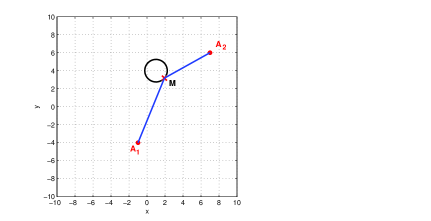
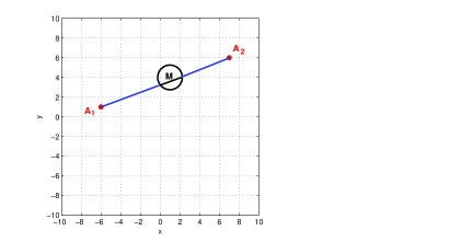
Figure 1: Generalized Heron Problem for Two Points with Disk Constraint.

Example 3.7

Consider problem (1.2), where $\Omega_{i}=\{A_{i}\}$, $i=1,\ldots,n$, are $n$ points in the plane, and where $\Omega={\cal L}\subset I\!\!R^{2}$ is a straight line that does not contain these points. Then, by Corollary 3.4 of Theorem 3.2, a point $M\in{\cal L}$ is a solution to this generalized Heron problem if and only if

$$\cos(\overrightarrow{MA_{1}},\overrightarrow{a})+\cdots+\cos(\overrightarrow{MA_{n}},\overrightarrow{a})=0,$$

where $\overrightarrow{a}$ is a direction vector of ${\cal L}$. Note that the latter equation completely characterizes the solution of the classical Heron problem in the plane in both cases when $A_{1}$ and $A_{2}$ are on the same side and different sides of ${\cal L}$; see Figure 2.

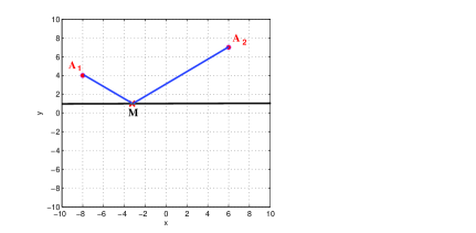
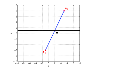
Figure 2: The Classical Heron Problem.

4 Numerical Algorithm and Its Implementation

In this section we present and justify an iterative algorithm to solve the generalized Heron problem (1.2) numerically and illustrate its implementations by using MATLAB in two important settings with disk and cube constraints. Here is the main algorithm.

Theorem 4.1

Let $\Omega$ and $\Omega_{i}$, $i=1,\ldots,n$, be nonempty closed convex subsets of $I\!\!R^{s}$ such that at least one of them is bounded. Picking a sequence $\{\alpha_{k}\}$ of positive numbers and a starting point $x_{1}\in\Omega$, consider the iterative algorithm:

$$x_{k+1}=\Pi\Big{(}x_{k}-\alpha_{k}\sum_{i=1}^{n}v_{ik};\Omega\Big{)},\quad k=1,2,\ldots,$$ (4.1)

where the vectors $v_{ik}$ in (4.1) are constructed by

$$v_{ik}:=\dfrac{x_{k}-\omega_{ik}}{d(x_{k};\Omega_{i})}\;\mbox{ with }\;\omega_{ik}:=\Pi(x_{k};\Omega_{i})\;\mbox{ if }\;x_{k}\notin\Omega_{i}$$ (4.2)

and $v_{ik}:=0$ otherwise. Assume that the given sequence $\{\alpha_{k}\}$ in (4.1) satisfies the conditions

$$\sum_{k=1}^{\infty}\alpha_{k}=\infty\;\mbox{ and }\;\sum_{k=1}^{\infty}\alpha_{k}^{2}<\infty.$$ (4.3)

Then the iterative sequence $\{x_{k}\}$ in (4.2) converges to an optimal solution of the generalized Heron problem (1.2) and the value sequence

$$V_{k}:=\min\big{\{}D(x_{j})\big{|}\;j=1,\ldots,k\big{\}}$$ (4.4)

converges to the optimal value $\widehat{V}$ in this problem.

Proof. Observe first of all that algorithm (4.1) is well posed, since the projection to a convex set used in (4.2) is uniquely defined. Furthermore, all the iterates $\{x_{k}\}$ in (4.1) are feasible; see the proof of Proposition 3.1. This algorithm and its convergence under conditions (4.3) are based on the subgradient method for convex functions in the so-called “square summable but not summable case” (see, e.g., [1]), the subdifferential sum rule of Theorem 2.1, and the subdifferential formula for the distance function given in Proposition 2.2. The reader can compare this algorithm and its justifications with the related developments in [4] for the numerical solution of the (unconstrained) generalized Fermat-Torricelli problem. $\hfill\triangle$

Let us illustrate the implementation of the above algorithm and the corresponding calculations to compute numerically optimal solutions in the following two characteristic examples.

Example 4.2

Consider the generalized Heron problem (1.2) for pairwise disjoint squares of right position in $I\!\!R^{2}$ (i.e., such that the sides of each square are parallel to the $x$-axis or the $y$-axis) subject to a given disk constraint. Let $c_{i}=(a_{i},b_{i})$ and $r_{i}$, $i=1,\ldots,n$, be the centers and the short radii of the squares under consideration. The vertices of the $i$th square are denoted by $q_{1i}=(a_{i}+r_{i},b_{i}+r_{i}),\;q_{2i}=(a_{i}-r_{i},b_{i}+r_{i}),\;q_{3i}=(a_{i}-r_{i},b_{i}-r_{i}),\;q_{4i}=(a_{i}+r_{i},b_{i}-r_{i})$. Let $r$ and $p=(\nu,\eta)$, be the radius and the center of the constraint. Then the subgradient algorithm (4.1) is written in this case as

$$x_{k+1}=\Pi\Big{(}x_{k}-\alpha_{k}\sum_{i=1}^{n}v_{ik};\Omega\Big{)},$$

where the projection $P(x,y):=\Pi((x,y);\Omega)$ is calculated by

$$P(x,y)=(w_{x}+\nu,w_{y}+\eta)\;\mbox{ with }\;w_{x}=\displaystyle\frac{r(x-\nu)}{\sqrt{(x-\nu)^{2}+(y-\eta)^{2}}}\;\mbox{ and }\;w_{y}=\displaystyle\frac{r(y-\eta)}{\sqrt{(x-\nu)^{2}+(y-\eta)^{2}}}.$$

The quantities $v_{ik}$ in the above algorithm are computed by

$$v_{ik}=\left\{\begin{array}[]{ll}0&\mbox{if }\;|x_{1k}-a_{i}|\leq r_{i}\;\mbox{ and }\;|x_{2k}-b_{i}|\leq r_{i},\\ \\ \displaystyle\frac{x_{k}-q_{1i}}{\|x_{k}-q_{1i}\|}&\mbox{if }\;x_{1k}-a_{i}>r_{i}\mbox{ and }\;x_{2k}-b_{i}>r_{i},\\ \\ \displaystyle\frac{x_{k}-q_{2i}}{\|x_{k}-q_{2i}\|}&\mbox{if }\;x_{1k}-a_{i}<-r_{i}\;\mbox{ and }\;x_{2k}-b_{i}>r_{i},\\ \\ \displaystyle\frac{x_{k}-q_{3i}}{\|x_{k}-q_{3i}\|}&\mbox{if }\;x_{1k}-a_{i}<-r_{i}\;\mbox{ and }\;x_{2k}-b_{i}<-r_{i},\\ \\ \displaystyle\frac{x_{k}-q_{4i}}{\|x_{k}-q_{4i}\|}&\mbox{if }\;x_{1k}-a_{i}>r_{i}\;\mbox{ and }\;x_{2k}-b_{i}<-r_{i},\\ \\ (0,1)&\mbox{if }\;|x_{1k}-a_{i}|\leq r_{i}\;\mbox{ and }\;x_{2k}-b_{i}>r_{i},\\ \\ (0,-1)&\mbox{if }\;|x_{1k}-a_{i}|\leq r_{i}\;\mbox{ and }\;x_{2k}-b_{i}<-r_{i},\\ \\ (1,0)&\mbox{if }\;|x_{1k}-a_{i}|>r_{i}\;\mbox{ and }\;|x_{2k}-b_{i}|\leq r_{i},\\ \\ (-1,0)&\mbox{if }\;|x_{1k}-a_{i}|<-r_{i}\;\mbox{ and }\;|x_{2k}-b_{i}|\leq r_{i}\\ \\ \end{array}\right.$$

for all $i=1,\ldots,n$ and $k=1,2,\ldots$ with the corresponding quantities $V_{k}$ defined by (4.4).

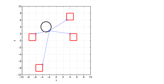
MATLAB RESULT
$k$	$x_{k}$	$V_{k}$
1	(-3,5.5)	30.99674
10	(-1.95277,2.92608)	26.14035
100	(-2.02866,2.85698)	26.13429
1000	(-2.03861,2.84860)	26.13419
10,000	(-2.03992,2.84750)	26.13419
100,000	(-2.04010,2.84736)	26.13419
200,000	(-2.04011,2.84735)	26.13419
400,000	(-2.04012,2.84734)	26.13419
600,000	(-2.04012,2.84734)	26.13419

Figure 3: Generalized Heron Problem for Squares with Disk Constraint.

For the implementation of this algorithm we develop a MATLAB program. The following calculations are done and presented below (see Figure 3 and the corresponding table) for the disk constraint $\Omega$ with center $(-3,4)$ and radius $1.5$, for the squares $\Omega_{i}$ with the same short radius $r=1$ and centers $(-7,1)$, $(-5,-8)$, (4,7), and (5,1), for the starting point $x_{1}=(-3,5.5)\in\Omega$, and for the sequence of $\alpha_{k}=1/k$ in (4.1) satisfying conditions (4.3). The optimal solution and optimal value computed up to five significant digits are $\bar{x}=(-2.04012,2.84734)$ and $\widehat{V}=26.13419$.

The next example concerns the generalized Heron problem for cubes with ball constraints in $I\!\!R^{3}$.

Example 4.3

Consider the generalized Heron problem (1.2) for pairwise disjoint cubes of right position in $I\!\!R^{3}$ subject to a ball constraint. In this case the subgradient algorithm (4.1) is

$$x_{k+1}=\Pi\Big{(}x_{k}-\alpha_{k}\sum_{i=1}^{n}v_{ik};\Omega\Big{)},$$

where the projection $\Pi((x,y,z);\Omega)$ and quantities $v_{ik}$ are computed similarly to Example 4.2.

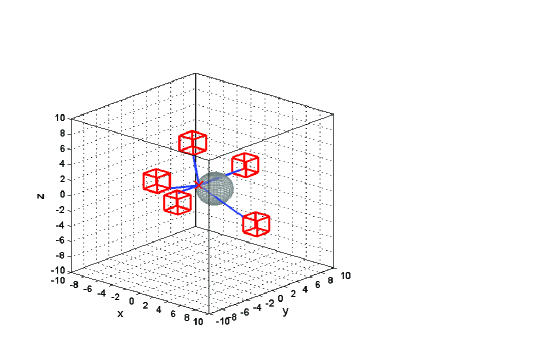
MATLAB RESULT
$k$	$x_{k}$	$V_{k}$
1	(2,2,0)	27.35281
1,000	(-0.68209,0.25502,0.69986)	24.74138
1,000,000	(-0.77641,0.31416,0.74508)	24.73757
2,000,000	(-0.77729,0.31480,0.74561)	24.73757
3,000,000	(-0.77769,0.31509,0.74584)	24.73757
3,500,000	(-0.77782,0.31518,0.74592)	24.73757
4,000,000	(-0.77792,0.31526,0.74598)	24.73757
4,500,000	(-0.77801,0.31532,0.74604)	24.73757
5,000,000	(-0.77808,0.31538,0.74608)	24.73757

Figure 4: Generalized Heron Problem for Cubes with Ball Constraint.

For the implementation of this algorithm we develop a MATLAB program. The Figure 4 and the corresponding figure present the calculation results for the ball constraint $\Omega$ with center $(0,2,0)$ and radius $2$, the cubes $\Omega_{i}$ with centers $(0,-4,0)$, $(6,2,-3)$, $(-3,-4,2)$, $(-5,4,4)$, and $(-1,8,1)$ with the same short radius $r=1$, the starting point $x_{1}=(2,2,0)$, and the sequence of $\alpha_{k}=1/k$ in (4.1) satisfying (4.3). The optimal solution and optimal value computed up to five significant digits are $\bar{x}=(-0.77808,0.31538,0.74608)$ and $\widehat{V}=24.73756$.

References

- [1] Bertsekas, D., Nedic, A., Ozdaglar, A.: Convex Analysis and Optimization. Athena Scientific, Boston, MA (2003)
- [2] Borwein, J.M., Lewis, A.S.: Convex Analysis and Nonlinear Optimization: Theory and Examples, 2nd edition. Springer, New York (2006)
- [3] Hiriart-Urruty, J.-B., Lemaréchal, C.: Fundamentals of Convex Analysis. Springer, Berlin (2001)
- [4] Mordukhovich, B.S., Nam, N.M.: Applications of variational analysis to a generalized Fermat-Torricelli problem. J. Optim. Theory Appl. 148, No. 3 (2011)
- [5] Rockafellar, R.T.: Convex Analysis. Princeton University Press, Princeton, NJ (1970)