Regularization Strategies and Empirical Bayesian Learning for MKL

\nameRyota Tomioka \emailtomioka@mist.i.u-tokyo.ac.jp
\nameTaiji Suzuki \emails-taiji@stat.t.u-tokyo.ac.jp
\addrDepartment of Mathematical Informatics, The University of Tokyo,
7-3-1, Hongo, Bunkyo-ku, Tokyo, 113-8656, Japan
Abstract

Multiple kernel learning (MKL), structured sparsity, and multi-task learning have recently received considerable attention. In this paper, we show how different MKL algorithms can be understood as applications of either regularization on the kernel weights or block-norm-based regularization, which is more common in structured sparsity and multi-task learning. We show that these two regularization strategies can be systematically mapped to each other through a concave conjugate operation. When the kernel-weight-based regularizer is separable into components, we can naturally consider a generative probabilistic model behind MKL. Based on this model, we propose learning algorithms for the kernel weights through the maximization of marginal likelihood. We show through numerical experiments that 2subscript2\ell_{2}-norm MKL and Elastic-net MKL achieve comparable accuracy to uniform kernel combination. Although uniform kernel combination might be preferable from its simplicity, 2subscript2\ell_{2}-norm MKL and Elastic-net MKL can learn the usefulness of the information sources represented as kernels. In particular, Elastic-net MKL achieves sparsity in the kernel weights.

1 Introduction

In many learning problems, the choice of feature representation, descriptors, or kernels plays a crucial role. The optimal representation is problem specific. For example, we can represent a web page as a bag-of-words, which might help us in classifying whether the page is discussing politics or economy; we can also represent the same page by the links provided in the page, which could be more useful in classifying whether the page is supporting political party A or B. Similarly in a visual categorization task, a color-based descriptor might be useful in classifying an apple from a lemon but not in discriminating an airplane from a car. Given that there is no single feature representation that works in every learning problem, it is crucial to combine them in a problem dependent manner for a successful data analysis.

In this paper, we consider the problem of combining multiple data sources in a kernel-based learning framework. More specifically, we assume that a data point x𝒳𝑥𝒳x\in{\mathcal{X}} lies in a space 𝒳𝒳\mathcal{X} and we are given M𝑀M candidate kernel functions km:𝒳×𝒳:subscript𝑘𝑚𝒳𝒳k_{m}:{\mathcal{X}}\times{\mathcal{X}}\rightarrow{\mathbb{R}} (m=1,,M𝑚1𝑀m=1,\ldots,M). Each kernel function corresponds to one data source. A conical combination of kmsubscript𝑘𝑚k_{m} (m=1,,M𝑚1𝑀m=1,\ldots,M) gives the combined kernel function k¯=m=1Mdmkm¯𝑘superscriptsubscript𝑚1𝑀subscript𝑑𝑚subscript𝑘𝑚\bar{k}=\sum_{m=1}^{M}d_{m}k_{m}, where dmsubscript𝑑𝑚d_{m} is a nonnegative weight. Our goal is to find a good set of kernel weights based on some training examples.

Various approaches have been proposed for the above problem under the name multiple kernel learning (MKL) (Lanckriet et al., 2004; Bach et al., 2004; Zien and Ong, 2007; Varma and Ray, 2007; Aflalo et al., 2009; Gehler and Nowozin, 2009; Kloft et al., 2009; Longworth and Gales, 2009; Cortes et al., 2009). Recently, Kloft et al. (2009, 2010) have shown that many MKL approaches can be understood as application of the penalty-based regularization (Tikhonov regularization) or constraint-based regularization (Ivanov regularization) on the kernel weights dmsubscript𝑑𝑚d_{m}. Meanwhile, there is a growing interest in learning under structured sparsity assumption (Yuan and Lin, 2006; Argyriou et al., 2008; Huang et al., 2009; Jacob et al., 2009; Jenatton et al., 2009), which employs another regularization based on the so-called block-norm.

Therefore, a natural question to ask is how these two regularization strategies are related to each other. For simple cases the correspondence is well known (see Bach et al. (2004, 2005); Kloft et al. (2009)). Moreover, in the context of structured sparsity, Micchelli et al. (2010) have proposed a more sophisticated class of penalty functions that employ both Tikhonov and Ivanov regularizations on the kernel weights and have shown the corresponding block-norm regularization. The first contribution of this paper is to show that under some mild assumptions the kernel-weight-based regularization and the block-norm-based regularization can be mapped to each other in a systematic manner through a concave conjugate operation.

All the regularization strategies we discussed so far is formulated as convex optimization problems. The second contribution of this paper is to propose a nonconvex regularizer based on the marginal likelihood. Although the overall minimization problem is nonconvex, we propose a iterative algorithm that alternately minimize two convex objectives. Although Bayesian approaches have been applied to MKL earlier in a transductive nonparametric setting by Zhang et al. (2004), and a setting similar to the relevance vector machine (Tipping, 2001) by Girolami and Rogers (2005); Damoulas and Girolami (2008), our formulation is more coherent with the correspondence between Gaussian process classification/regression and kernel methods (Rasmussen and Williams, 2006). Note that very recently Archambeau and Bach (2010); Urtasun (2010) also studied similar models.

This paper is structured as follows. In Section 2, we start from analyzing learning with fixed kernel combination. Then we discuss the two regularization strategies (kernel-weight-based regularization and block-norm-based regularization). Finally, we present our main result on the correspondence between the two formulations. In Section 3, we start from viewing the separable kernel-weight-based model as a hierarchical maximum a posteriori(MAP) estimation problem, and propose an empirical Bayesian approach for the same model. Furthermore, we show a connection to the general framework we discuss in Section 2. We numerically compare the proposed empirical Bayesian MKL and various MKL models on visual categorization tasks from the Caltech 101 dataset (Fei-Fei et al., 2004) using 1,760 kernel functions. Finally, we summarize our contributions in Section 5.

2 Multiple kernel learning frameworks and their connections

In this section, we first consider the problem of learning a classifier with a fixed kernel combination. Then we extend this framework to jointly optimize the kernel weights together with the classifier. Second, we consider the block-norm based regularization, which have been discussed in structured sparsity literature (including group lasso) (Yuan and Lin, 2006; Argyriou et al., 2008; Huang et al., 2009; Jacob et al., 2009; Jenatton et al., 2009). Our main concern is in how these two formulations are related to each other. We show two theorems (Theorem 1 and 7) that map the two formulations. Using these theorems, we show that previously proposed regularized MKL models can be systematically transformed from one formulation to another.

2.1 Learning with fixed kernel combination

We assume that we are given N𝑁N training examples (xi,yi)i=1Nsuperscriptsubscriptsubscript𝑥𝑖subscript𝑦𝑖𝑖1𝑁(x_{i},y_{i})_{i=1}^{N} where xisubscript𝑥𝑖x_{i} belongs to an input space 𝒳𝒳{\mathcal{X}} and yisubscript𝑦𝑖y_{i} belongs to an output space 𝒴𝒴{\mathcal{Y}} (usual settings are 𝒴={±1}𝒴plus-or-minus1{\mathcal{Y}}=\{\pm 1\} for classification and 𝒴=𝒴{\mathcal{Y}}={\mathbb{R}} for regression).

We first consider a learning problem with fixed kernel weights. More specifically, we fix non-negative kernel weights d1,d2,,dMsubscript𝑑1subscript𝑑2subscript𝑑𝑀d_{1},d_{2},\ldots,d_{M} and consider the RKHS ¯¯\bar{{\mathcal{H}}} corresponding to the combined kernel function k¯=m=1Mdmkm¯𝑘superscriptsubscript𝑚1𝑀subscript𝑑𝑚subscript𝑘𝑚\bar{k}=\sum_{m=1}^{M}d_{m}k_{m}. The squared RKHS norm of a function f¯¯𝑓\bar{f} in the combined RKHS ¯¯\bar{{\mathcal{H}}} can be represented as follows:

f¯¯2:=minf11,,fMMm=1Mfmm2dms.t.f¯=m=1Mfm,formulae-sequenceassignsuperscriptsubscriptnorm¯𝑓¯2subscriptsubscript𝑓1subscript1subscript𝑓𝑀subscript𝑀superscriptsubscript𝑚1𝑀superscriptsubscriptnormsubscript𝑓𝑚subscript𝑚2subscript𝑑𝑚st¯𝑓superscriptsubscript𝑚1𝑀subscript𝑓𝑚\displaystyle\|\bar{f}\|_{\bar{{\mathcal{H}}}}^{2}:=\min_{\begin{subarray}{c}f_{1}\in{\mathcal{H}}_{1},\\ \ldots,f_{M}\in{\mathcal{H}}_{M}\end{subarray}}\sum_{m=1}^{M}\frac{\|f_{m}\|_{{\mathcal{H}}_{m}}^{2}}{d_{m}}\quad{\rm s.t.}\,\,\bar{f}=\sum_{m=1}^{M}f_{m}, (1)

where msubscript𝑚{\mathcal{H}}_{m} is the RKHS that corresponds to the kernel function kmsubscript𝑘𝑚k_{m}. If dm=0subscript𝑑𝑚0d_{m}=0, the ratio fmm2/dmsuperscriptsubscriptnormsubscript𝑓𝑚subscript𝑚2subscript𝑑𝑚\|f_{m}\|_{{\mathcal{H}}_{m}}^{2}/d_{m} is defined to be zero if fmm=0subscriptnormsubscript𝑓𝑚subscript𝑚0\|f_{m}\|_{{\mathcal{H}}_{m}}=0 and infinity otherwise. See Sec 6 in Aronszajn (1950), and also Lemma 25 in Micchelli and Pontil (2005) for the proof. We also provide some intuition for a finite dimensional case in Appendix A.

Using the above representation, a supervised learning problem with a fixed kernel combination can be written as follows:

minimizef11,,fMM,bsubscriptminimizesubscript𝑓1subscript1subscript𝑓𝑀subscript𝑀𝑏\displaystyle\mathop{\mathrm{minimize}}_{\begin{subarray}{c}f_{1}\in{\mathcal{H}}_{1},\\ \ldots,f_{M}\in{\mathcal{H}}_{M},\\ b\in{\mathbb{R}}\end{subarray}} i=1N(yi,m=1Mfm(xi)+b)+C2m=1Mfmm2dm,superscriptsubscript𝑖1𝑁subscript𝑦𝑖superscriptsubscript𝑚1𝑀subscript𝑓𝑚subscript𝑥𝑖𝑏𝐶2superscriptsubscript𝑚1𝑀superscriptsubscriptnormsubscript𝑓𝑚subscript𝑚2subscript𝑑𝑚\displaystyle\sum_{i=1}^{N}\ell\left(y_{i},\textstyle\sum_{m=1}^{M}f_{m}(x_{i})+b\right)+\frac{C}{2}\sum_{m=1}^{M}\frac{\|f_{m}\|_{{\mathcal{H}}_{m}}^{2}}{d_{m}}, (2)

where :×:\ell:{\mathbb{R}}\times{\mathbb{R}}\rightarrow{\mathbb{R}} is a loss function and we assume that \ell is convex in the second argument; for example, the loss function can be the hinge loss H(yi,zi)=max(0,1yizi)subscript𝐻subscript𝑦𝑖subscript𝑧𝑖01subscript𝑦𝑖subscript𝑧𝑖\ell_{H}(y_{i},z_{i})=\max(0,1-y_{i}z_{i}), or the quadratic loss Q(yi,zi)=(yizi)2/(2σy2)subscript𝑄subscript𝑦𝑖subscript𝑧𝑖superscriptsubscript𝑦𝑖subscript𝑧𝑖22superscriptsubscript𝜎𝑦2\ell_{Q}(y_{i},z_{i})=(y_{i}-z_{i})^{2}/(2\sigma_{y}^{2}).

It might seem that we are making the problem unnecessarily complex by introducing M𝑀M functions fmsubscript𝑓𝑚f_{m} to optimize instead of simply optimizing over f¯¯𝑓\bar{f}. However, explicitly handling the kernel weights enables us to consider various regularization strategies on the weights as we see in the next subsection.

2.2 Kernel-weight-based regularization

Now we are ready to also optimize the kernel weights dmsubscript𝑑𝑚d_{m} in the above formulation. Clearly there is a need for regularization, because the objective (2) is a monotone decreasing function of the kernel weights dmsubscript𝑑𝑚d_{m}. Intuitively speaking, dmsubscript𝑑𝑚d_{m} corresponds to the complexity allowed for the m𝑚mth regression function fmsubscript𝑓𝑚f_{m}; the more complexity we allow, the better the fit to the training examples becomes. Thus without any constraint on dmsubscript𝑑𝑚d_{m}, we can get a severe overfitting problem.

Let h:+M{+}:subscriptsuperscript𝑀h:{\mathbb{R}}^{M}_{+}\rightarrow{\mathbb{R}}\cup\{+\infty\} be a function from a non-negative real vector 𝒅+M𝒅superscriptsubscript𝑀\boldsymbol{d}\in{\mathbb{R}}_{+}^{M} to a real number. One way to penalize the complexity is to minimize the objective (2) together with the regularizer h(𝒅)𝒅h(\boldsymbol{d}) as follows:

minimizef11,,fMM,b,𝒅+Msubscriptminimizeformulae-sequencesubscript𝑓1subscript1subscript𝑓𝑀subscript𝑀𝑏𝒅superscriptsubscript𝑀\displaystyle\mathop{\mathrm{minimize}}_{\begin{subarray}{c}f_{1}\in{\mathcal{H}}_{1},\ldots,f_{M}\in{\mathcal{H}}_{M},\\ b\in{\mathbb{R}},\\ \boldsymbol{d}\in{\mathbb{R}}_{+}^{M}\end{subarray}} i=1N(yi,m=1Mfm(xi)+b)+C2(m=1Mfmm2dm+h(𝒅)).superscriptsubscript𝑖1𝑁subscript𝑦𝑖superscriptsubscript𝑚1𝑀subscript𝑓𝑚subscript𝑥𝑖𝑏𝐶2superscriptsubscript𝑚1𝑀superscriptsubscriptnormsubscript𝑓𝑚subscript𝑚2subscript𝑑𝑚𝒅\displaystyle\sum_{i=1}^{N}\ell\left(y_{i},\textstyle\sum_{m=1}^{M}f_{m}(x_{i})+b\right)+\frac{C}{2}\left(\sum_{m=1}^{M}\frac{\|f_{m}\|_{{\mathcal{H}}_{m}}^{2}}{d_{m}}+h(\boldsymbol{d})\right). (3)

Note that if hh is a convex function, the above optimization problem is jointly convex in fmsubscript𝑓𝑚f_{m} and dmsubscript𝑑𝑚d_{m} (see Boyd and Vandenberghe (2004, Example 3.18))

Example 1 (psubscript𝑝\ell_{p}-norm MKL via Tikhonov regularization)

Let h(𝐝)=m=1Mdmp/p𝐝superscriptsubscript𝑚1𝑀superscriptsubscript𝑑𝑚𝑝𝑝h(\boldsymbol{d})=\sum_{m=1}^{M}d_{m}^{p}/p. Then we have

minimizef11,,fMM,b,𝒅+Msubscriptminimizeformulae-sequencesubscript𝑓1subscript1subscript𝑓𝑀subscript𝑀𝑏𝒅superscriptsubscript𝑀\displaystyle\mathop{\mathrm{minimize}}_{\begin{subarray}{c}f_{1}\in{\mathcal{H}}_{1},\ldots,f_{M}\in{\mathcal{H}}_{M},\\ b\in{\mathbb{R}},\\ \boldsymbol{d}\in{\mathbb{R}}_{+}^{M}\end{subarray}} i=1N(yi,m=1Mfm(xi)+b)+C2m=1M(fmm2dm+dmpp)superscriptsubscript𝑖1𝑁subscript𝑦𝑖superscriptsubscript𝑚1𝑀subscript𝑓𝑚subscript𝑥𝑖𝑏𝐶2superscriptsubscript𝑚1𝑀superscriptsubscriptnormsubscript𝑓𝑚subscript𝑚2subscript𝑑𝑚superscriptsubscript𝑑𝑚𝑝𝑝\displaystyle\sum_{i=1}^{N}\ell\left(y_{i},\textstyle\sum_{m=1}^{M}f_{m}(x_{i})+b\right)+\frac{C}{2}\sum_{m=1}^{M}\left(\frac{\|f_{m}\|_{{\mathcal{H}}_{m}}^{2}}{d_{m}}+\frac{d_{m}^{p}}{p}\right)

The special case p=1𝑝1p=1 was considered earlier in Varma and Ray (2007).

Example 2 (psubscript𝑝\ell_{p}-norm MKL via Ivanov regularization)

Let h(𝐝)=0𝐝0h(\boldsymbol{d})=0 if m=1Mdmp1superscriptsubscript𝑚1𝑀superscriptsubscript𝑑𝑚𝑝1\sum_{m=1}^{M}d_{m}^{p}\leq 1 and h(𝐝)=+𝐝h(\boldsymbol{d})=+\infty otherwise. Then we have

minimizef11,,fMM,b,𝒅+Msubscriptminimizeformulae-sequencesubscript𝑓1subscript1subscript𝑓𝑀subscript𝑀𝑏𝒅superscriptsubscript𝑀\displaystyle\mathop{\mathrm{minimize}}_{\begin{subarray}{c}f_{1}\in{\mathcal{H}}_{1},\ldots,f_{M}\in{\mathcal{H}}_{M},\\ b\in{\mathbb{R}},\\ \boldsymbol{d}\in{\mathbb{R}}_{+}^{M}\end{subarray}} i=1N(yi,m=1Mfm(xi)+b)+C2m=1Mfmm2dms.t.m=1Mdmp1.\displaystyle\sum_{i=1}^{N}\ell\left(y_{i},\textstyle\sum_{m=1}^{M}f_{m}(x_{i})+b\right)+\frac{C}{2}\sum_{m=1}^{M}\frac{\|f_{m}\|_{{\mathcal{H}}_{m}}^{2}}{d_{m}}\quad{\rm s.t.}\quad\sum_{m=1}^{M}d_{m}^{p}\leq 1.

This formulation was considered by Kloft et al. (2008, 2009). The special case p=2𝑝2p=2 was considered by Cortes et al. (2009).

Example 3 (Multi-task learning)

In this example, the linear combination inside the loss term is defined in a sample-dependent manner. More precisely, we assume that there are n𝑛n tasks, and each sample is associated with the l(i)𝑙𝑖l(i)th task. Let {\mathcal{H}} be an RKHS over the input space 𝒳𝒳{\mathcal{X}}. We consider M=n+1𝑀𝑛1M=n+1 functions f1,,fMsubscript𝑓1subscript𝑓𝑀f_{1},\ldots,f_{M}\in{\mathcal{H}} to model the task dependent component and the task independent component. The first n𝑛n functions f1,,fnsubscript𝑓1subscript𝑓𝑛f_{1},\ldots,f_{n}\in{\mathcal{H}} represent the task dependent components of the classifiers, and the last function fMsubscript𝑓𝑀f_{M}\in{\mathcal{H}} represents the component that is common to all tasks. Accordingly, the optimization problem can be expressed as follows:

minimizef11,,fMM,b,𝒅+Msubscriptminimizeformulae-sequencesubscript𝑓1subscript1subscript𝑓𝑀subscript𝑀𝑏𝒅superscriptsubscript𝑀\displaystyle\mathop{\mathrm{minimize}}_{\begin{subarray}{c}f_{1}\in{\mathcal{H}}_{1},\ldots,f_{M}\in{\mathcal{H}}_{M},\\ b\in{\mathbb{R}},\\ \boldsymbol{d}\in{\mathbb{R}}_{+}^{M}\end{subarray}} i=1N(yi,fl(i)(xi)+fM(xi)+b)+C2m=1Mfmm2dms.t.m=1Mdm1.\displaystyle\sum_{i=1}^{N}\ell\left(y_{i},f_{l(i)}(x_{i})+f_{M}(x_{i})+b\right)+\frac{C}{2}\sum_{m=1}^{M}\frac{\|f_{m}\|_{{\mathcal{H}}_{m}}^{2}}{d_{m}}\quad{\rm s.t.}\quad\sum_{m=1}^{M}d_{m}\leq 1.

Evgeniou and Pontil (2004); Evgeniou et al. (2005) proposed a related model that only has one parameter; they used dm=nλsubscript𝑑𝑚𝑛𝜆d_{m}=n\lambda for m=1,,n𝑚1𝑛m=1,\ldots,n and m=1ndm/n2+dM1superscriptsubscript𝑚1𝑛subscript𝑑𝑚superscript𝑛2subscript𝑑𝑀1\sum_{m=1}^{n}d_{m}/n^{2}+d_{M}\leq 1 instead of the constraint in the above formulation. However they did not discuss joint optimization of the hyperparameter λ𝜆\lambda and the classifier.

Example 4 (Wedge penalty)

Let h(𝐝)=m=1Mdm𝐝superscriptsubscript𝑚1𝑀subscript𝑑𝑚h(\boldsymbol{d})=\sum_{m=1}^{M}d_{m} if dmdm+1subscript𝑑𝑚subscript𝑑𝑚1d_{m}\geq d_{m+1} for all m=1,,M1𝑚1𝑀1m=1,\ldots,M-1, and h(𝐝)=+𝐝h(\boldsymbol{d})=+\infty otherwise. Then we have

minimizef11,,fMM,b,𝒅+Msubscriptminimizeformulae-sequencesubscript𝑓1subscript1subscript𝑓𝑀subscript𝑀𝑏𝒅superscriptsubscript𝑀\displaystyle\mathop{\mathrm{minimize}}_{\begin{subarray}{c}f_{1}\in{\mathcal{H}}_{1},\ldots,f_{M}\in{\mathcal{H}}_{M},\\ b\in{\mathbb{R}},\\ \boldsymbol{d}\in{\mathbb{R}}_{+}^{M}\end{subarray}} i=1N(yi,m=1Mfm(xi)+b)+C2m=1M(fmm2dm+dm)s.t.𝒅W,\displaystyle\sum_{i=1}^{N}\ell\left(y_{i},\textstyle\sum_{m=1}^{M}f_{m}(x_{i})+b\right)+\frac{C}{2}\sum_{m=1}^{M}\left(\frac{\|f_{m}\|_{{\mathcal{H}}_{m}}^{2}}{d_{m}}+d_{m}\right)\quad{\rm s.t.}\quad\boldsymbol{d}\in W,
where
W𝑊\displaystyle W ={𝒅:𝒅+M,dmdm+1,m=1,,M1}.absentconditional-set𝒅formulae-sequence𝒅superscriptsubscript𝑀formulae-sequencesubscript𝑑𝑚subscript𝑑𝑚1𝑚1𝑀1\displaystyle=\{\boldsymbol{d}:\boldsymbol{d}\in{\mathbb{R}}_{+}^{M},d_{m}\geq d_{m+1},m=1,\ldots,M-1\}.

This penalty function was considered by Micchelli et al. (2010).

2.3 Block-norm-based regularization

Historically Bach et al. (2004, 2005) and Micchelli and Pontil (2005) pointed out that the problem of learning kernel weights and classifier simultaneously can be reduced to the problem of learning the classifier under some special regularizer, which we call block norm based regularizer in this paper. Generalizing the presentation in the earlier papers, we define the block-norm-based regularization as follows:

minimizef11,,fMM,bsubscriptminimizeformulae-sequencesubscript𝑓1subscript1formulae-sequencesubscript𝑓𝑀subscript𝑀𝑏\displaystyle\mathop{\mathrm{minimize}}_{f_{1}\in{\mathcal{H}}_{1},\ldots,f_{M}\in{\mathcal{H}}_{M},b\in{\mathbb{R}}} i=1N(yi,m=1Mfm(xi)+b)+Cg(f112,,fMM2),superscriptsubscript𝑖1𝑁subscript𝑦𝑖superscriptsubscript𝑚1𝑀subscript𝑓𝑚subscript𝑥𝑖𝑏𝐶𝑔superscriptsubscriptnormsubscript𝑓1subscript12superscriptsubscriptnormsubscript𝑓𝑀subscript𝑀2\displaystyle\sum_{i=1}^{N}\ell\left(y_{i},\textstyle\sum_{m=1}^{M}f_{m}(x_{i})+b\right)+Cg(\|f_{1}\|_{{\mathcal{H}}_{1}}^{2},\ldots,\|f_{M}\|_{{\mathcal{H}}_{M}}^{2}), (4)

where g:+M:𝑔superscriptsubscript𝑀g:{\mathbb{R}}_{+}^{M}\rightarrow{\mathbb{R}} is called the block-norm-based regularizer.

Example 5 (Block 1-norm MKL)

Let g(𝐱)=m=1Mxm𝑔𝐱superscriptsubscript𝑚1𝑀subscript𝑥𝑚g(\boldsymbol{x})=\sum_{m=1}^{M}\sqrt{x_{m}}. Then we have

minimizef11,,fMM,bsubscriptminimizeformulae-sequencesubscript𝑓1subscript1formulae-sequencesubscript𝑓𝑀subscript𝑀𝑏\displaystyle\mathop{\mathrm{minimize}}_{f_{1}\in{\mathcal{H}}_{1},\ldots,f_{M}\in{\mathcal{H}}_{M},b\in{\mathbb{R}}} i=1N(yi,m=1Mfm(xi)+b)+Cm=1Mfmm.superscriptsubscript𝑖1𝑁subscript𝑦𝑖superscriptsubscript𝑚1𝑀subscript𝑓𝑚subscript𝑥𝑖𝑏𝐶superscriptsubscript𝑚1𝑀subscriptnormsubscript𝑓𝑚subscript𝑚\displaystyle\sum_{i=1}^{N}\ell\left(y_{i},\textstyle\sum_{m=1}^{M}f_{m}(x_{i})+b\right)+C\sum\nolimits_{m=1}^{M}\|f_{m}\|_{{\mathcal{H}}_{m}}. (5)

This formulation was discussed earlier in Bach et al. (2005). When all the kernels are linear kernels defined on non-overlapping subset of input variables, this is equivalent to the group lasso Yuan and Lin (2006).

Example 6 (Overlapped group lasso)

Suppose that we have D𝐷D input variables 𝐱=(x(1),,x(D))𝐱superscriptsuperscript𝑥1superscript𝑥𝐷top\boldsymbol{x}=(x^{(1)},\ldots,x^{(D)})^{\top} and kernel functions kmsubscript𝑘𝑚k_{m} are defined as overlapped linear kernels as follows:

km(𝒙,𝒚)subscript𝑘𝑚𝒙𝒚\displaystyle k_{m}(\boldsymbol{x},\boldsymbol{y}) =l𝔤mx(l)y(l)(m=1,,M),absentsubscript𝑙subscript𝔤𝑚superscript𝑥𝑙superscript𝑦𝑙𝑚1𝑀\displaystyle=\sum_{l\in\mathfrak{g}_{m}}x^{(l)}y^{(l)}\quad(m=1,\ldots,M), (6)

where 𝔤msubscript𝔤𝑚\mathfrak{g}_{m} (m=1,,M)𝑚1𝑀(m=1,\ldots,M) is a subset of (overlapped) indices from {1,,D}1𝐷\{1,\ldots,D\}. Introducing weight vectors 𝐰m|𝔤m|subscript𝐰𝑚superscriptsubscript𝔤𝑚\boldsymbol{w}_{m}\in{\mathbb{R}}^{|\mathfrak{g}_{m}|} (m=1,,M)𝑚1𝑀(m=1,\ldots,M), we can rewrite fm(𝐱)=𝐰m𝐱(𝔤m)subscript𝑓𝑚𝐱superscriptsubscript𝐰𝑚topsuperscript𝐱subscript𝔤𝑚f_{m}(\boldsymbol{x})=\boldsymbol{w}_{m}^{\top}\boldsymbol{x}^{(\mathfrak{g}_{m})}, where 𝐱(𝔤m)=(x(l))l𝔤msuperscript𝐱subscript𝔤𝑚superscriptsubscriptsuperscript𝑥𝑙𝑙subscript𝔤𝑚top\boldsymbol{x}^{(\mathfrak{g}_{m})}=(x^{(l)})_{l\in\mathfrak{g}_{m}}^{\top}. In addition, fmm2=𝐰m2superscriptsubscriptnormsubscript𝑓𝑚subscript𝑚2superscriptnormsubscript𝐰𝑚2\|f_{m}\|_{{\mathcal{H}}_{m}}^{2}=\|\boldsymbol{w}_{m}\|^{2}. Then employing the same regularizer as in Example 5, we have

minimize𝒘1|𝔤1|,,𝒘M|𝔤M|,bsubscriptminimizeformulae-sequencesubscript𝒘1superscriptsubscript𝔤1formulae-sequencesubscript𝒘𝑀superscriptsubscript𝔤𝑀𝑏\displaystyle\mathop{\mathrm{minimize}}_{\boldsymbol{w}_{1}\in{\mathbb{R}}^{|\mathfrak{g}_{1}|},\ldots,\boldsymbol{w}_{M}\in{\mathbb{R}}^{|\mathfrak{g}_{M}|},b\in{\mathbb{R}}} i=1N(yi,m=1M𝒘m𝒙i(𝔤m))+b)+Cm=1M𝒘m.\displaystyle\sum_{i=1}^{N}\ell\left(y_{i},\textstyle\sum_{m=1}^{M}\boldsymbol{w}_{m}^{\top}\boldsymbol{x}_{i}^{(\mathfrak{g}_{m})})+b\right)+C\sum\nolimits_{m=1}^{M}\|\boldsymbol{w}_{m}\|. (7)

This formulation was considered by Jacob et al. (2009). Except for the particular choice of the kernel function (6), this is a special case of the block 1-norm MKL in Example 5.

Example 7 (Elastic-net MKL)

Let g(𝐱)=m=1M((1λ)xm+λ2xm)𝑔𝐱superscriptsubscript𝑚1𝑀1𝜆subscript𝑥𝑚𝜆2subscript𝑥𝑚g(\boldsymbol{x})=\sum_{m=1}^{M}\left((1-\lambda)\sqrt{x_{m}}+\frac{\lambda}{2}x_{m}\right). Then we have

minimizef11,,fMM,bsubscriptminimizeformulae-sequencesubscript𝑓1subscript1subscript𝑓𝑀subscript𝑀𝑏\displaystyle\mathop{\mathrm{minimize}}_{\begin{subarray}{c}f_{1}\in{\mathcal{H}}_{1},\ldots,f_{M}\in{\mathcal{H}}_{M},\\ b\in{\mathbb{R}}\end{subarray}} i=1N(yi,m=1Mfm(xi)+b)+Cm=1M((1λ)fmm+λ2fmm2).superscriptsubscript𝑖1𝑁subscript𝑦𝑖superscriptsubscript𝑚1𝑀subscript𝑓𝑚subscript𝑥𝑖𝑏𝐶superscriptsubscript𝑚1𝑀1𝜆subscriptnormsubscript𝑓𝑚subscript𝑚𝜆2superscriptsubscriptnormsubscript𝑓𝑚subscript𝑚2\displaystyle\sum_{i=1}^{N}\ell\left(y_{i},\textstyle\sum_{m=1}^{M}f_{m}(x_{i})+b\right)+C\sum_{m=1}^{M}\left((1-\lambda)\|f_{m}\|_{{\mathcal{H}}_{m}}+\frac{\lambda}{2}\|f_{m}\|_{{\mathcal{H}}_{m}}^{2}\right). (8)

This formulation was discussed earlier in Shawe-Taylor (2008); Longworth and Gales (2009); Tomioka and Suzuki (2010). Note that the elastic-net MKL (8) reduces to the block 1-norm MKL (5)) for λ=0𝜆0\lambda=0 and the uniform-weight combination (dm=1subscript𝑑𝑚1d_{m}=1 in Equation (2)) for λ=1𝜆1\lambda=1.

2.4 Connection between the two formulations

In this subsection, we present two theorems that connect the kernel-weight-based regularization (Section 2.2) and the block-norm-based regularization (Section 2.3).

The following theorem states that under some assumptions about the regularizer hh, we can analytically eliminate the kernel weights 𝒅𝒅\boldsymbol{d} from the optimization problem (3).

Theorem 1

We assume that the kernel weight based regularizer hh is convex, zero at the origin, and satisfies the generalized monotonicity in the following sense: for 𝐱,𝐲+M𝐱𝐲subscriptsuperscript𝑀\boldsymbol{x},\boldsymbol{y}\in{\mathbb{R}}^{M}_{+} satisfying xmymsubscript𝑥𝑚subscript𝑦𝑚x_{m}\leq y_{m} (m=1,,M𝑚1𝑀m=1,\ldots,M), hh satisfies

h(𝒙)h(𝒚).𝒙𝒚\displaystyle h(\boldsymbol{x})\leq h(\boldsymbol{y}). (9)

Moreover, let h~(𝐲):=h(1/y1,,1/yM)assign~𝐲1subscript𝑦11subscript𝑦𝑀\tilde{h}(\boldsymbol{y}):=-h(1/y_{1},\ldots,1/y_{M}). Then h~~\tilde{h} is a concave function and the optimization problem (3) can be reduced to the following one:

minimizef11,,fMM,bsubscriptminimizeformulae-sequencesubscript𝑓1subscript1subscript𝑓𝑀subscript𝑀𝑏\displaystyle\mathop{\mathrm{minimize}}_{\begin{subarray}{c}f_{1}\in{\mathcal{H}}_{1},\ldots,f_{M}\in{\mathcal{H}}_{M},\\ b\in{\mathbb{R}}\end{subarray}} i=1N(yi,m=1Mfm(xi)+b)+Cg(f112,,fMM2),superscriptsubscript𝑖1𝑁subscript𝑦𝑖superscriptsubscript𝑚1𝑀subscript𝑓𝑚subscript𝑥𝑖𝑏𝐶𝑔superscriptsubscriptnormsubscript𝑓1subscript12superscriptsubscriptnormsubscript𝑓𝑀subscript𝑀2\displaystyle\sum_{i=1}^{N}\ell\left(y_{i},\textstyle\sum_{m=1}^{M}f_{m}(x_{i})+b\right)+Cg(\|f_{1}\|_{{\mathcal{H}}_{1}}^{2},\ldots,\|f_{M}\|_{{\mathcal{H}}_{M}}^{2}), (10)
where
g(𝒙)𝑔𝒙\displaystyle g(\boldsymbol{x}) =12inf𝒚+M(𝒙𝒚h~(𝒚))absent12subscriptinfimum𝒚superscriptsubscript𝑀superscript𝒙top𝒚~𝒚\displaystyle=\frac{1}{2}\inf_{\boldsymbol{y}\in{\mathbb{R}}_{+}^{M}}\left(\boldsymbol{x}^{\top}\boldsymbol{y}-\tilde{h}(\boldsymbol{y})\right) (11)

is the concave conjugate function of h~~\tilde{h} (divided by two). Moreover, if g𝑔g is differentiable, the optimal kernel weight dmsubscript𝑑𝑚d_{m} is obtained as follows:

dmsubscript𝑑𝑚\displaystyle d_{m} =(2g(f112,,fMM2)xm)1.absentsuperscript2𝑔superscriptsubscriptnormsubscript𝑓1subscript12superscriptsubscriptnormsubscript𝑓𝑀subscript𝑀2subscript𝑥𝑚1\displaystyle=\left(2\frac{\partial g(\|f_{1}\|_{{\mathcal{H}}_{1}}^{2},\ldots,\|f_{M}\|_{{\mathcal{H}}_{M}}^{2})}{\partial x_{m}}\right)^{-1}.

Proof  In order to show the concavity of h~~\tilde{h}, we show the convexity of h(1/y1,,1/yM)1subscript𝑦11subscript𝑦𝑀h(1/y_{1},\ldots,1/y_{M}). This is a straightforward generalization of the scalar composition rule in (Boyd and Vandenberghe, 2004, p84). Let ϕitalic-ϕ\phi be any scalar convex function. Then

h(ϕ(θx1+(1θ)y1),,ϕ(θxM+(1θ)yM))italic-ϕ𝜃subscript𝑥11𝜃subscript𝑦1italic-ϕ𝜃subscript𝑥𝑀1𝜃subscript𝑦𝑀\displaystyle h(\phi(\theta x_{1}+(1-\theta)y_{1}),\ldots,\phi(\theta x_{M}+(1-\theta)y_{M}))
h(θϕ(x1)+(1θ)ϕ(y1),,θϕ(xM)+(1θ)ϕ(yM))absent𝜃italic-ϕsubscript𝑥11𝜃italic-ϕsubscript𝑦1𝜃italic-ϕsubscript𝑥𝑀1𝜃italic-ϕsubscript𝑦𝑀\displaystyle\leq h(\theta\phi(x_{1})+(1-\theta)\phi(y_{1}),\ldots,\theta\phi(x_{M})+(1-\theta)\phi(y_{M}))
θh(ϕ(x1),,ϕ(xM))+(1θ)h(ϕ(y1),,ϕ(yM)),absent𝜃italic-ϕsubscript𝑥1italic-ϕsubscript𝑥𝑀1𝜃italic-ϕsubscript𝑦1italic-ϕsubscript𝑦𝑀\displaystyle\leq\theta h(\phi(x_{1}),\ldots,\phi(x_{M}))+(1-\theta)h(\phi(y_{1}),\ldots,\phi(y_{M})),

In the second line, we used the convexity of ϕitalic-ϕ\phi and the monotonicity of hh in Equation (9). Therefore, letting ϕ(x)=1/xitalic-ϕ𝑥1𝑥\phi(x)=1/x, we have the convexity of h(1/y1,,1/yM)1subscript𝑦11subscript𝑦𝑀h(1/y_{1},\ldots,1/y_{M}) and the concavity of h~~\tilde{h}. Now if the infimum in the minimization (11) exists in +Msuperscriptsubscript𝑀{\mathbb{R}}_{+}^{M}, we have the block-norm formulation (10) by substituting xm=fmm2subscript𝑥𝑚superscriptsubscriptnormsubscript𝑓𝑚subscript𝑚2x_{m}=\|f_{m}\|_{{\mathcal{H}}_{m}}^{2} and ym=1/dmsubscript𝑦𝑚1subscript𝑑𝑚y_{m}=1/d_{m} for m=1,,M𝑚1𝑀m=1,\ldots,M. The case ym=+subscript𝑦𝑚y_{m}=+\infty for some m𝑚m happens only if xm=fmm2=0subscript𝑥𝑚superscriptsubscriptnormsubscript𝑓𝑚subscript𝑚20x_{m}=\|f_{m}\|_{{\mathcal{H}}_{m}}^{2}=0 because h~(𝒚)0~𝒚0\tilde{h}(\boldsymbol{y})\leq 0, and this corresponds to dm=0subscript𝑑𝑚0d_{m}=0 in the original formulation (3). The last part of the theorem follows from fact that h~(𝒚)=inf𝒙+M(𝒙𝒚2g(𝒙))~𝒚subscriptinfimum𝒙superscriptsubscript𝑀superscript𝒙top𝒚2𝑔𝒙\tilde{h}(\boldsymbol{y})=\inf_{\boldsymbol{x}\in{\mathbb{R}}_{+}^{M}}\left(\boldsymbol{x}^{\top}\boldsymbol{y}-2g(\boldsymbol{x})\right) and the optimality condition

1dm2g(f112,,fMM2)xm=0.1subscript𝑑𝑚2𝑔superscriptsubscriptnormsubscript𝑓1subscript12superscriptsubscriptnormsubscript𝑓𝑀subscript𝑀2subscript𝑥𝑚0\displaystyle\frac{1}{d_{m}}-2\frac{\partial g(\|f_{1}\|_{{\mathcal{H}}_{1}}^{2},\ldots,\|f_{M}\|_{{\mathcal{H}}_{M}}^{2})}{\partial x_{m}}=0.

 
Note that the monotonicity assumption (9) and the convexity of hh form a strong sufficient condition for the above correspondence to hold. What we need is the concavity of h~~\tilde{h}. In the context of variational Bayesian inference, such condition has been intensively studied. See Section 3 and Wipf and Nagarajan (2009); Seeger and Nickisch (2008).

In the particularly simple cases where the kernel-weight-based regularizer hh is separable, the block-norm-based regularizer g𝑔g is also separable as in the following corollary.

Corollary 2 (Separable regularizer)

Suppose that the kernel-weight-based regularizer is defined as a separable function (with a slight abuse of notation) as follows:

hsep(𝒅)subscriptsep𝒅\displaystyle h_{\rm sep}(\boldsymbol{d}) =m=1Mh(dm),absentsuperscriptsubscript𝑚1𝑀subscript𝑑𝑚\displaystyle=\sum_{m=1}^{M}h(d_{m}),

and hh is convex and nondecreasing. Then, the corresponding block-norm-based regularizer is also separable and can be expressed as follows:

gsep(𝒙)subscript𝑔sep𝒙\displaystyle g_{\rm sep}(\boldsymbol{x}) =12m=1Minfym0(xmymh~(ym)),absent12superscriptsubscript𝑚1𝑀subscriptinfimumsubscript𝑦𝑚0subscript𝑥𝑚subscript𝑦𝑚~subscript𝑦𝑚\displaystyle=\frac{1}{2}\sum_{m=1}^{M}\inf_{y_{m}\geq 0}\left(x_{m}y_{m}-\tilde{h}(y_{m})\right),

where h~(y)=h(1/y)~𝑦1𝑦\tilde{h}(y)=-h(1/y).

Proof  The proof is straightforward and is omitted (see e.g., Boyd and Vandenberghe (2004, p95)).  
Separable regularizers proposed earlier in literature are summarized in Table 1.

The monotonicity assumption (9) holds for the regularizers defined in Examples 14. Therefore, we have the following corollaries.

Corollary 3 (Block q𝑞q-norm formulation via Tikhonov regularization)

Applying Theorem 1 to the psubscript𝑝\ell_{p}-norm MKL in Example 1, we have

minimizef11,,fMM,bsubscriptminimizeformulae-sequencesubscript𝑓1subscript1formulae-sequencesubscript𝑓𝑀subscript𝑀𝑏\displaystyle\mathop{\mathrm{minimize}}_{f_{1}\in{\mathcal{H}}_{1},\ldots,f_{M}\in{\mathcal{H}}_{M},b\in{\mathbb{R}}} i=1N(yi,m=1Mfm(xi)+b)+Cqm=1Mfmmq,superscriptsubscript𝑖1𝑁subscript𝑦𝑖superscriptsubscript𝑚1𝑀subscript𝑓𝑚subscript𝑥𝑖𝑏𝐶𝑞superscriptsubscript𝑚1𝑀superscriptsubscriptnormsubscript𝑓𝑚subscript𝑚𝑞\displaystyle\sum_{i=1}^{N}\ell\left(y_{i},\textstyle\sum_{m=1}^{M}f_{m}(x_{i})+b\right)+\frac{C}{q}\sum\nolimits_{m=1}^{M}\|f_{m}\|_{{\mathcal{H}}_{m}}^{q}, (12)

where q=2p/(1+p)𝑞2𝑝1𝑝q=2p/(1+p).

Proof  Note that the regularizer h(𝒅)=m=1Mdmp/p𝒅superscriptsubscript𝑚1𝑀superscriptsubscript𝑑𝑚𝑝𝑝h(\boldsymbol{d})=\sum_{m=1}^{M}d_{m}^{p}/p in Example 1 is separable as in Corollary 2. Therefore, we define h~(ym)=ymp/p~subscript𝑦𝑚superscriptsubscript𝑦𝑚𝑝𝑝\tilde{h}(y_{m})=-y_{m}^{-p}/p, and accordingly we have g(xm)=1+p2pxmp/(1+p)𝑔subscript𝑥𝑚1𝑝2𝑝superscriptsubscript𝑥𝑚𝑝1𝑝g(x_{m})=\frac{1+p}{2p}x_{m}^{p/(1+p)}, from which we obtain Equation (12).  

Corollary 4 (Block q𝑞q-norm formulation via Ivanov regularization)

Applying Theorem 1 to the psubscript𝑝\ell_{p}-norm MKL in Example 2, we have

minimizef11,,fMM,bsubscriptminimizeformulae-sequencesubscript𝑓1subscript1formulae-sequencesubscript𝑓𝑀subscript𝑀𝑏\displaystyle\mathop{\mathrm{minimize}}_{f_{1}\in{\mathcal{H}}_{1},\ldots,f_{M}\in{\mathcal{H}}_{M},b\in{\mathbb{R}}} i=1N(yi,m=1Mfm(xi)+b)+C2(m=1Mfmmq)2/q,superscriptsubscript𝑖1𝑁subscript𝑦𝑖superscriptsubscript𝑚1𝑀subscript𝑓𝑚subscript𝑥𝑖𝑏𝐶2superscriptsuperscriptsubscript𝑚1𝑀superscriptsubscriptnormsubscript𝑓𝑚subscript𝑚𝑞2𝑞\displaystyle\sum_{i=1}^{N}\ell\left(y_{i},\textstyle\sum_{m=1}^{M}f_{m}(x_{i})+b\right)+\frac{C}{2}\left(\sum\nolimits_{m=1}^{M}\|f_{m}\|_{{\mathcal{H}}_{m}}^{q}\right)^{2/q}, (13)

where q=2p/(1+p)𝑞2𝑝1𝑝q=2p/(1+p).

Proof  For the regularizer defined in Example 2, we have

h~(𝒚)={0(if m=1Mymp1),(otherwise).~𝒚cases0if m=1Mymp1otherwise\displaystyle\tilde{h}(\boldsymbol{y})=\begin{cases}0&(\textrm{if $\sum_{m=1}^{M}y_{m}^{-p}\leq 1$}),\\ -\infty&(\textrm{otherwise}).\end{cases}

Then the block-norm-based regularizer g𝑔g (11) is defined as the minimum of the following constrained minimization problem

g(𝒙)=12min𝒚+M𝒙𝒚s.t.m=1Mymp1.\displaystyle g(\boldsymbol{x})=\frac{1}{2}\min_{\boldsymbol{y}\in{\mathbb{R}}_{+}^{M}}\boldsymbol{x}^{\top}\boldsymbol{y}\quad{\rm s.t.}\quad\sum_{m=1}^{M}y_{m}^{-p}\leq 1.

We define the Lagrangian =12𝒙𝒚+η2p(m=1Mymp1)12superscript𝒙top𝒚𝜂2𝑝superscriptsubscript𝑚1𝑀superscriptsubscript𝑦𝑚𝑝1\mathcal{L}=\frac{1}{2}\boldsymbol{x}^{\top}\boldsymbol{y}+\frac{\eta}{2p}(\sum_{m=1}^{M}y_{m}^{-p}-1). Taking the derivative of the Lagrangian and setting it to zero, we have

ymsubscript𝑦𝑚\displaystyle y_{m} =(ηxm)1/(1+p).absentsuperscript𝜂subscript𝑥𝑚11𝑝\displaystyle=\left(\frac{\eta}{x_{m}}\right)^{1/(1+p)}.

In addition, the multiplier η𝜂\eta is obtained as η=(m=1Mxmp/(1+p))(1+p)/p𝜂superscriptsuperscriptsubscript𝑚1𝑀superscriptsubscript𝑥𝑚𝑝1𝑝1𝑝𝑝\eta=\left(\sum_{m=1}^{M}x_{m}^{p/(1+p)}\right)^{(1+p)/p}. Combining the above two expressions, we have

g(𝒙)𝑔𝒙\displaystyle g(\boldsymbol{x}) =12(m=1Mxmp/(1+p))(1+p)/p,absent12superscriptsuperscriptsubscript𝑚1𝑀superscriptsubscript𝑥𝑚𝑝1𝑝1𝑝𝑝\displaystyle=\frac{1}{2}\left(\sum_{m=1}^{M}x_{m}^{p/(1+p)}\right)^{(1+p)/p},

from which we obtain Equation (13).  

Except for the special structure inside the loss term, the multi-task learning problem is a special case of the psubscript𝑝\ell_{p}-norm MKL with p=1𝑝1p=1. Therefore, we have the following corollary.

Corollary 5 (Multi-task learning)

Applying Theorem 1 to the multi-task learning problem in Example 3, we have

minimizef11,,fMM,b,𝒅+Msubscriptminimizeformulae-sequencesubscript𝑓1subscript1subscript𝑓𝑀subscript𝑀𝑏𝒅superscriptsubscript𝑀\displaystyle\mathop{\mathrm{minimize}}_{\begin{subarray}{c}f_{1}\in{\mathcal{H}}_{1},\ldots,f_{M}\in{\mathcal{H}}_{M},\\ b\in{\mathbb{R}},\\ \boldsymbol{d}\in{\mathbb{R}}_{+}^{M}\end{subarray}} i=1N(yi,fl(i)(xi)+fM(xi)+b)+C2(m=1Mfmm)2.superscriptsubscript𝑖1𝑁subscript𝑦𝑖subscript𝑓𝑙𝑖subscript𝑥𝑖subscript𝑓𝑀subscript𝑥𝑖𝑏𝐶2superscriptsuperscriptsubscript𝑚1𝑀subscriptnormsubscript𝑓𝑚subscript𝑚2\displaystyle\sum_{i=1}^{N}\ell\left(y_{i},f_{l(i)}(x_{i})+f_{M}(x_{i})+b\right)+\frac{C}{2}\left(\sum_{m=1}^{M}\|f_{m}\|_{{\mathcal{H}}_{m}}\right)^{2}. (14)

Moreover, the one-parameter case considered in Evgeniou and Pontil (2004); Evgeniou et al. (2005), we have

minimizef11,,fMM,b,𝒅+Msubscriptminimizeformulae-sequencesubscript𝑓1subscript1subscript𝑓𝑀subscript𝑀𝑏𝒅superscriptsubscript𝑀\displaystyle\mathop{\mathrm{minimize}}_{\begin{subarray}{c}f_{1}\in{\mathcal{H}}_{1},\ldots,f_{M}\in{\mathcal{H}}_{M},\\ b\in{\mathbb{R}},\\ \boldsymbol{d}\in{\mathbb{R}}_{+}^{M}\end{subarray}} i=1N(yi,fl(i)(xi)+fM(xi)+b)+C2(1nm=1nfmm2+fMM)2.superscriptsubscript𝑖1𝑁subscript𝑦𝑖subscript𝑓𝑙𝑖subscript𝑥𝑖subscript𝑓𝑀subscript𝑥𝑖𝑏𝐶2superscript1𝑛superscriptsubscript𝑚1𝑛superscriptsubscriptnormsubscript𝑓𝑚subscript𝑚2subscriptnormsubscript𝑓𝑀subscript𝑀2\displaystyle\sum_{i=1}^{N}\ell\left(y_{i},f_{l(i)}(x_{i})+f_{M}(x_{i})+b\right)+\frac{C}{2}\left(\sqrt{\textstyle\frac{1}{n}\sum_{m=1}^{n}\|f_{m}\|_{{\mathcal{H}}_{m}}^{2}}+\|f_{M}\|_{{\mathcal{H}}_{M}}\right)^{2}.

Proof  The first part is a special case of Corollary 4. The one-parameter case can be derived using Jensen’s inequality as follows. Let dm=nλsubscript𝑑𝑚𝑛𝜆d_{m}=n\lambda (m=1,,n𝑚1𝑛m=1,\ldots,n) and dM=1λsubscript𝑑𝑀1𝜆d_{M}=1-\lambda. Using Jensen’s inequality, we have

1nm=1nfmm2λ+fMM21λ1𝑛superscriptsubscript𝑚1𝑛superscriptsubscriptnormsubscript𝑓𝑚subscript𝑚2𝜆superscriptsubscriptnormsubscript𝑓𝑀subscript𝑀21𝜆\displaystyle\frac{\frac{1}{n}\sum_{m=1}^{n}\|f_{m}\|_{{\mathcal{H}}_{m}}^{2}}{\lambda}+\frac{\|f_{M}\|_{{\mathcal{H}}_{M}}^{2}}{1-\lambda} =λ(1nm=1nfmm2λ)2+(1λ)(fMM1λ)2absent𝜆superscript1𝑛superscriptsubscript𝑚1𝑛superscriptsubscriptnormsubscript𝑓𝑚subscript𝑚2𝜆21𝜆superscriptsubscriptnormsubscript𝑓𝑀subscript𝑀1𝜆2\displaystyle=\lambda\left(\frac{\sqrt{\frac{1}{n}\sum_{m=1}^{n}\|f_{m}\|_{{\mathcal{H}}_{m}}^{2}}}{\lambda}\right)^{2}+(1-\lambda)\left(\frac{\|f_{M}\|_{{\mathcal{H}}_{M}}}{1-\lambda}\right)^{2}
(1nm=1nfmm2+fMM)2.absentsuperscript1𝑛superscriptsubscript𝑚1𝑛superscriptsubscriptnormsubscript𝑓𝑚subscript𝑚2subscriptnormsubscript𝑓𝑀subscript𝑀2\displaystyle\geq\left(\sqrt{\textstyle\frac{1}{n}\sum_{m=1}^{n}\|f_{m}\|_{{\mathcal{H}}_{m}}^{2}}+\|f_{M}\|_{{\mathcal{H}}_{M}}\right)^{2}.

The equality holds when (1λ)/λ=fmM/1nm=1nfmm21𝜆𝜆subscriptnormsubscript𝑓𝑚subscript𝑀1𝑛superscriptsubscript𝑚1𝑛superscriptsubscriptnormsubscript𝑓𝑚subscript𝑚2(1-\lambda)/\lambda=\|f_{m}\|_{{\mathcal{H}}_{M}}/\sqrt{\frac{1}{n}\sum_{m=1}^{n}\|f_{m}\|_{{\mathcal{H}}_{m}}^{2}}.  
Note that in the one-parameter case discussed in Evgeniou and Pontil (2004); Evgeniou et al. (2005), the solution of the joint optimization of task similarity dmsubscript𝑑𝑚d_{m} and the classifier results in either 1nm=1nfmm2=01𝑛superscriptsubscript𝑚1𝑛superscriptsubscriptnormsubscript𝑓𝑚subscript𝑚20\sqrt{\frac{1}{n}\sum_{m=1}^{n}\|f_{m}\|_{{\mathcal{H}}_{m}}^{2}}=0 (all the tasks are the same) or fMM=0subscriptnormsubscript𝑓𝑀subscript𝑀0\|f_{M}\|_{{\mathcal{H}}_{M}}=0 (all the tasks are different). For the general problem (14), some fmmsubscriptnormsubscript𝑓𝑚subscript𝑚\|f_{m}\|_{{\mathcal{H}}_{m}} may become zero but not necessarily all tasks.

Corollary 6 (Wedge penalty)

Applying Theorem 1 to the Wedge regularization in Example 4, we have

minimizef11,,fMM,bsubscriptminimizeformulae-sequencesubscript𝑓1subscript1formulae-sequencesubscript𝑓𝑀subscript𝑀𝑏\displaystyle\mathop{\mathrm{minimize}}_{f_{1}\in{\mathcal{H}}_{1},\ldots,f_{M}\in{\mathcal{H}}_{M},b\in{\mathbb{R}}} i=1N(yi,m=1Mfm(xi)+b)+Cg(f112,,fMM2).superscriptsubscript𝑖1𝑁subscript𝑦𝑖superscriptsubscript𝑚1𝑀subscript𝑓𝑚subscript𝑥𝑖𝑏𝐶𝑔superscriptsubscriptnormsubscript𝑓1subscript12superscriptsubscriptnormsubscript𝑓𝑀subscript𝑀2\displaystyle\sum_{i=1}^{N}\ell\left(y_{i},\textstyle\sum_{m=1}^{M}f_{m}(x_{i})+b\right)+Cg(\|f_{1}\|_{{\mathcal{H}}_{1}}^{2},\ldots,\|f_{M}\|_{{\mathcal{H}}_{M}}^{2}). (15)
where
g(x1,,xM)𝑔subscript𝑥1subscript𝑥𝑀\displaystyle g(x_{1},\ldots,x_{M}) =supη1,,ηM10m=1M(1+ηm1ηm)xm,absentsubscriptsupremumsubscript𝜂1subscript𝜂𝑀10superscriptsubscript𝑚1𝑀1subscript𝜂𝑚1subscript𝜂𝑚subscript𝑥𝑚\displaystyle=\sup_{\eta_{1},\ldots,\eta_{M-1}\geq 0}\sum_{m=1}^{M}\sqrt{(1+\eta_{m-1}-\eta_{m})x_{m}}, (16)

with η0=ηM=0subscript𝜂0subscript𝜂𝑀0\eta_{0}=\eta_{M}=0.

Proof  For the regularizer defined in Example 4, we have

g(𝒙)𝑔𝒙\displaystyle g(\boldsymbol{x}) =12min𝒚+Mm=1M(xmym+ym1)s.t.ym+11ym1(m=1,,M1).\displaystyle=\frac{1}{2}\min_{\boldsymbol{y}\in{\mathbb{R}}_{+}^{M}}\sum_{m=1}^{M}\left(x_{m}y_{m}+y_{m}^{-1}\right)\quad{\rm s.t.}\quad y_{m+1}^{-1}\leq y_{m}^{-1}(m=1,\ldots,M-1).

We define the Lagrangian \mathcal{L} as follows:

\displaystyle\mathcal{L} =12(m=1M(xmym+ym1)+m=1M1ηm(ym+11ym1)).absent12superscriptsubscript𝑚1𝑀subscript𝑥𝑚subscript𝑦𝑚superscriptsubscript𝑦𝑚1superscriptsubscript𝑚1𝑀1subscript𝜂𝑚superscriptsubscript𝑦𝑚11superscriptsubscript𝑦𝑚1\displaystyle=\frac{1}{2}\left(\sum_{m=1}^{M}\left(x_{m}y_{m}+y_{m}^{-1}\right)+\sum_{m=1}^{M-1}\eta_{m}(y_{m+1}^{-1}-y_{m}^{-1})\right).

Minimizing the Lagrangian with respect to 𝒚𝒚\boldsymbol{y}, we have

ymsubscript𝑦𝑚\displaystyle y_{m} =1+ηm1ηmxm,absent1subscript𝜂𝑚1subscript𝜂𝑚subscript𝑥𝑚\displaystyle=\sqrt{\frac{1+\eta_{m-1}-\eta_{m}}{x_{m}}},

where we define η0=ηM=0subscript𝜂0subscript𝜂𝑀0\eta_{0}=\eta_{M}=0 for convenience. Substituting the above expression back into the Lagrangian and forming the dual problem we obtain Equation (16).  

The following theorem is useful in mapping algorithms defined in the block-norm formulation (Section 2.3) back to the kernel-weight-based formulation (Section 2.2).

Theorem 7 (Converse of Theorem 1)

If the block-norm-based regularizer g𝑔g in formulation (4) is a concave function, we can derive the corresponding kernel-weight based regularizer hh as follows:

h(d1,,dM)subscript𝑑1subscript𝑑𝑀\displaystyle h(d_{1},\ldots,d_{M}) =2g(1/(2d1),,1/(2dM)),absent2superscript𝑔12subscript𝑑112subscript𝑑𝑀\displaystyle=-2g^{\ast}\left(1/(2d_{1}),\ldots,1/(2d_{M})\right),

where gsuperscript𝑔g^{\ast} denotes the concave conjugate of g𝑔g defined as follows:

g(𝒚)superscript𝑔𝒚\displaystyle g^{\ast}(\boldsymbol{y}) =inf𝒙+M(𝒙𝒚g(𝒙)).absentsubscriptinfimum𝒙superscriptsubscript𝑀superscript𝒙top𝒚𝑔𝒙\displaystyle=\inf_{\boldsymbol{x}\in{\mathbb{R}}_{+}^{M}}\left(\boldsymbol{x}^{\top}\boldsymbol{y}-g(\boldsymbol{x})\right).

Proof  The converse statement holds because

h(d1,,dM)subscript𝑑1subscript𝑑𝑀\displaystyle h(d_{1},\ldots,d_{M}) =h~(1/d1,,1/dM)absent~1subscript𝑑11subscript𝑑𝑀\displaystyle=-\tilde{h}(1/d_{1},\ldots,1/d_{M})
=(2g)(1/d1,,1/dM)absentsuperscript2𝑔1subscript𝑑11subscript𝑑𝑀\displaystyle=-(2g)^{\ast}(1/d_{1},\ldots,1/d_{M})
=2g(1/(2d1),,1/(2dM)),absent2superscript𝑔12subscript𝑑112subscript𝑑𝑀\displaystyle=-2g^{\ast}(1/(2d_{1}),\ldots,1/(2d_{M})),

where gsuperscript𝑔g^{\ast} is the concave conjugate of g𝑔g.  

Theorem 7 can be used to derive the kernel-weight-based regularizer hh corresponding to the elastic-net MKL in Example 7 as in the following corollary.

Corollary 8 (Kernel-weight-based formulation for Elastic-net MKL)

The block-norm-based regularizer g𝑔g defined in Example 7 is a concave function, and the corresponding kernel-weight-based regularizer can be obtained as follows:

h(𝒅)𝒅\displaystyle h(\boldsymbol{d}) =m=1M(1λ)2dm1λdm.absentsuperscriptsubscript𝑚1𝑀superscript1𝜆2subscript𝑑𝑚1𝜆subscript𝑑𝑚\displaystyle=\sum_{m=1}^{M}\frac{(1-\lambda)^{2}d_{m}}{1-\lambda d_{m}}.

Proof  Since the regularizer g𝑔g defined in Example 7 is a convex combination of two concave functions (square-root and linear functions), it is clearly a concave function. Next, noticing that the regularizer g𝑔g is separable into each component, we obtain its concave conjugate as follows:

h~(ym)~subscript𝑦𝑚\displaystyle\tilde{h}(y_{m}) =infxm0(xmym2((1λ)xm+λ2xm)).absentsubscriptinfimumsubscript𝑥𝑚0subscript𝑥𝑚subscript𝑦𝑚21𝜆subscript𝑥𝑚𝜆2subscript𝑥𝑚\displaystyle=\inf_{x_{m}\geq 0}\left(x_{m}y_{m}-2\left((1-\lambda)\sqrt{x_{m}}+\frac{\lambda}{2}x_{m}\right)\right). (17)

Taking the derivative with respect to xmsubscript𝑥𝑚x_{m}, we have

ym1λxmλsubscript𝑦𝑚1𝜆subscript𝑥𝑚𝜆\displaystyle y_{m}-\frac{1-\lambda}{\sqrt{x_{m}}}-\lambda =0.absent0\displaystyle=0.

Substituting the above expression back into Equation (17), we have

h~(ym)~subscript𝑦𝑚\displaystyle\tilde{h}(y_{m}) =(1λ)2ymλ.absentsuperscript1𝜆2subscript𝑦𝑚𝜆\displaystyle=-\frac{(1-\lambda)^{2}}{y_{m}-\lambda}.

Therefore

h(d1,,dM)subscript𝑑1subscript𝑑𝑀\displaystyle h(d_{1},\ldots,d_{M}) =m=1Mh~(1/dm)=m=1M(1λ)2dm1λdm.absentsuperscriptsubscript𝑚1𝑀~1subscript𝑑𝑚superscriptsubscript𝑚1𝑀superscript1𝜆2subscript𝑑𝑚1𝜆subscript𝑑𝑚\displaystyle=-\sum_{m=1}^{M}\tilde{h}(1/d_{m})=\sum_{m=1}^{M}\frac{(1-\lambda)^{2}d_{m}}{1-\lambda d_{m}}.

 
Note that in the special case λ=0𝜆0\lambda=0 (corresponding to Example 5), the kernel-weight-based regularizer (17) reduces to the psubscript𝑝\ell_{p}-norm MKL with p=1𝑝1p=1 in Example 1. See also Table 1.

Table 1: Correspondence between the regularizer hh in the kernel-weight-based regularization (3) and the concave function g𝑔g in the block-norm formulation (4). I[0,1]subscript𝐼01I_{[0,1]} denotes the indicator function of the interval [0,1]01[0,1]; i.e., I[0,1](x)=0subscript𝐼01𝑥0I_{[0,1]}(x)=0 (if x[0,1]𝑥01x\in[0,1]), and I[0,1](x)=subscript𝐼01𝑥I_{[0,1]}(x)=\infty (otherwise).
MKL model g(x)𝑔𝑥g(x) h(dm)subscript𝑑𝑚h(d_{m}) Optimal kernel weight
block 1-norm MKL x𝑥\sqrt{x} dmsubscript𝑑𝑚d_{m} dm=fmmsubscript𝑑𝑚subscriptnormsubscript𝑓𝑚subscript𝑚d_{m}=\|f_{m}\|_{{\mathcal{H}}_{m}}
psubscript𝑝\ell_{p}-norm MKL 1+p2pxp/(1+p)1𝑝2𝑝superscript𝑥𝑝1𝑝\frac{1+p}{2p}x^{p/(1+p)} dmp/psuperscriptsubscript𝑑𝑚𝑝𝑝d_{m}^{p}/p dm=fmm2/(1+p)subscript𝑑𝑚superscriptsubscriptnormsubscript𝑓𝑚subscript𝑚21𝑝d_{m}=\|f_{m}\|_{{\mathcal{H}}_{m}}^{2/(1+p)}
Uniform-weight MKL x/2𝑥2x/2 I[0,1](dm)subscript𝐼01subscript𝑑𝑚I_{[0,1]}(d_{m}) dm=1subscript𝑑𝑚1d_{m}=1
(block 2-norm MKL)
block q𝑞q-norm MKL 1qxq/21𝑞superscript𝑥𝑞2\frac{1}{q}x^{q/2} q2qdmq/(q2)𝑞2𝑞superscriptsubscript𝑑𝑚𝑞𝑞2-\frac{q-2}{q}d_{m}^{-q/(q-2)} dm=fmm2qsubscript𝑑𝑚superscriptsubscriptnormsubscript𝑓𝑚subscript𝑚2𝑞d_{m}=\|f_{m}\|_{{\mathcal{H}}_{m}}^{2-q}
(q>2𝑞2q>2)
Elastic-net MKL (1λ)x+λ2x1𝜆𝑥𝜆2𝑥(1-\lambda)\sqrt{x}+\frac{\lambda}{2}x (1λ)2dm1λdmsuperscript1𝜆2subscript𝑑𝑚1𝜆subscript𝑑𝑚\frac{(1-\lambda)^{2}d_{m}}{1-\lambda d_{m}} dm=fmm(1λ)+λfmmsubscript𝑑𝑚subscriptnormsubscript𝑓𝑚subscript𝑚1𝜆𝜆subscriptnormsubscript𝑓𝑚subscript𝑚d_{m}=\frac{\|f_{m}\|_{{\mathcal{H}}_{m}}}{(1-\lambda)+\lambda\|f_{m}\|_{{\mathcal{H}}_{m}}}

3 Empirical Bayesian multiple kernel learning

For a separable regularizer (see Corollary 2), the kernel-weight-based formulation (3) allows a probabilistic interpretation as a hierarchical maximum a posteriori (MAP) estimation problem as follows:

minimizef11,,fMM,b,𝒅+Msubscriptminimizeformulae-sequencesubscript𝑓1subscript1subscript𝑓𝑀subscript𝑀𝑏𝒅superscriptsubscript𝑀\displaystyle\mathop{\mathrm{minimize}}_{\begin{subarray}{c}f_{1}\in{\mathcal{H}}_{1},\ldots,f_{M}\in{\mathcal{H}}_{M},\\ b\in{\mathbb{R}},\\ \boldsymbol{d}\in{\mathbb{R}}_{+}^{M}\end{subarray}} i=1N(yi,m=1Mfm(xi)+b)+C2m=1M(fmm2dm+h(dm)).superscriptsubscript𝑖1𝑁subscript𝑦𝑖superscriptsubscript𝑚1𝑀subscript𝑓𝑚subscript𝑥𝑖𝑏𝐶2superscriptsubscript𝑚1𝑀superscriptsubscriptnormsubscript𝑓𝑚subscript𝑚2subscript𝑑𝑚subscript𝑑𝑚\displaystyle\sum_{i=1}^{N}\ell\left(y_{i},\textstyle\sum_{m=1}^{M}f_{m}(x_{i})+b\right)+\frac{C}{2}\sum_{m=1}^{M}\left(\frac{\|f_{m}\|_{{\mathcal{H}}_{m}}^{2}}{d_{m}}+h(d_{m})\right). (18)

The loss term can be considered as a negative log-likelihood. The first regularization term fmm2/dmsuperscriptsubscriptnormsubscript𝑓𝑚subscript𝑚2subscript𝑑𝑚\|f_{m}\|_{{\mathcal{H}}_{m}}^{2}/d_{m} can be considered as the negative log of a Gaussian process prior with variance scaled by the hyper-parameter dmsubscript𝑑𝑚d_{m}. The last regularization term h(dm)subscript𝑑𝑚h(d_{m}) corresponds to the negative log of a hyper-prior distribution p(dm)exp(h(dm))proportional-to𝑝subscript𝑑𝑚subscript𝑑𝑚p(d_{m})\propto\exp(-h(d_{m})). In this section, instead of a MAP estimation, we propose to maximize the marginal likelihood (evidence) to obtain the kernel weights; we call this approach empirical Bayesian MKL.

We rewrite the (separable) kernel-weight regularization problem (18) as a probabilistic generative model as follows:

dmsubscript𝑑𝑚\displaystyle d_{m} 1Z1exp(h(dm))(m=1,,M),similar-toabsent1subscript𝑍1subscript𝑑𝑚𝑚1𝑀\displaystyle\sim\frac{1}{Z_{1}}\exp(-h(d_{m}))\qquad(m=1,\ldots,M),
fmsubscript𝑓𝑚\displaystyle f_{m} GP(fm;0,dmkm)(m=1,,M)similar-toabsent𝐺𝑃subscript𝑓𝑚0subscript𝑑𝑚subscript𝑘𝑚𝑚1𝑀\displaystyle\sim GP(f_{m};0,d_{m}k_{m})\qquad(m=1,\ldots,M)
yisubscript𝑦𝑖\displaystyle y_{i} 1Z2exp((yi,f1(xi)+f2(xi)++fM(xi))),similar-toabsent1subscript𝑍2subscript𝑦𝑖subscript𝑓1subscript𝑥𝑖subscript𝑓2subscript𝑥𝑖subscript𝑓𝑀subscript𝑥𝑖\displaystyle\sim\frac{1}{Z_{2}}\exp(-\ell(y_{i},f_{1}(x_{i})+f_{2}(x_{i})+\cdots+f_{M}(x_{i}))),

where Z1subscript𝑍1Z_{1} and Z2subscript𝑍2Z_{2} are normalization constants; GP(f;0,k)𝐺𝑃𝑓0𝑘GP(f;0,k) denotes the Gaussian process (Rasmussen and Williams, 2006) with mean zero and covariance function k𝑘k. We omit the bias term for simplicity.

When the loss function is quadratic (yi,zi)=(yizi)2/(2σy2)subscript𝑦𝑖subscript𝑧𝑖superscriptsubscript𝑦𝑖subscript𝑧𝑖22superscriptsubscript𝜎𝑦2\ell(y_{i},z_{i})=(y_{i}-z_{i})^{2}/({2\sigma_{y}^{2}}), we can analytically integrate out the Gaussian process random variable (fm)m=1Msuperscriptsubscriptsubscript𝑓𝑚𝑚1𝑀(f_{m})_{m=1}^{M} and compute the negative log of the marginal likelihood as follows:

logp(𝒚|𝒅)𝑝conditional𝒚𝒅\displaystyle-\log p(\boldsymbol{y}|\boldsymbol{d}) =12𝒚𝑲¯(𝒅)1𝒚+12log|𝑲¯(𝒅)|absent12superscript𝒚top¯𝑲superscript𝒅1𝒚12¯𝑲𝒅\displaystyle=\frac{1}{2}\boldsymbol{y}^{\top}\bar{\boldsymbol{K}}(\boldsymbol{d})^{-1}\boldsymbol{y}+\frac{1}{2}\log\left|\bar{\boldsymbol{K}}(\boldsymbol{d})\right| (19)
where 𝒅=(d1,,dM)𝒅superscriptsubscript𝑑1subscript𝑑𝑀top\boldsymbol{d}=(d_{1},\ldots,d_{M})^{\top}, 𝑲m=(km(xi,xj))i,j=1Nsubscript𝑲𝑚superscriptsubscriptsubscript𝑘𝑚subscript𝑥𝑖subscript𝑥𝑗𝑖𝑗1𝑁\boldsymbol{K}_{m}=(k_{m}(x_{i},x_{j}))_{i,j=1}^{N} is the Gram matrix, and
𝑲¯(𝒅)¯𝑲𝒅\displaystyle\bar{\boldsymbol{K}}(\boldsymbol{d}) :=σy2𝑰N+m=1Mdm𝑲m.assignabsentsuperscriptsubscript𝜎𝑦2subscript𝑰𝑁superscriptsubscript𝑚1𝑀subscript𝑑𝑚subscript𝑲𝑚\displaystyle:=\sigma_{y}^{2}\boldsymbol{I}_{N}+\sum_{m=1}^{M}d_{m}\boldsymbol{K}_{m}.

Using the quadratic upper-bounding technique in Wipf and Nagarajan (2008), we can rewrite the marginal likelihood (19) in a more meaningful expression as follows:

logp(𝒚|𝒅)𝑝conditional𝒚𝒅\displaystyle-\log p(\boldsymbol{y}|\boldsymbol{d}) =min𝒇1N,,𝒇MN(12σy2𝒚m=1M𝒇m2+12m=1M𝒇m𝑲m2dm)+12log|σy2𝑰N+m=1Mdm𝑲m|,absentsubscriptsubscript𝒇1superscript𝑁subscript𝒇𝑀superscript𝑁12superscriptsubscript𝜎𝑦2superscriptnorm𝒚superscriptsubscript𝑚1𝑀subscript𝒇𝑚212superscriptsubscript𝑚1𝑀superscriptsubscriptnormsubscript𝒇𝑚subscript𝑲𝑚2subscript𝑑𝑚12superscriptsubscript𝜎𝑦2subscript𝑰𝑁superscriptsubscript𝑚1𝑀subscript𝑑𝑚subscript𝑲𝑚\displaystyle=\!\!\!\min_{\begin{subarray}{c}\boldsymbol{f}_{1}\in{\mathbb{R}}^{N},\\ \ldots,\boldsymbol{f}_{M}\in{\mathbb{R}}^{N}\end{subarray}}\!\!\left(\frac{1}{2\sigma_{y}^{2}}\left\|\boldsymbol{y}-\textstyle\sum\limits_{m=1}^{M}\boldsymbol{f}_{m}\right\|^{2}\!\!+\frac{1}{2}{\textstyle\sum\limits_{m=1}^{M}}\frac{\|\boldsymbol{f}_{m}\|_{\boldsymbol{K}_{m}}^{2}}{d_{m}}\right)+\frac{1}{2}\log\left|\sigma_{y}^{2}\boldsymbol{I}_{N}+{\textstyle\sum\limits_{m=1}^{M}}d_{m}\boldsymbol{K}_{m}\right|, (20)

where 𝒇m:=(fm(x1),,fm(xN))assignsubscript𝒇𝑚superscriptsubscript𝑓𝑚subscript𝑥1subscript𝑓𝑚subscript𝑥𝑁top\boldsymbol{f}_{m}:=(f_{m}(x_{1}),\ldots,f_{m}(x_{N}))^{\top}, and 𝒇m𝑲m2=𝒇m𝑲m1𝒇msuperscriptsubscriptnormsubscript𝒇𝑚subscript𝑲𝑚2superscriptsubscript𝒇𝑚topsuperscriptsubscript𝑲𝑚1subscript𝒇𝑚\|\boldsymbol{f}_{m}\|_{\boldsymbol{K}_{m}}^{2}=\boldsymbol{f}_{m}^{\top}\boldsymbol{K}_{m}^{-1}\boldsymbol{f}_{m}. See Wipf and Nagarajan (2008, 2009) for more details. Now we can see that the minimization of marginal likelihood (20) is a special case of kernel-weight-based regularization (3) with a concave, nonseparable regularizer defined as

h(𝒅)𝒅\displaystyle h(\boldsymbol{d}) =log|σy2𝑰N+m=1Mdm𝑲m|.absentsuperscriptsubscript𝜎𝑦2subscript𝑰𝑁superscriptsubscript𝑚1𝑀subscript𝑑𝑚subscript𝑲𝑚\displaystyle=\log\left|\sigma_{y}^{2}\boldsymbol{I}_{N}+{\textstyle\sum\limits_{m=1}^{M}}d_{m}\boldsymbol{K}_{m}\right|.

We ask whether we can derive the block-norm formulation (see Section 2.3) for the marginal likelihood based MKL. Unfortunately Theorem 1 is not applicable because hh is not convex. The result in Wipf and Nagarajan (2009, Appendix B) suggests that reparameterizing dm=exp(ηm)subscript𝑑𝑚subscript𝜂𝑚d_{m}=\exp(\eta_{m}), we have the following expression for the block-norm-based regularizer:

g(𝒙)=12inf𝜼M(m=1Mxmeηm+log|σy2𝑰N+m=1Meηm𝑲m|).𝑔𝒙12subscriptinfimum𝜼superscript𝑀superscriptsubscript𝑚1𝑀subscript𝑥𝑚superscript𝑒subscript𝜂𝑚superscriptsubscript𝜎𝑦2subscript𝑰𝑁superscriptsubscript𝑚1𝑀superscript𝑒subscript𝜂𝑚subscript𝑲𝑚\displaystyle g(\boldsymbol{x})=\frac{1}{2}\inf_{\boldsymbol{\eta}\in{\mathbb{R}}^{M}}\left(\sum_{m=1}^{M}x_{m}e^{-\eta_{m}}+\log\left|\sigma_{y}^{2}\boldsymbol{I}_{N}+{\textstyle\sum\limits_{m=1}^{M}}e^{\eta_{m}}\boldsymbol{K}_{m}\right|\right). (21)

Importantly, the above minimization is a convex minimization problem. However, this does not change the fact that the original minimization problem (20) is a non-convex one. In fact, the term 𝒇m𝑲m2eηmsuperscriptsubscriptnormsubscript𝒇𝑚subscript𝑲𝑚2superscript𝑒subscript𝜂𝑚\|\boldsymbol{f}_{m}\|_{\boldsymbol{K}_{m}}^{2}e^{-\eta_{m}} is convex for ηmsubscript𝜂𝑚\eta_{m} but not jointly convex for 𝒇msubscript𝒇𝑚\boldsymbol{f}_{m} and ηmsubscript𝜂𝑚\eta_{m}.

Instead of directly minimizing (e.g., by gradient descent) the marginal likelihood (19) to obtain a hyperparameter maximum likelihood estimation, we employ an alternative approach known as the MacKay update (MacKay, 1992; Wipf and Nagarajan, 2009). The MacKay update alternates between the minimization of right-hand-side of Equation (20) with respect to 𝒇msubscript𝒇𝑚\boldsymbol{f}_{m} and an (approximate) minimization of Equation (21) with respect to ηmsubscript𝜂𝑚\eta_{m}. The minimization in Equation (20) is a fixed kernel-weight learning problem (see Section 2.1) and for the special case of quadratic loss, it is simply a least-squares problem. For the approximate minimization of Equation (21) with respect to ηmsubscript𝜂𝑚\eta_{m}, we simply take the derivative of Equation (21) and set is to zero as follows:

xmeηm+Tr((σ2𝑰N+m=1Meηm𝑲m)1eηm𝑲m)=0,subscript𝑥𝑚superscript𝑒subscript𝜂𝑚Trsuperscriptsuperscript𝜎2subscript𝑰𝑁superscriptsubscript𝑚1𝑀superscript𝑒subscript𝜂𝑚subscript𝑲𝑚1superscript𝑒subscript𝜂𝑚subscript𝑲𝑚0\displaystyle-x_{m}e^{-\eta_{m}}+{\rm Tr}\left((\sigma^{2}\boldsymbol{I}_{N}+\textstyle\sum_{m=1}^{M}e^{\eta_{m}}\boldsymbol{K}_{m})^{-1}e^{\eta_{m}}\boldsymbol{K}_{m}\right)=0,

from which we have the following update equation:

eηmsuperscript𝑒subscript𝜂𝑚\displaystyle e^{\eta_{m}} xmTr((σ2𝑰N+m=1Meηm𝑲m)1eηm𝑲m).absentsubscript𝑥𝑚Trsuperscriptsuperscript𝜎2subscript𝑰𝑁superscriptsubscript𝑚1𝑀superscript𝑒subscript𝜂𝑚subscript𝑲𝑚1superscript𝑒subscript𝜂𝑚subscript𝑲𝑚\displaystyle\leftarrow\frac{x_{m}}{{\rm Tr}\left((\sigma^{2}\boldsymbol{I}_{N}+\textstyle\sum_{m=1}^{M}e^{\eta_{m}}\boldsymbol{K}_{m})^{-1}e^{\eta_{m}}\boldsymbol{K}_{m}\right)}.

Therefore, substituting dm=eηmsubscript𝑑𝑚superscript𝑒subscript𝜂𝑚d_{m}=e^{\eta_{m}} and xm=𝒇m𝑲m2subscript𝑥𝑚superscriptsubscriptnormsubscript𝒇𝑚subscript𝑲𝑚2x_{m}=\|\boldsymbol{f}_{m}\|_{\boldsymbol{K}_{m}}^{2}, we obtain the following iteration:

(𝒇m)m=1Msuperscriptsubscriptsubscript𝒇𝑚𝑚1𝑀\displaystyle(\boldsymbol{f}_{m})_{m=1}^{M} argmin(𝒇m)m=1M(12σy2𝒚m=1M𝒇m2+12m=1M𝒇m𝑲m2dm)absentsubscriptargminsuperscriptsubscriptsubscript𝒇𝑚𝑚1𝑀12superscriptsubscript𝜎𝑦2superscriptnorm𝒚superscriptsubscript𝑚1𝑀subscript𝒇𝑚212superscriptsubscript𝑚1𝑀superscriptsubscriptnormsubscript𝒇𝑚subscript𝑲𝑚2subscript𝑑𝑚\displaystyle\leftarrow\mathop{\mathrm{argmin}}_{(\boldsymbol{f}_{m})_{m=1}^{M}}\Biggl{(}\frac{1}{2\sigma_{y}^{2}}\left\|\boldsymbol{y}-\sum\nolimits_{m=1}^{M}\boldsymbol{f}_{m}\right\|^{2}+\frac{1}{2}\sum\nolimits_{m=1}^{M}\frac{\|\boldsymbol{f}_{m}\|_{\boldsymbol{K}_{m}}^{2}}{d_{m}}\Biggr{)} (22)
dmsubscript𝑑𝑚\displaystyle d_{m} 𝒇m𝑲m2Tr((σ2𝑰N+m=1Mdm𝑲m)1dm𝑲m)(m=1,,M).absentsuperscriptsubscriptnormsubscript𝒇𝑚subscript𝑲𝑚2Trsuperscriptsuperscript𝜎2subscript𝑰𝑁superscriptsubscript𝑚1𝑀subscript𝑑𝑚subscript𝑲𝑚1subscript𝑑𝑚subscript𝑲𝑚𝑚1𝑀\displaystyle\leftarrow\frac{\|\boldsymbol{f}_{m}\|_{\boldsymbol{K}_{m}}^{2}}{{\rm Tr}\left((\sigma^{2}\boldsymbol{I}_{N}+\sum_{m=1}^{M}d_{m}\boldsymbol{K}_{m})^{-1}d_{m}\boldsymbol{K}_{m}\right)}\quad(m=1,\ldots,M). (23)

The convergence of this procedure is not established theoretically, but it is known to converge rapidly in many practical situations (Tipping, 2001).

4 Numerical experiments

In this section, we numerically compare MKL algorithms we discussed in this paper on three binary classification problems we have taken from Caltech 101 dataset (Fei-Fei et al., 2004). We have generate 1,760 kernel functions by combining four SIFT features, 22 spacial decompositions (including the spatial pyramid kernel), two kernel functions, and 10 kernel parameters111Preprocessed data is available from http://www.ibis.t.u-tokyo.ac.jp/ryotat/prmu09/data/.. More precisely, the kernel functions were constructed as combinations of the following four factors in the prepossessing pipeline:

  • Four types of SIFT features, namely hsvsift (adaptive scale), sift (adaptive scale), sift (scale fixed to 4px), sift (scale fixed to 8px). We used the implementation by van de Sande et al. (2010). The local features were sampled uniformly (grid) from each input image. We randomly chose 200 local features and assigned visual words to every local features using these 200 points as cluster centers.

  • Local histograms obtained by partitioning the image into rectangular cells of the same size in a hierarchical manner; i.e., level-0 partitioning has 1 cell (whole image) level-1 partitioning has 4 cells and level-2 partitioning has 16 cells. From each cell we computed a kernel function by measuring the similarity of the two local feature histograms computed in the same cell from two images. In addition, the spatial-pyramid kernel (Grauman and Darrell, 2007; Lazebnik et al., 2006), which combines these kernels by exponentially decaying weights, was computed. In total, we used 22 kernels (=one level-0 kernel + four level-1 kernels + 16 level-2 kernels + one spatial-pyramid kernel). See also Gehler and Nowozin (2009) for a similar approach.

  • Two kernel functions (similarity measures). We used the Gaussian kernel:

    k(q(x),q(x))𝑘𝑞𝑥𝑞superscript𝑥\displaystyle k(q(x),q(x^{\prime})) =exp(j=1n(qj(x)qj(x))22γ2),absentsuperscriptsubscript𝑗1𝑛superscriptsubscript𝑞𝑗𝑥subscript𝑞𝑗superscript𝑥22superscript𝛾2\displaystyle=\exp\Bigl{(}-\sum_{j=1}^{n}\frac{(q_{j}(x)-q_{j}(x^{\prime}))^{2}}{2\gamma^{2}}\Bigr{)},
    for 10 band-width parameters (γ𝛾\gamma’s) linearly spaced between 0.10.10.1 and 555 and the χ2superscript𝜒2\chi^{2}-kernel:
    k(q(x),q(x))𝑘𝑞𝑥𝑞superscript𝑥\displaystyle k(q(x),q(x^{\prime})) =exp(γ2j=1n(qj(x)qj(x))2(qj(x)+qj(x)))absentsuperscript𝛾2superscriptsubscript𝑗1𝑛superscriptsubscript𝑞𝑗𝑥subscript𝑞𝑗superscript𝑥2subscript𝑞𝑗𝑥subscript𝑞𝑗superscript𝑥\displaystyle=\exp\Bigl{(}-\gamma^{2}\sum_{j=1}^{n}\frac{(q_{j}(x)-q_{j}(x^{\prime}))^{2}}{(q_{j}(x)+q_{j}(x^{\prime}))}\Bigr{)}

    for 10 band-width parameters (γ𝛾\gamma’s) linearly spaced between 0.10.10.1 and 101010, where q(x),q(x)+n𝑞𝑥𝑞superscript𝑥superscriptsubscript𝑛q(x),q(x^{\prime})\in\mathbb{N}_{+}^{n} are the histograms computed in some region of two images x𝑥x and xsuperscript𝑥x^{\prime}.

The combination of 4 sift features, 22 spacial regions, 2 kernel functions, and 10 parameters resulted in 1,760 kernel functions in total.

We compare uniform kernel combination, block 1-norm MKL, Elastic-net MKL with λ=0.5𝜆0.5\lambda=0.5, Elastic-net MKL with λ𝜆\lambda chosen by cross validation on the training-set, 2subscript2\ell_{2}-norm MKL Cortes et al. (2009); Kloft et al. (2009) and empirical Bayesian MKL. 2subscript2\ell_{2}-norm MKL uses the hinge loss, and the other MKL models (except empirical Bayesian MKL) use the logit loss. We also include uniform kernel combination with the squared loss to make the comparison between the empirical Bayesian MKL and the rest possible. Since the difference between Uniform (logit) and Uniform (square) is small, we expect that the discussion here is not specific to the choice of loss functions. For the Elastic-net MKL (8), we either fix the constant λ𝜆\lambda as λ=0.5𝜆0.5\lambda=0.5 (Elastic (0.5)) or we choose the value of λ𝜆\lambda from {0,0.2,,0.8,1}00.20.81\{0,0.2,\ldots,0.8,1\}. MKL models with the logit loss are implemented in SpicyMKL222Available from http://www.simplex.t.u-tokyo.ac.jp/~s-taiji/software/SpicyMKL/. toolbox (Suzuki and Tomioka, 2009). For the empirical Bayesian MKL, we use the MacKay update (22)-(23). We used the implementation of 2subscript2\ell_{2}-norm MKL in Shogun toolbox Sonnenburg et al. (2010). The regularization constant C𝐶C was chosen by 2×4242\times 4-fold cross validation on the training-set for each method. We used the candidate {0.0001,0.001,0.01,0.1,1,10}0.00010.0010.010.1110\{0.0001,0.001,0.01,0.1,1,10\} for all methods except 2subscript2\ell_{2}-norm MKL and {0.01,0.1,1,10,100,1000}0.010.11101001000\{0.01,0.1,1,10,100,1000\} for the 2subscript2\ell_{2}-norm MKL.

Refer to caption
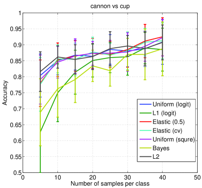
(a) Accuracy averaged over 20 train/test splits
Refer to caption
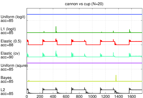
(b) Obtained kernel weights
Figure 1: Canon vs Cup from Caltech 101 dataset.
Refer to caption
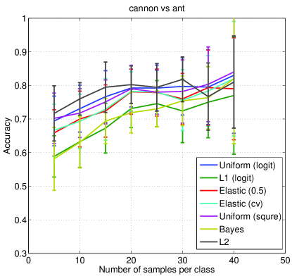
(a) Accuracy averaged over 20 train/test splits
Refer to caption
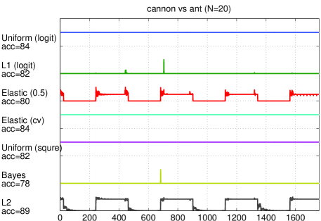
(b) Obtained kernel weights
Figure 2: Cannon vs Ant from Caltech 101 dataset.

Refer to caption
(a) Accuracy averaged over 20 train/test splits
Refer to caption
(b) Obtained kernel weights
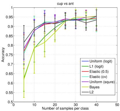
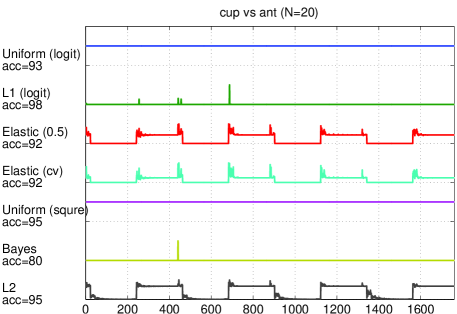
Figure 3: Cup vs Ant from Caltech 101 dataset.

Figures 13 show the results of applying different MKL algorithms. We can see that overall 2subscript2\ell_{2}-norm MKL, Elastic-net MKL, and uniformly-weighted MKL perform favorable compared to other MKL methods. Empirical Bayesian MKL and block 1-norm MKL tend to perform worse than the above three methods, especially when the number of samples per class is smaller than 20. However, in Figure 3, they do perform comparably for the number of samples per class above 30. Although Elastic-net MKL and 2subscript2\ell_{2}-norm MKL perform almost the same as uniform MKL in terms of accuracy, the right panels show that these methods can find important kernel components automatically. More specifically, on the “Cannon vs Cup” dataset (Figure 1), Elastic-net MKL chose 88 Gaussian RBF kernel functions and 792 χ2superscript𝜒2\chi^{2} kernel functions. Thus it prefers χ2superscript𝜒2\chi^{2} kernels to Gaussian RBF kernels. This agrees with the common choice in computer vision literature. In addition, Elastic-net MKL consistently chose the band width parameter γ=0.1𝛾0.1\gamma=0.1 for the Gaussian RBF kernels but it never chose γ=0.1𝛾0.1\gamma=0.1 for the χ2superscript𝜒2\chi^{2} kernels; instead it averaged all χ2superscript𝜒2\chi^{2} kernels from γ=1.2𝛾1.2\gamma=1.2 to γ=10𝛾10\gamma=10.

5 Conclusion

We have shown that various MKL and structured sparsity models including psubscript𝑝\ell_{p}-norm MKL, Elastic-net MKL, multi-task learning, Wedge penalty, and overlapped group lasso can be seen as applications of different regularization strategies. These models have been conventionally presented in either kernel-weight-based regularization or block-norm-based regularization. We have shown that these two formulations can be systematically mapped to each other under some conditions through a concave conjugate transformation; see Table 1.

Furthermore, we have proposed a marginal-likelihood-based kernel learning algorithm. We have shown that the propose empirical Bayesian MKL can be considered to be employing a nonconvex nonseparable regularizer on the kernel weights. Furthermore, we have derived the expression for the block-norm regularizer corresponding to the proposed empirical Bayesian MKL.

We have tested the classification performance as well as the resulting kernel weights of various regularized MKL models we have discussed on visual categorization task from Caltech 101 dataset using 1,760 kernels. We have shown that Elastic-net MKL can achieve comparable classification accuracy to uniform kernel combination with roughly half of the candidate kernels and provide information about the usefulness of the candidate kernels. 2subscript2\ell_{2}-norm MKL also achieves similar classification performance and qualitatively similar kernel weights. However 2subscript2\ell_{2}-norm MKL does not achieve sparsity in the kernel weights in contrast to Elastic-net MKL. Empirical Bayesian MKL tends to perform worse than the above two methods probably because the kernel weights it obtains becomes extremely sparse. One way to avoid such solution is to introduce hyper-priors for the kernel weights as in Urtasun (2010).

We are currently aiming to relax the sufficient condition in Theorem 1 to guarantee mapping from the kernel-weight-based formulation to block-norm-based formulation. We would also like to have a finer characterization of the block-norm regularizer corresponding to the empirical Bayesian MKL (see also Wipf and Nagarajan (2008)). Theoretical argument concerning when to use sparse MKL models (e.g., 1subscript1\ell_{1}-norm MKL or empirical Bayesian MKL) and when to use non-sparse MKL models (psubscript𝑝\ell_{p}-norm MKL) is also necessary.

Acknowledgement

We would like to thank Hisashi Kashima and Shinichi Nakajima for helpful discussions. This work was partially supported by MEXT Kakenhi 22700138, 22700289, and NTT Communication Science Laboratories.

References

  • Aflalo et al. (2009) J. Aflalo, A. Ben-Tal, C. Bhattacharyya, J. S. Nath, and S. Raman. Variable sparsity kernel learning — algorithms and applications. J. Mach. Learn. Res. (submitted), 2009.
  • Archambeau and Bach (2010) C. Archambeau and F. Bach. Multiple gaussian process models. In NIPS 2010 Workshop: New Directions in Multiple Kernel Learning, 2010.
  • Argyriou et al. (2008) A. Argyriou, T. Evgeniou, and M. Pontil. Convex multi-task feature learning. Machine Learning, 73(3):243–272, 2008. ISSN 0885-6125.
  • Aronszajn (1950) N. Aronszajn. Theory of reproducing kernels. Transactions of the American Mathematical Society, 68:337–404, 1950.
  • Bach et al. (2004) F. Bach, G. Lanckriet, and M. Jordan. Multiple kernel learning, conic duality, and the SMO algorithm. In the 21st International Conference on Machine Learning, pages 41–48, 2004.
  • Bach et al. (2005) F. R. Bach, R. Thibaux, and M. I. Jordan. Computing regularization paths for learning multiple kernels. In Advances in Neural Information Processing Systems 17, pages 73–80. MIT Press, 2005.
  • Boyd and Vandenberghe (2004) S. Boyd and L. Vandenberghe. Convex Optimization. Cambridge University Press, Cambridge, 2004.
  • Cortes et al. (2009) C. Cortes, M. Mohri, and A. Rostamizadeh. L2subscript𝐿2L_{2} regularization for learning kernels. In the 25th Conference on Uncertainty in Artificial Intelligence (UAI 2009), 2009. Montréal, Canada.
  • Damoulas and Girolami (2008) T. Damoulas and M. A. Girolami. Probabilistic multi-class multi-kernel learning: on protein fold recognition and remote homology detection. Bioinformatics, 24(10):1264–1270, 2008.
  • Evgeniou and Pontil (2004) T. Evgeniou and M. Pontil. Regularized multi–task learning. In Proceedings of the tenth ACM SIGKDD international conference on Knowledge discovery and data mining, pages 109–117. ACM, 2004. ISBN 1581138881.
  • Evgeniou et al. (2005) T. Evgeniou, C.A. Micchelli, and M. Pontil. Learning multiple tasks with kernel methods. Journal of Machine Learning Research, 6:615–637, 2005.
  • Fei-Fei et al. (2004) L. Fei-Fei, R. Fergus, and P. Perona. Learning generative visual models from few training examples: an incremental bayesian approach tested on 101 object categories. In IEEE. CVPR 2004 Workshop on Generative-Model Based Vision, 2004.
  • Gehler and Nowozin (2009) P. Gehler and S. Nowozin. Let the kernel figure it out; principled learning of pre-processing for kernel classifiers. In IEEE CVPR 2009, 2009.
  • Girolami and Rogers (2005) M. Girolami and S. Rogers. Hierarchic bayesian models for kernel learning. In Proceedings of the 22nd International Conference on Machine Learning, pages 241–248. ACM, 2005.
  • Grauman and Darrell (2007) K. Grauman and T. Darrell. The pyramid match kernel: Efficient learning with sets of features. JMLR, 8:725–760, 2007.
  • Huang et al. (2009) J. Huang, T. Zhang, and D. Metaxas. Learning with structured sparsity. In Proceedings of the 26th Annual International Conference on Machine Learning, pages 417–424. ACM, 2009.
  • Jacob et al. (2009) L. Jacob, G. Obozinski, and J.P. Vert. Group Lasso with overlap and graph Lasso. In Proceedings of the 26th Annual International Conference on Machine Learning, pages 433–440. ACM, 2009.
  • Jenatton et al. (2009) R. Jenatton, J.Y. Audibert, and F. Bach. Structured variable selection with sparsity-inducing norms. Technical report, arXiv:0904.3523, 2009.
  • Kloft et al. (2008) M. Kloft, U. Brefeld, P. Laskov, and S. Sonnenburg. Non-sparse multiple kernel learning. In NIPS 2008 Workshop on Kernel Learning: Automatic Selection of Optimal Kernels, Whistler, 2008.
  • Kloft et al. (2009) M. Kloft, U. Brefeld, S. Sonnenburg, P. Laskov, K.-R. Müller, and A. Zien. Efficient and accurate lp-norm multiple kernel learning. In Y. Bengio, D. Schuurmans, J. Lafferty, C. K. I. Williams, and A. Culotta, editors, Advances in Neural Information Processing Systems 22, pages 997–1005. 2009.
  • Kloft et al. (2010) M. Kloft, U. Rückert, and P. L. Bartlett. A unifying view of multiple kernel learning. In Proc. ECML 2010, 2010.
  • Lanckriet et al. (2004) G. Lanckriet, N. Cristianini, L. El Ghaoui, P. Bartlett, and M. Jordan. Learning the kernel matrix with semi-definite programming. Journal of Machine Learning Research, 5:27–72, 2004.
  • Lazebnik et al. (2006) S. Lazebnik, C. Schmid, and J. Ponce. Beyond bags of features: Spatial pyramid matching for recognizing natural scene categories. In Proc. IEEE CVPR, volume 2, pages 2169–2178, 2006.
  • Longworth and Gales (2009) C. Longworth and MJF Gales. Combining derivative and parametric kernels for speaker verification. IEEE Transactions on Audio, Speech, and Language Processing, 17(4):748–757, 2009.
  • MacKay (1992) D. J. C. MacKay. Bayesian interpolation. Neural computation, 4(3):415–447, 1992.
  • Micchelli and Pontil (2005) C. A. Micchelli and M. Pontil. Learning the kernel function via regularization. Journal of Machine Learning Research, 6:1099–1125, 2005.
  • Micchelli et al. (2010) Charles Micchelli, Jean Morales, and Massi Pontil. A family of penalty functions for structured sparsity. In J. Lafferty, C. K. I. Williams, J. Shawe-Taylor, R.S. Zemel, and A. Culotta, editors, Advances in Neural Information Processing Systems 23, pages 1612–1623. 2010.
  • Rasmussen and Williams (2006) C. E. Rasmussen and C. K. I. Williams. Gaussian Processes for Machine Learning. MIT Press, 2006.
  • Seeger and Nickisch (2008) M. Seeger and H. Nickisch. Large scale variational inference and experimental design for sparse generalized linear models. Technical report, arXiv:0810.0901, 2008.
  • Shawe-Taylor (2008) J. Shawe-Taylor. Kernel learning for novelty detection. In NIPS 08 Workshop: Kernel Learning – Automatic Selection of Optimal Kernels, 2008.
  • Sonnenburg et al. (2010) S. Sonnenburg, G. Rätsch, S. Henschel, C. Widmer, J. Behr, A. Zien, F. de Bona, A. Binder, C. Gehl, and V. Franc. The shogun machine learning toolbox. Journal of Machine Learning Research, 11:1799–1802, 2010.
  • Suzuki and Tomioka (2009) T. Suzuki and R. Tomioka. SpicyMKL. Technical report, arXiv:0909.5026, 2009.
  • Tipping (2001) M. E. Tipping. Sparse bayesian learning and the relevance vector machine. J. Mach. Learn. Res., 1:211–244, 2001.
  • Tomioka and Suzuki (2010) R. Tomioka and T. Suzuki. Sparsity-accuracy trade-off in MKL. Technical report, arXiv:1001.2615, 2010.
  • Urtasun (2010) R. Urtasun. A Gaussian process view on MKL. In NIPS 2010 Workshop: New Directions in Multiple Kernel Learning, 2010.
  • van de Sande et al. (2010) K. E. A. van de Sande, T. Gevers, and C. G. M. Snoek. Evaluating color descriptors for object and scene recognition. IEEE Transactions on Pattern Analysis and Machine Intelligence, 32(9):1582–1596, 2010.
  • Varma and Ray (2007) M. Varma and D. Ray. Learning the discriminative power-invariance trade-off. In IEEE 11th International Conference on Computer Vision (ICCV), pages 1–8. 2007.
  • Wipf and Nagarajan (2008) D. Wipf and S. Nagarajan. A new view of automatic relevance determination. In Advances in NIPS 20, pages 1625–1632. MIT Press, 2008.
  • Wipf and Nagarajan (2009) D. Wipf and S. Nagarajan. A unified bayesian framework for meg/eeg source imaging. NeuroImage, 44(3):947–966, 2009.
  • Yuan and Lin (2006) M. Yuan and Y. Lin. Model selection and estimation in regression with grouped variables. Journal of The Royal Statistical Society Series B, 68(1):49–67, 2006.
  • Zhang et al. (2004) Z. Zhang, D.Y. Yeung, and J.T. Kwok. Bayesian inference for transductive learning of kernel matrix using the tanner-wong data augmentation algorithm. In Proceedings of the Twenty-First International Conference on Machine Learning, page 118. ACM, 2004.
  • Zien and Ong (2007) A. Zien and C.S. Ong. Multiclass multiple kernel learning. In Proceedings of the 24th international conference on machine learning, pages 11910–1198. ACM, 2007.

A Proof of Equation (1) in a finite dimensional case

In this section, we provide a proof of Equation (1) when 1,,msubscript1subscript𝑚{\mathcal{H}}_{1},\ldots,{\mathcal{H}}_{m} are all finite dimensional. We assume that the input space 𝒳𝒳{\mathcal{X}} consists of N𝑁N points x1,,xNsubscript𝑥1subscript𝑥𝑁x_{1},\ldots,x_{N}, for example the training points. The function fmmsubscript𝑓𝑚subscript𝑚f_{m}\in{\mathcal{H}}_{m} is completely specified by the function values at the N𝑁N-points 𝒇m=(fm(x1),,fm(xN))subscript𝒇𝑚superscriptsubscript𝑓𝑚subscript𝑥1subscript𝑓𝑚subscript𝑥𝑁top\boldsymbol{f}_{m}=(f_{m}(x_{1}),\ldots,f_{m}(x_{N}))^{\top}. The kernel function kmsubscript𝑘𝑚k_{m} is also specified by the Gram matrix 𝑲m=(km(xi,xj))i,j=1Nsubscript𝑲𝑚superscriptsubscriptsubscript𝑘𝑚subscript𝑥𝑖subscript𝑥𝑗𝑖𝑗1𝑁\boldsymbol{K}_{m}=(k_{m}(x_{i},x_{j}))_{i,j=1}^{N}. The inner product fm,gmmsubscriptsubscript𝑓𝑚subscript𝑔𝑚subscript𝑚\left\langle f_{m},g_{m}\right\rangle_{{\mathcal{H}}_{m}} is written as fm,gmm=𝒇m𝑲m1𝒈msubscriptsubscript𝑓𝑚subscript𝑔𝑚subscript𝑚superscriptsubscript𝒇𝑚topsuperscriptsubscript𝑲𝑚1subscript𝒈𝑚\left\langle f_{m},g_{m}\right\rangle_{{\mathcal{H}}_{m}}=\boldsymbol{f}_{m}^{\top}\boldsymbol{K}_{m}^{-1}\boldsymbol{g}_{m}, where 𝒈msubscript𝒈𝑚\boldsymbol{g}_{m} is the N𝑁N-dimensional vector representation of gmmsubscript𝑔𝑚subscript𝑚g_{m}\in{\mathcal{H}}_{m}, assuming that the Gram matrix 𝑲msubscript𝑲𝑚\boldsymbol{K}_{m} is positive definite. It is easy to check the reproducibility; in fact, fm,km(,xi)=𝒇m𝑲m1𝑲m(:,i)=f(xi)subscript𝑓𝑚subscript𝑘𝑚subscript𝑥𝑖superscriptsubscript𝒇𝑚topsuperscriptsubscript𝑲𝑚1subscript𝑲𝑚:𝑖𝑓subscript𝑥𝑖\left\langle f_{m},k_{m}(\cdot,x_{i})\right\rangle=\boldsymbol{f}_{m}^{\top}\boldsymbol{K}_{m}^{-1}\boldsymbol{K}_{m}(:,i)=f(x_{i}), where 𝑲m(:,i)subscript𝑲𝑚:𝑖\boldsymbol{K}_{m}(:,i) is a column vector of the Gram matrix 𝑲msubscript𝑲𝑚\boldsymbol{K}_{m} that corresponds to the i𝑖ith sample point xisubscript𝑥𝑖x_{i}.

The right-hand side of Equation (1) is written as follows:

min𝒇1,,𝒇MNsubscriptsubscript𝒇1subscript𝒇𝑀superscript𝑁\displaystyle\min_{\boldsymbol{f}_{1},\ldots,\boldsymbol{f}_{M}\in{\mathbb{R}}^{N}} m=1M𝒇m𝑲m1𝒇mdms.t.m=1M𝒇m=𝒇¯.\displaystyle\sum_{m=1}^{M}\frac{\boldsymbol{f}_{m}^{\top}\boldsymbol{K}_{m}^{-1}\boldsymbol{f}_{m}}{d_{m}}\quad{\rm s.t.}\quad\sum_{m=1}^{M}\boldsymbol{f}_{m}=\bar{\boldsymbol{f}}.

Forming the Lagrangian, we have

m=1M𝒇m𝑲m1𝒇mdmsuperscriptsubscript𝑚1𝑀superscriptsubscript𝒇𝑚topsuperscriptsubscript𝑲𝑚1subscript𝒇𝑚subscript𝑑𝑚\displaystyle\sum_{m=1}^{M}\frac{\boldsymbol{f}_{m}^{\top}\boldsymbol{K}_{m}^{-1}\boldsymbol{f}_{m}}{d_{m}}
=m=1M𝒇m𝑲m1𝒇mdm+2𝜶(𝒇¯m=1M𝒇m)absentsuperscriptsubscript𝑚1𝑀superscriptsubscript𝒇𝑚topsuperscriptsubscript𝑲𝑚1subscript𝒇𝑚subscript𝑑𝑚2superscript𝜶top¯𝒇superscriptsubscript𝑚1𝑀subscript𝒇𝑚\displaystyle=\sum_{m=1}^{M}\frac{\boldsymbol{f}_{m}^{\top}\boldsymbol{K}_{m}^{-1}\boldsymbol{f}_{m}}{d_{m}}+2\boldsymbol{\alpha}^{\top}\!\!\left(\bar{\boldsymbol{f}}-\sum\nolimits_{m=1}^{M}\boldsymbol{f}_{m}\right)
𝜶(m=1Mdm𝑲m)𝜶+2𝜶𝒇¯absentsuperscript𝜶topsuperscriptsubscript𝑚1𝑀subscript𝑑𝑚subscript𝑲𝑚𝜶2superscript𝜶top¯𝒇\displaystyle\geq-\boldsymbol{\alpha}^{\top}\left(\sum\nolimits_{m=1}^{M}d_{m}\boldsymbol{K}_{m}\right)\boldsymbol{\alpha}+2\boldsymbol{\alpha}^{\top}\bar{\boldsymbol{f}}
max𝜶𝒇¯(m=1Mdm𝑲m)1𝒇¯,subscript𝜶absentsuperscript¯𝒇topsuperscriptsuperscriptsubscript𝑚1𝑀subscript𝑑𝑚subscript𝑲𝑚1¯𝒇\displaystyle\xrightarrow{\max_{\boldsymbol{\alpha}}}\bar{\boldsymbol{f}}^{\top}\left(\sum\nolimits_{m=1}^{M}d_{m}\boldsymbol{K}_{m}\right)^{-1}\bar{\boldsymbol{f}},

where the equality is obtained for

𝒇m=dm𝑲m(m=1Mdm𝑲m)1𝒇¯.subscript𝒇𝑚subscript𝑑𝑚subscript𝑲𝑚superscriptsuperscriptsubscript𝑚1𝑀subscript𝑑𝑚subscript𝑲𝑚1¯𝒇\boldsymbol{f}_{m}=d_{m}\boldsymbol{K}_{m}\left(\sum\nolimits_{m=1}^{M}d_{m}\boldsymbol{K}_{m}\right)^{-1}\bar{\boldsymbol{f}}.