Minimizing Communication for Eigenproblems and the Singular Value Decomposition

Abstract

Algorithms have two costs: arithmetic and communication. The latter represents the cost of moving data, either between levels of a memory hierarchy, or between processors over a network. Communication often dominates arithmetic and represents a rapidly increasing proportion of the total cost, so we seek algorithms that minimize communication. In [4] lower bounds were presented on the amount of communication required for essentially all $O(n^{3})$-like algorithms for linear algebra, including eigenvalue problems and the SVD. Conventional algorithms, including those currently implemented in (Sca)LAPACK, perform asymptotically more communication than these lower bounds require. In this paper we present parallel and sequential eigenvalue algorithms (for pencils, nonsymmetric matrices, and symmetric matrices) and SVD algorithms that do attain these lower bounds, and analyze their convergence and communication costs.

1 Introduction

The running time of an algorithm depends on two factors: the number of floating point operations executed (arithmetic) and the amount of data moved either between levels of a memory hierarchy in the case of sequential computing, or over a network connecting processors in the case of parallel computing (communication). The simplest metric of communication is to count the total number of words moved (also called the bandwidth cost). Another simple metric is to count the number of messages containing these words (also known as the latency cost). On current hardware the cost of moving a single word, or that of sending a single message, already greatly exceed the cost of one arithmetic operation, and technology trends indicate that this processor-memory gap is growing exponentially over time. So it is of interest to devise algorithms that minimize communication, sometimes even at the price of doing more arithmetic.

In this paper we present sequential and parallel algorithms for finding eigendecompositions and SVDs of dense matrices, that do $O(n^{3})$ arithmetic operations, are numerically stable, and do asymptotically less communication than previous such algorithms.

In fact, these algorithms attain known communication lower bounds that apply to many $O(n^{3})$ algorithms in dense linear algebra. In the sequential case, when the $n$-by-$n$ input matrix does not fit in fast memory of size $M$, the number of words moved between fast (small) and slow (large) memory is $\Omega(n^{3}/\sqrt{M})$. In the case of $P$ parallel processors, where each processor has room in memory for $1/P$-th of the input matrix, the number of words moved between one processor and the others is $\Omega(n^{2}/\sqrt{P})$. These lower bounds were originally proven for sequential [30] and parallel [32] matrix multiplication, and extended to many other linear algebra algorithms in [4], including the first phase of conventional eigenvalue/SVD algorithms: reduction to Hessenberg, tridiagonal and bidiagonal forms.

Most of our algorithms, however, do not rely on reduction to these condensed forms; instead they rely on explicit QR factorization (which is also subject to these lower bounds). This raises the question as to whether there is a communication lower bound independent of algorithm for solving the eigenproblem. We provide a partial answer by reducing the QR decomposition of a particular block matrix to computing the Schur form of a similar matrix, so that sufficiently general lower bounds on QR decomposition could provide lower bounds for computing the Schur form.

We note that there are communication lower bounds not just for the bandwidth cost, but also for the latency cost. Some of our algorithms also attain these bounds.

In more detail, we present three kinds of communication-minimizing algorithms, randomized spectral divide-and-conquer, eigenvectors from Schur Form, and successive band reduction.

Randomized spectral divide-and-conquer applies to eigenvalue problems for regular pencils $A-\lambda B$, the nonsymmetric and symmetric eigenvalue problem of a single matrix, and the singular value decomposition (SVD) of a single matrix. For $A-\lambda B$ it computes the generalized Schur form, and for a single nonsymmetric matrix it computes the Schur form. For a symmetric problem or SVD, it computes the full decomposition. There is an extensive literature on such divide-and-conquer algorithms: the PRISM project algorithm [2, 6], the reduction of the symmetric eigenproblem to matrix multiplication by Yau and Lu [35], the matrix sign function algorithm originally formulated in [31, 40], and the inverse-free approach originally formulated in [26, 12, 36, 37, 38], which led to the version [3, 14] from which we start here. Our algorithms will minimize communication, both bandwidth cost and latency cost, in both the two-level sequential memory model and parallel model (asymptotically, up to polylog factors). Because there exist cache-oblivious sequential algorithms for matrix multiplication [24] and QR decomposition [23], we conjecture that it is possible to devise cache-oblivious versions of the randomized spectral divide-and-conquer algorithms, thereby minimizing communication costs between multiple levels of the memory hierarchy on a sequential machine.

In particular, we fix a limitation in [3] (also inherited by [14]) which needs to compute a rank-revealing factorization of a product of matrices $A^{-1}B$ without explicitly forming either $A^{-1}$ or $A^{-1}B$. The previous algorithm used column pivoting that depended only on $B$, not $A$; this cannot a priori guarantee a rank-revealing decomposition, as the improved version we present in this paper does. In fact, we show here how to compute a randomized rank-revealing decomposition of an arbitrary product $A_{1}^{\pm 1}\cdots A_{p}^{\pm 1}$ without any general products or inverses, which is of independent interest.

We also improve the old methods ([3], [14]) by providing a “high level” randomized strategy (explaining how to choose where to split the spectrum), in addition to the “basic splitting” method (explaining how to divide the spectrum once a choice has been made). We also provide a careful analysis of both “high level” and “basic splitting” strategies (Section 3), and illustrate the latter on a few numerical examples.

Additionally, unlike previous methods, we show how to deal effectively with clustered eigenvalues (by outputting a convex polygon, in the nonsymmetric case, or a small interval, in the symmetric one, where the eigenvalues lie), rather than assume that eigenvalues can be spread apart by scaling (as in [35]).

Given the (generalized) Schur form, our second algorithm computes the eigenvectors, minimizing communication by using a natural blocking scheme. Again, it works sequentially or in parallel, minimizing bandwidth cost and latency cost.

Though they minimize communication asymptotically, randomized spectral divide-and-conquer algorithms perform several times as much arithmetic as do conventional algorithms. For the case of regular pencils and the nonsymmetric eigenproblem, we know of no communication-minimizing algorithms that also do about the same number of floating point operations as conventional algorithms. But for the symmetric eigenproblem (or SVD), it is possible to compute just the eigenvalues (or singular values) with very little extra arithmetic, or the eigenvectors (or singular vectors) with just 2x the arithmetic cost for sufficiently large matrices (or 2.6x for somewhat smaller matrices) while minimizing bandwidth cost in the sequential case. Minimizing bandwidth costs of these algorithms in the parallel case and minimizing latency in either case are open problems. These algorithms are a special case of the class of successive band reduction algorithms introduced in [7, 8].

The rest of this paper is organized as follows. Section 2 discusses randomized rank-revealing decompositions. Section 3 uses these decompositions to implement randomized spectral divide-and-conquer algorithms. Section 4 presents lower and upper bounds on communication. Section 5 discusses computing eigenvectors from matrices in Schur form. Section 6 discusses successive band reduction. Finally, Section 7 draws conclusions and presents some open problems.

2 Randomized Rank-Revealing Decompositions

Let $A$ be an $n\times n$ matrix with singular values $\sigma_{1}\geq\sigma_{2}\geq\ldots\geq\sigma_{n}$, and assume that there is a “gap” in the singular values at level $k$, that is, $\sigma_{1}/\sigma_{k}=O(1)$, while $\sigma_{k}/\sigma_{k+1}\gg 1$.

Informally speaking, a decomposition of the form $A=URV$ is called rank revealing if the following conditions are fulfilled:

• $U$ and $V$ are orthogonal/unitary and $R=\left[\begin{array}[]{cc}R_{11}&R_{12}\\ O&R_{22}\end{array}\right]$ is upper triangular, with $R_{11}$ $k\times k$ and $R_{22}$ $(n-k)\times(n-k)$;

• $\sigma_{min}(R_{11})$ is a “good” approximation to $\sigma_{k}$ (at most a factor of a low-degree polynomial in $n$ away from it),

• $\sigma_{max}(R_{22})$ is a “good” approximation to $\sigma_{k+1}$ (at most a factor of a low-degree polynomial in $n$ away from it);

• In addition, if $||R_{11}^{-1}R_{12}||_{2}$ is small (at most a low-degree polynomial in $n$), then the rank-revealing factorization is called strong (as per [28]).

Rank revealing decompositions are used in rank determination [44], least square computations [13], condition estimation [5], etc., as well as in divide-and-conquer algorithms for eigenproblems. For a good survey paper, we recommend [28].

In the paper [14], we have proposed a randomized rank revealing factorization algorithm RURV. Given a matrix $A$, the routine computes a decomposition $A=URV$ with the property that $R$ is a rank-revealing matrix; the way it does it is by “scrambling” the columns of $A$ via right multiplication by a uniformly random orthogonal (or unitary) matrix $V^{H}$. The way to obtain such a random matrix (whose described distribution over the manifold of unitary/orthogonal matrices is known as Haar) is to start from a matrix $B$ of independent, identically distributed normal variables of mean $0$ and variance $1$, denoted here and throughout the paper by $N(0,1)$. The orthogonal/unitary matrix $V$ obtained from performing the QR algorithm on the matrix $B$ is Haar distributed.

Performing QR on the resulting matrix $AV^{H}=:\hat{A}=UR$ yields two matrices, $U$ (orthogonal or unitary) and $R$ (upper triangular), and it is immediate to check that $A=URV$.

Algorithm 1 Function $[U,R,V]=$RURV$(A)$, computes a randomized rank revealing decomposition $A=URV$, with $V$ a Haar matrix.

1:  Generate a random matrix $B$ with i.i.d. $N(0,1)$ entries.

2:  $[V,\hat{R}]=$QR$(B)$.

3:  $\hat{A}=A\cdot V^{H}$.

4:  $[U,R]=$ QR$(\hat{A})$.

5:  Output $R$.

It was proven in [14] that, with high probability, RURV computes a good rank revealing decomposition of $A$ in the case of $A$ real. Specifically, the quality of the rank-revealing decomposition depends on computing the asymptotics of $f_{r,n}$, the smallest singular value of an $r\times r$ submatrix of a Haar-distributed orthogonal $n\times n$ matrix. All the results of [14] can be extended verbatim to Haar-distributed unitary matrices; however, the analysis employed in [14] is not optimal. In [22], the asymptotically exact scaling and distribution of $f_{r,n}$ were computed for all regimes of growth $(r,n)$ (naturally, $0<r<n$). Essentially, the bounds state that $\sqrt{r(n-r)}f_{r,n}$ converges in law to a given distribution, both for the real and for the complex cases.

The result of [14] states that RURV is, with high probability, a rank-revealing factorization. Here we strengthen these results to argue that it if in fact a strong rank-revealing factorization, in the sense of [28], since with high probability $||R_{11}^{-1}R_{12}||$ will be small. We obtain the following theorem.

Theorem 2.1.

Let $A$ be an $n\times n$ matrix with singular values $\sigma_{1},\ldots,\sigma_{r},\sigma_{r+1},\ldots,\sigma_{n}$. Let $\epsilon>0$ be a small number. Let $R$ be the matrix produced by the RURV algorithm on $A$. Assume that $n$ is large and that $\frac{\sigma_{1}}{\sigma_{r}}=M$ and that $\frac{\sigma_{r}}{\sigma_{r+1}}>Cn$ for some constants $M$ and $C>1$, independent of $n$.

There exist constants $c_{1}$, $c_{2}$, and $c_{3}$ such that, with probability $1-O(\epsilon)$, the following three events occur:

$$c_{1}\frac{\sigma_{r}}{\sqrt{r(n-r)}} \leq \sigma_{\min}(R_{11})\leq\sqrt{2}\sigma_{r}~{},$$

$$\sigma_{r+1} \leq \sigma_{\max}(R_{22})\leq\left(3M^{3}\frac{C^{2}}{C^{2}-1}\right)\frac{r^{2}(n-r)^{2}\sigma_{r+1}}{c_{2}}~{},~{}~{}~{}\mbox{and}$$

$$||R_{11}^{-1}R_{12}||_{2} \leq c_{3}\sqrt{r(n-r)}~{}.$$

Proof.

There are two cases of the problem, $r\leq n/2$ and $r>n/2$. Let $V$ be the Haar matrix used by the algorithm. From Theorem 2.4-1 in [27], the singular values of $V(1;r,1:r)$ when $r>n/2$ consist of $(2r-n)$ $1$’s and the singular values of $V((r+1):n,(r+1):n)$. Thus, the case $r>n/2$ reduces to the case $r\leq n/2$.

The first two relationships follow immediately from [14] and [22]; the third we will prove here.

We use the following notation. Let $A=P\Sigma Q^{H}=P\cdot{\rm diag}(\Sigma_{1},\Sigma_{2})\cdot Q^{H}$ be the singular value decomposition of $A$, where $\Sigma_{1}={\rm diag}(\sigma_{1},\ldots,\sigma_{r})$ and $\Sigma_{2}={\rm diag}(\sigma_{r+1},\ldots,\sigma_{n})$. Let $V^{H}$ be the random unitary matrix in RURV. Then $X=Q^{H}V^{H}$ has the same distribution as $V^{H}$, by virtue of the fact that $V$’s distribution is uniform over unitary matrices.

Write

$$X=\left[\begin{array}[]{cc}X_{11}&X_{12}\\ X_{21}&X_{22}\end{array}\right]~{},$$

where $X_{11}$ is $r\times r$, and $X_{22}$ is $(n-r)\times(n-r)$.

Then

$$U^{H}P\cdot\Sigma X=R~{};$$

denote $\Sigma\cdot X=[Y_{1},Y_{2}]$ where $Y_{1}$ is an $n\times r$ matrix and $Y_{2}$ in an $(n-r)\times n$ one. Since $U^{H}P$ is unitary, in effect

$$R_{11}^{-1}R_{12}=Y_{1}^{+}Y_{2}~{},$$

where $Y_{1}^{+}$ is the pseudoinverse of $Y_{1}$, i.e. $Y_{1}^{+}=(Y_{1}^{H}Y_{1})^{-1}Y_{1}^{H}$. We obtain that

$$R_{11}^{-1}R_{12}=\left(X_{11}^{H}\Sigma^{2}X_{11}+X_{21}^{H}\sigma_{2}^{2}X_{21}\right)^{-1}\left(X_{11}^{H}\Sigma_{1}^{2}X_{12}+X_{21}^{H}\Sigma_{2}^{2}X_{22}\right)~{}.$$

Examine now

$$T_{1}:=\left(X_{11}^{H}\Sigma_{1}^{2}X_{11}+X_{21}^{H}\Sigma^{2}_{2}X_{21}\right)^{-1}X_{11}^{H}\Sigma_{1}^{2}X_{12}=X_{11}^{-1}\left(\Sigma_{1}^{2}+(X_{21}X_{11}^{-1})^{H}\Sigma_{2}^{2}(X_{21}X_{11}^{-1})\right)^{-1}\Sigma_{1}^{2}X_{12}~{}.$$

Since $X_{12}$ is a submatrix of a unitary matrix, $||X_{12}||\leq 1$, and thus

$$||T_{1}||\leq||X_{11}||^{-1}||I_{r}+\Sigma_{1}^{-2}(X_{21}X_{11}^{-1})^{H}\Sigma_{2}^{2}(X_{21}X_{11}^{-1})||^{-1}\leq\frac{1}{\sigma_{\min}(X_{11})}\cdot\frac{1}{1-\sigma_{r+1}^{2}\sigma_{\min}(X_{11})^{2}/\sigma_{r}^{2}}~{}.$$ (1)

Given that $\sigma_{\min}(X_{11})=O((\sqrt{r(n-r)})^{-1})$ with high probability and $\sigma_{r}/\sigma_{r+1}\geq Cn$, it follows that the denominator of the last fraction in (1) is $O(1)$. Therefore, there must exist a constant such that, with probability bigger than $1-\epsilon$, $||T_{1}||\leq c_{3}\sqrt{r(n-r)}$. Note that $c_{3}$ depends on $\epsilon$.

The same reasoning applies to the term

$$T_{2}:=\left(X_{11}^{H}\Sigma_{1}^{2}X_{11}+X_{21}^{H}\Sigma^{2}_{2}X_{21}\right)^{-1}X_{21}\Sigma_{2}^{2}X_{22}~{};$$

to yield that

$$||T_{2}||\leq||X_{11}^{-1}||^{2}||I_{r}+\Sigma_{1}^{-2}(X_{21}X_{11}^{-1})^{H}\Sigma_{2}^{2}(X_{21}X_{11}^{-1})||^{-1}||\Sigma_{1}^{-2}||\cdot||\Sigma_{2}^{2}||,$$ (2)

because $||X_{22}||\leq 1$.

The conditions imposed in the hypothesis ensure that $||X_{11}^{-1}||\cdot||\Sigma_{1}^{-1}||\cdot||\Sigma_{2}||=O(1)$, and thus $||T_{2}||=O(1)$.

From (1) and (2), the conclusion follows. $\Box$

The bounds on $\sigma_{\min}(R_{11})$ are as good as any deterministic algorithm would provide (see [28]). However, the upper bound on $\sigma_{\max}(R_{22})$ is much weaker than in corresponding deterministic algorithms. We suspect that this may be due to the fact that the methods of analysis are too lax, and that it is not intrinsic to the algorithm.

This theoretical sub-optimality will not affect the performance of the algorithm in practice, as it will be used to differentiate between singular values $\sigma_{r+1}$ that are very small (polynomially close to $0$) and singular values $\sigma_{r}$ that are close to $1$, and thus far enough apart.

Similarly to RURV we define the routine RULV, which performs the same kind of computation (and obtains a rank revealing decomposition of $A$), but uses QL instead of QR, and thus obtains a lower triangular matrix in the middle, rather than an upper triangular one.

Given RURV and RULV, we now can give a method to find a randomized rank-revealing factorization for a product of matrices and inverses of matrices, without actually computing any of the inverses or matrix products. This is a very interesting and useful procedure in itself, but we will also use it in Sections 3 and 3.2 in the analysis of a single step of our Divide-and-Conquer algorithms.

Suppose we wish to find a randomized rank-revealing factorization $M_{k}=URV$ for the matrix $M_{k}=A_{1}^{m_{1}}\cdot A_{2}^{m_{2}}\cdot\ldots A_{k}^{m_{k}}$, where $A_{1},\ldots,A_{k}$ are given matrices, and $m_{1},\ldots,m_{k}\in\{-1,1\}$, without actually computing $M_{k}$ or any of the inverses.

Essentially, the method performs RURV or, depending on the power, RULV, on the last matrix of the product, and then uses a series of QR/RQ to “propagate” an orthogonal/unitary matrix to the front of the product, while computing factor matrices from which (if desired) the upper triangular $R$ matrix can be obtained. A similar idea was explored by G.W. Stewart in [45] to perform graded QR; although it was suggested that such techniques can be also applied to algorithms like URV, no randomization was used.

The algorithm is presented in pseudocode below.

Algorithm 2 Function $U=$GRURV$(k;A_{1},\ldots,A_{k};m_{1},\ldots,m_{k})$, computes the $U$ factor in a randomized rank revealing decomposition of the product matrix $M_{k}=A_{1}^{m_{1}}\cdot A_{2}^{m_{2}}\cdot\ldots A_{k}^{m_{k}}$, where $m_{1},\ldots,m_{k}\in\{-1,1\}$.

1:  if $m_{k}=1$, then

2:     $[U,R_{k},V]=\textbf{RURV}(A_{k})$

3:  else

4:     $[U,L_{k},V]=\textbf{RULV}(A_{k}^{H})$

5:     $R_{k}=L_{k}^{H}$

6:  end if

7:  $U_{current}=U$

8:  for $i=k-1$ downto $1$ do

9:     if $m_{i}=1$, then

10:        $[U,R_{i}]=\textbf{QR}(A_{i}\cdot U_{current})$

11:        $U_{current}=U$

12:     else

13:        $[U,R_{i}]=\textbf{RQ}(U_{current}^{H}\cdot A_{i})$

14:        $U_{current}=U^{H}$

15:     end if

16:  end for

17:  return  $U_{current}$, optionally $V,R_{1},\ldots,R_{k}$

Lemma 2.2.

GRURV (Generalized Randomized URV) computes the rank-revealing decomposition $M_{k}=U_{current}R_{1}^{m_{1}}\ldots R_{k}^{m_{k}}V$.

Proof.

Let us examine the case when $k=2$ ($k>2$ results immediately through simple induction).

Let us examine the cases:

1. $m_{2}=1$. In this case, $M_{2}=A_{1}^{m_{1}}A_{2}$; the first RURV yields $M_{2}=A_{1}^{m_{1}}UR_{2}V$.

   1. if $m_{1}=1$, $M_{2}=A_{1}UR_{2}V$; performing QR on $A_{1}U$ yields $M_{2}=U_{current}R_{1}R_{2}V$.

   2. if $m_{1}=-1$, $M_{2}=A_{1}^{-1}UR_{2}V$; performing RQ on $U^{H}A_{1}$ yields $M_{2}=U_{current}R_{1}^{-1}R_{2}V$.

2. $m_{2}=-1$. In this case, $M_{2}=A_{1}^{m_{1}}A_{2}^{-1}$; the first RULV yields $M_{2}=A_{1}^{m_{1}}UL_{2}^{-H}V=A_{1}^{m_{1}}UR_{2}^{-1}V$.

   1. if $m_{1}=1$, $M_{2}=A_{1}UL_{2}^{-H}V=A_{1}UR_{2}^{-1}V$; performing QR on $A_{1}U$ yields $M_{2}=U_{current}R_{1}R_{2}^{-1}V$.

   2. finally, if $m_{2}=-1$, $M_{2}=A_{1}^{-1}UL_{2}^{-H}V=A_{1}^{-1}UR_{2}^{-1}V$; performing RQ on $U^{H}A_{1}$ yields $M_{2}=U_{current}R_{1}^{-1}R_{2}^{-1}V$.

Note now that in all cases $M_{k}=U_{current}R_{1}^{m_{1}}\ldots R_{k}^{m_{k}}V$. Since the inverse of an upper triangular matrix is upper triangular, and since the product of two upper triangular matrices is upper triangular, it follows that $R:=R_{1}^{m_{1}}\ldots R_{k}^{m_{k}}$ is upper triangular. Thus, we have obtained a rank-revealing decomposition of $M_{k}$; the same rank-revealing decomposition as if we have performed $QR$ on $M_{k}V^{H}$. $\Box$

By using the stable QR and RQ algorithms described in [14], as well as RURV, we can guarantee the following result.

Theorem 2.3.

The result of the algorithm GRURV is the same as the result of RURV on the (explicitly formed) matrix $M_{k}$; therefore, given a large gap in the singular values of $M_{k}$, $\sigma_{r+1}\ll\sigma_{r}\sim\sigma_{1}$, the algorithm GRURV produces a rank-revealing decomposition with high probability.

Note that we may also return the matrices $R_{1},\ldots,R_{k}$, from which the factor $R$ can later be reassembled, if desired (our algorithms only need $U_{current}$, not $R=R_{1}^{m_{1}}\ldots R_{k}^{m_{k}}$, and so we will not compute it).

3 Divide-and-Conquer: Four Versions

As mentioned in the Introduction, the idea for the divide-and-conquer algorithm we propose has been first introduced in [36]; it was subsequently made stable in [3], and has then been modified in [14] to include a randomized rank-revealing decomposition, in order to minimize the complexity of linear algebra (reducing it to the complexity of matrix multiplication, while keeping algorithms stable). The version of RURV presented in this paper is the only complete one, through the introduction of GRURV; also, the new analysis shows that it has stronger rank-revealing properties than previously shown.

Since in [14] we only sketched the merger of the rank-revealing decomposition and the eigenvalue/singular value decomposition algorithms, we present the full version in this section, as it will be needed to analyze communication. We give the most general version RGNEP (which solves the generalized, non-symmetric eigenvalue problem), as well as versions RNEP (for the non-symmetric eigenvalue problem), RSEP (for the symmetric eigenvalue problem), and RSVD (for the singular value problem). The acronyms here are the same used in LAPACK, with the exception of the first letter “R”, which stands for “randomized”.

In this section and throughout the rest of the paper, QR, RQ, QL, and LQ represent functions/routines computing the corresponding factorizations. Although these factorizations are well-known, the implementations of the routines are not the “standard” ones, but the communication-avoiding ones described in [4]. We only consider the latter, for the purpose of minimizing communication.

3.1 Basic splitting algorithms (one step)

Let $\mathcal{D}$ be the interior of the unit disk. Let $A$, $B$ be two $n\times n$ matrices with the property that the pencil $(A,B)$ has no eigenvalues on $\mathcal{D}$. The algorithm below “splits” the eigenvalues of the pencil $(A,B)$ into two sets; the ones inside $\mathcal{D}$ and the ones outside $\mathcal{D}$.

The method is as follows:

1. Compute $(I+(A^{-1}B)^{2^{k}})^{-1}$ implicitly. Roughly speaking, this maps the eigenvalues inside the unit circle to $0$ and those outside to $1$.

2. Compute a rank-revealing decomposition to find the right deflating subspace corresponding to eigenvalues inside the unit circle. This is spanned by the leading columns of a unitary matrix $Q_{R}$.

3. Analogously compute $Q_{L}$ from $(I+(A^{-H}B^{H})^{2^{k}})^{-1}$.

4. Output the block-triangular matrices

   $$\hat{A}=Q_{L}^{H}AQ_{R}=\left(\begin{array}[]{cc}A_{11}&A_{12}\\ E_{21}&A_{22}\end{array}\right)~{},~{}~{}~{}~{}~{}\hat{B}=Q_{L}^{H}BQ_{R}=\left(\begin{array}[]{cc}B_{11}&B_{12}\\ F_{21}&B_{22}\end{array}\right)~{}.$$

The pencil $(A_{11},B_{11})$ has no eigenvalues inside $\mathcal{D}$; the pencil $(A_{22},B_{22})$ has no eigenvalues outside $\mathcal{D}$. In exact arithmetic and after complete convergence, we should have $E_{21}=F_{21}=0$. In the presence of floating point error with a finite number of iterations, we use $||E_{21}||_{1}/||A||_{1}$ and $||F_{21}||_{1}/||B||_{1}$ to measure the stability of the computation.

To simplify the main codes, we first write a routine to perform (implicitly) repeated squaring of the quantity $A^{-1}B$. The proofs for correctness are in the next section.

Algorithm 3 Function IRS, performs implicit repeated squaring of the quantity $A^{-1}B$ for a pair of matrices $(A,B)$

1:  Let $A_{0}=A$ and $B_{0}=B$; j = 0.

2:  repeat

3:     

$$\left(\begin{array}[]{c}B_{j}\\ -A_{j}\end{array}\right) = \left(\begin{array}[]{cc}Q_{11}&Q_{12}\\ Q_{21}&Q_{22}\end{array}\right)\left(\begin{array}[]{c}R_{j}\\ 0\end{array}\right)~{},$$

$$A_{j+1} = Q^{H}_{12}A_{j}~{},$$

$$B_{j+1} = Q^{H}_{22}B_{j}~{},$$

4:     if $||R_{j}-R_{j-1}||_{1}\leq\tau||R_{j-1}||_{1}~{},$                            … convergence!  then

5:        $p=j+1~{},$

6:     else

7:        $j=j+1$

8:     end if

9:  until convergence or $j>maxit$.

10:  return  $A_{p}$, $B_{p}$.

Armed with repeated squaring, we can now perform a step of divide-and-conquer. We start with the most general case of a two-matrix pencil.

Algorithm 4 Function RGNEP, performs a step of divide-and-conquer on a pair of matrices $A$ and $B$

1:  $[A_{p},B_{p}]=$IRS$(A,B)$.

2:  $Q_{R}=$GRURV$(2,A_{p}+B_{p},A_{p},-1,1)$.

3:  $[A_{p},B_{p}]=$IRS$(A^{H},B^{H})$.

4:  $Q_{L}=$GRURV$(2,A_{P}^{H},(A_{p}+B_{p})^{H},1,-1)$.

5:  

$$\hat{A} := Q_{L}^{H}AQ_{R}=\left(\begin{array}[]{cc}A_{11}&A_{12}\\ E_{21}&A_{22}\end{array}\right)~{},$$ (6)

$$\hat{B} := Q_{L}^{H}BQ_{R}=\left(\begin{array}[]{cc}B_{11}&B_{12}\\ F_{21}&B_{22}\end{array}\right)~{};$$ (9)

the dimensions of the subblocks are chosen so as to minimize $||E_{21}||_{1}/||A||_{1}+||F_{21}||_{1}/||B||_{1}$;

6:  return  $(\hat{A},\hat{B},Q_{L},Q_{R})$ and the dimensions of the subblocks.

The algorithm RGNEP starts with the right deflating subspace: line 1 does implicit repeated squaring of $A^{-1}B$, followed by a rank-revealing decomposition of $(A_{p}+B_{p})^{-1}A_{p}$ (line 2). The left deflating subspace is handled similarly in lines 3 and 4. Finally, line 5 divides the pencil by choosing the split that minimizes the sum of the relative norms of the bottom-left submatrices, e.g. $||E_{21}||_{1}/||A||_{1}+||F_{21}||_{1}/||B||_{1}$. If this norm is small enough, convergence is successful. In this case $E_{21}$ and $F_{21}$ may be zeroed out, dividing the problem into two smaller ones, given by $(A_{11},B_{11})$ and $(A_{22},B_{22})$. Note that if more than one pair of blocks $(E_{21},F_{21})$ is small enough to zero out, the problem may be divided into more than two smaller ones.

Algorithm 5 Function RNEP, performs a step of divide-and-conquer on a non-hermitian matrix $A$; $I$ here is the identity matrix.

1:  $[A_{p},B_{p}]=$IRS$(A,I)$.

2:  $Q=$GRURV$(2,A_{p}+B_{p},A_{p},-1,1)$.

3:  

$$\hat{A} := Q^{H}AQ=\left(\begin{array}[]{cc}A_{11}&A_{12}\\ E_{21}&A_{22}\end{array}\right)~{},$$

the dimensions of the subblocks are chosen so as to minimize $||E_{21}||_{1}/||A||_{1}$;

4:  return  $(\hat{A},Q)$ and the dimensions of the blocks.

The algorithm RNEP deals with the non-symmetric eigenvalue problem, that is, when $A$ is non-hermitian and $B=I$. In this case, we skip the computation of the left deflating subspace, since it is the same as the right one; also, it is sufficient to consider $||E_{21}||_{1}/||A||_{1}$, since it is the backward error in the computation. Note that (9) is not needed, as in exact arithmetic $\hat{B}=I$.

Algorithm 6 Function RSEP, performs a step of divide-and-conquer on a hermitian matrix $A$; $I$ here is the identity matrix.

1:  $[A_{p},B_{p}]=$IRS$(A,I)$.

2:  $[U,R_{1},V]=$GRURV$(2,A_{p}+B_{p},A_{p},-1,1)$.

3:  

$$\hat{A} := Q^{H}AQ$$

$$\hat{A} := \frac{\hat{A}+\hat{A}^{H}}{2}$$

$$\hat{A} := \left(\begin{array}[]{cc}A_{11}&E_{21}^{T}\\ E_{21}&A_{22}\end{array}\right)~{},$$

the dimensions of the subblocks are chosen so as to minimize $||E_{21}||_{1}/||A||_{1}$;

4:  return  $(\hat{A},Q)$ and the dimensions of the blocks.

The algorithm RSEP is virtually identical to RNEP, with the only difference in the second equation of line 3, where we enforce the symmetry of $\hat{A}$. We choose to write two separate pieces of code for RSEP and RNEP, as the analysis of theses two codes in Section 3.2 differs.

We choose to explain the routine for computing singular values of a matrix $A$, rather than present it in pseudocode. Instead of calculating the singular values of $A$ directly, we construct the hermitian matrix $B=\left[\begin{array}[]{cc}0&A\\ A^{H}&0\end{array}\right]$ and compute its eigenvalues (which are the singular values of $A$ and their negatives) and eigenvectors (which are concatenations of left and right singular vectors of $A$). Thus, computing singular values completely reduces to computing eigenvalues.

3.2 One step: correctness and reliability of implicit repeated squaring

Assume for simplicity that all matrices involved are invertible, and let us examine the basic step of the algorithm IRS. It is easy to see that

$$\left(\begin{array}[]{cc}Q_{11}^{H}&Q_{21}^{H}\\ Q_{12}^{H}&Q_{22}^{H}\end{array}\right)\left(\begin{array}[]{c}B_{j}\\ -A_{j}\end{array}\right)=\left(\begin{array}[]{c}Q_{11}^{H}B_{j}-Q_{21}^{H}A_{j}\\ Q_{12}^{H}B_{j}-Q_{22}^{H}A_{j}\end{array}\right)=\left(\begin{array}[]{c}R_{j}\\ 0\end{array}\right)~{},$$

thus $Q_{12}^{H}B_{j}=Q_{22}^{H}A_{j}$, and then $B_{j}A_{j}^{-1}=Q_{12}^{-H}Q_{22}$; finally,

$$A_{j+1}^{-1}B_{j+1}=A_{j}^{-1}Q_{12}^{-H}Q_{22}^{H}B_{j}=(A_{j}^{-1}B_{j})^{2}~{},$$

proving that the algorithm IRS repeatedly squares the eigenvalues, sending those outside the unit circle to $\infty$, and the ones inside to $0$.

As in the proof of correctness from [3], we note that

$$(A_{p}+B_{p})^{-1}A_{p}=(I+A_{p}^{-1}B_{p})^{-1}=(I+(A^{-1}B)^{2^{p}})^{-1}~{},$$

and that the latter matrix approaches $P_{R,|z|>1}$, the projector onto the right deflating subspace corresponding to eigenvalues outside the unit circle.

3.3 High level strategy for divide-and-conquer, single non-symmetric matrix case

For the rest of this section, we will assume that the matrix $B=I$ and that the matrix $A$ is diagonalizable, with eigenvector matrix $S$ and spectral radius $\rho(A)$.

The first step will be to find (e.g., using Gershgorin bounds) a radius $R\geq\rho(A)$, so that we are assured that all eigenvalues are in the disk of radius $R$. Choose now a random angle $\theta$, uniformly from $[0,2\pi]$, and draw a radial line $\mathcal{R}$ through the origin, at angle $\theta$. The line $\mathcal{R}$ intersects the circle centered at the origin of radius $R/2$ at two points defining a diameter of the circle, $A$ and $B$. We choose a random point $a$ uniformly on the segment $AB$ and construct a line $\mathcal{L}$ perpendicular to $AB$ through $a$.

The idea behind this randomization procedure is to avoid not just “hitting” the eigenvalues, but also “hitting” some appropriate $\epsilon$-pseudospectrum of the matrix, defined below (the right choice for $\epsilon$ will be discussed later).

Definition 3.1.

(Following [46].) The $\epsilon$-pseudospectrum of a matrix $A$ is defined as

$$\Lambda_{\epsilon}(A)=\{z\in\mathbb{C}~{}|~{}z~{}\mbox{is an eigenvalue of}~{}A+E~{}\mbox{for some}~{}E~{}\mbox{with}~{}||E||_{2}\leq\epsilon\}$$

We measure progress in two ways: one is when a split occurs, i.e., we separate some part of the pseudospectrum, and the second one is when a large piece of the disk is determined not to contain any part of the pseudospectrum. This explains limiting the choice of $\mathcal{L}$ to only half the diameter of the circle; this way, we ensure that as long as we are not “hitting” the $\epsilon$-pseudospectrum, we are making progress. See Figure 1.

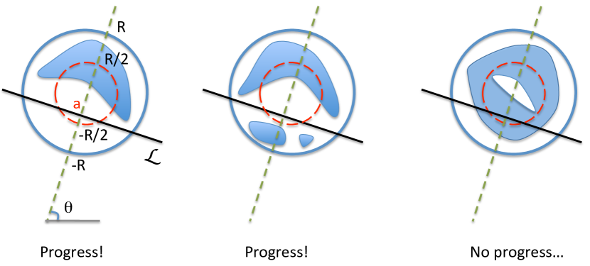
Figure 1: The possible outcomes of choosing a splitting line. The shaded shapes represent pseudospectral components, the dashed inner circle has radius $R/2$, the dashed line is at the random angle $\theta$, and the solid line is $\mathcal{L}$.

Remark 3.2.

It is thus possible that the ultimate answer could be a convex hull of the pseudospectrum; this is an alternative to the output that classical (or currently implemented) algorithms yield, which samples the pseudospectrum. Since in general pseudospectra can be arbitrarily complicated (see [39]), the amount of information gained may be limited; for example, the genus of the pseudospectrum will not be specified (i.e., the output will ignore the presence of “holes”, as in the third picture on Figure 1). However, in the case of convex or almost convex pseudospectra, a convex hull may be more informative than sampling.

Remark 3.3.

One could also imagine a method by which one could attempt to detect “holes” in the pseudospectrum, e.g., by sampling random points inside of the convex hull obtained and “fitting” disks centered at the points. Providing a detailed explanation for this case falls outside the scope of this paper.

Let us now compute a bound on the probability that the line $\mathcal{L}$ does not intersect a particular pseudospectrum of $A$ (which will depend on the machine precision, norm of $A$, etc.). To this extent, we will first examine the probability that the line $\mathcal{L}$ is at (geometrical) distance at least $\hat{\epsilon}$ from the spectrum of $A$.

Note that the problem is rotationally invariant; therefore it suffices to consider the case when $\theta=0$, and simply examine the case when $\mathcal{L}$ is $x=a$, i.e., our random line is a vertical line passing through the point $a$ on the segment $[-R/2,R/2]$.

Consider now the $n$ $\hat{\epsilon}$-balls that $\mathcal{L}$ must not intersect, and put a vertical “tube” around each one of them (as in Figure 2). These tubes will intersect the segment $[-R,R]$ in $n$ (possibly overlapping) small segments (of length $2\hat{\epsilon}$). In the worst-case scenario, they are all inside the segment $[-R/2,R/2]$, with no tubes overlapping. If the point $a$, chosen uniformly, falls into any one of them, the random line $\mathcal{L}$ will fall within $\hat{\epsilon}$ of the corresponding eigenvalue. This happens with probability at most $2\hat{\epsilon}n/R$.

The above argument proves the following lemma:

Lemma 3.4.

Let $d_{g}$ be the geometrical distance between the (randomly chosen) line $\mathcal{L}$ and the spectrum. Then

$$P[d_{g}\geq\hat{\epsilon}]\geq\max\{1-\frac{2n\hat{\epsilon}}{R}~{},0\}~{}.$$ (12)

Figure 2: Projecting the $\hat{\epsilon}$ tubes onto $[-R,R]$; the randomly chosen line $\mathcal{L}$ (i.e., $x=a$) does not intersect the (thick) projection segments (each of length $2\hat{\epsilon}$) with probability at least $1-\frac{2n\hat{\epsilon}}{R}$. The disks are centered at eigenvalues.

We would like now to estimate the number of iterations that the algorithm will need to converge, so we will use the results from [3]. To use them, we need to map the problem so that the splitting line becomes the unit circle. We will thus revisit the parameters that were essential in understanding the number of iterations in that case, and we will see how they change in the new context.

We start by recalling the notation $d_{(A,B)}$ for the “distance to the nearest ill-posed problem” (in our case, “ill-posed” means that there is an eigenvalue on the unit circle) for the matrix pencil $(A,B)$, defined as follows:

$$d_{(A,B)}\equiv\inf\{||E||+||F||~{}:(A+E)-z(B+F)~{}\mbox{is singular for some $z$ where $|z|=1$}\}~{};$$

according to Lemma 1, Section 5 from [3], $d_{(A,B)}=\min_{\theta}\sigma_{\min}(A-e^{i\theta}B)$.

We use now the estimate for the number $p$ of iterations given in Theorem 1 of Section 4 from [3]. Provided that the number of iterations, $p$, is larger than

$$p\geq\log_{2}\frac{||(A,B)||-d_{(A,B)}}{d_{(A,B)}}~{},$$ (13)

the relative distance between $(A_{p}+B_{p})^{-1}A_{p}$ and the projector $P_{R,|z|>1}$ may be bounded from above, as follows:

$$err_{p}:=\frac{||(A_{p}+B_{p})^{-1}A_{p}-P_{R,|z|>1}||}{||P_{R,|z|>1}||}\leq\frac{2^{p+3}\left(1-\frac{d_{(A,B)}}{||(A,B)||}\right)^{2^{p}}}{\max\left(0,1-2^{p+2}\left(1-\frac{d_{(A,B)}}{||(A,B)||}\right)^{2^{p}}\right)}~{}.$$

This implies that (for $p$ satisfying (13)) convergence is quadratic and the rate depends on $d_{(A,B)}/||(A,B)||$, the size of the smallest perturbation that puts an eigenvalue of $(A,B)$ on the unit circle.

The new context, however, is that of lines instead of circles; so, if we start with $(A,I)$ and we choose a random line (w.l.o.g. assume that the line is $Re(z)=a$) that we then map to the unit circle using the map $f(z)=\frac{z-a+1}{z-a-1}$, the pencil $(A,I)$ gets mapped to $(A-(a-1)I,A-(a+1)I)$, and the distance to the closest ill-defined problem for the latter pencil is $d_{(A,I)}=\min_{\theta}\sigma_{\min}((A-(a-1)I)-e^{i\theta}(A-(a+1)I))$.

Let now

$$d_{\mathcal{L}}(A,B)\equiv\inf\{||E||+||F||~{}:(A+E)-z(B+F)~{}\mbox{is singular for some $z$ where $Re(z)=a$}\}$$

be the size of the smallest perturbation that puts an eigenvalue of $(A,B)$ on the line $\mathcal{L}$.

It is a quick computation to show that

$$d_{\mathcal{L}}(A,B) = \min_{\theta}2\mid\sin(\frac{\theta}{2})\mid\sigma_{\min}(A-aB+\frac{e^{i\theta}+1}{1-e^{i\theta}}B)$$

and from here, redefining $\theta$ as $\theta/2$, we obtain that

$$d_{\mathcal{L}}(A,B)=2\min_{\theta\in[0,\pi]}\sigma_{\min}\Big{(}\sin(\theta)(A-aB)+i\cos(\theta)B\Big{)}~{}.$$ (14)

Let us now define $n_{a}(A,B)=||(A-aB+B,A-aB-B)||$.

Combining equations (13) and (14) for the case of a pencil $(A,I)$, we obtain that, if $p$, the number of iterations, is larger than $\log_{2}(n_{a}(A,I)/d_{\mathcal{L}}(A,I)-1)$, then the relative distance between the computed projector and the actual one decreases quadratically. This means that, if we want a relative error $err_{p}\leq\epsilon$, we will need $\log_{2}(n_{a}(A,I)/d_{\mathcal{L}}(A,I)-1)+\log_{2}\log_{2}\left(\frac{1}{\epsilon}\right)$ iterations.

How do $d_{\mathcal{L}}$ and $d_{g}$ relate? In general, the dependence is complicated (see [39]), but a simple relationship is given by the following result by Bauer and Fike, which can be found for example as Theorem 2.3 from [46]: $d_{\mathcal{L}}(A,I)\geq\frac{d_{g}(A,I)}{\kappa(S)}$, where we recall that $S$ is the eigenvector matrix. We obtain the following lemma.

Lemma 3.5.

Provided that $\hat{\epsilon}$ is suitably small, then with probability at least $1-\frac{2n\hat{\epsilon}}{R}$, the number of iterations to make $err_{p}\leq\epsilon$ is at most

$$p=\log_{2}(n_{a}(A,I)\kappa(S)/\hat{\epsilon}-1)+\log_{2}\log_{2}\left(\frac{1}{\epsilon}\right)~{}.$$

Finally, we have to consider $\hat{\epsilon}$. In practice, every non-trivial stable dense matrix algorithm has a backward error bounded by $\epsilon_{m}f(n)||A||$, where $f(n)$ is a polynomial of small degree and $\epsilon_{m}$ is the machine precision. This is the minimum sort of distance that we can expect to be from the pseudospectrum. Thus, we must consider $\hat{\epsilon}=c\cdot\epsilon_{m}\cdot f(n)\cdot\kappa(S)||A||$.

Remark 3.6.

Naturally, this makes sense only if $\hat{\epsilon}<1$.

Recall that here $R$ is the bound on the spectral radius (perhaps obtained via Gershgorin bounds). In practice $R=O(||A||)$; assuming that we have prescaled $A$ so that $||A||=O(1)$, it follows that $a$, as well as $n_{a}(A,I)$ are of the same order. The only question may be, what happens if we “make progress” without actually splitting eigenvalues, e.g., what if $||A||$ is much smaller than $R$ at first? The answer is that we decrease $R$ quickly, and here is a 2-step way to see it.

Suppose that we have localized all eigenvalues in the circular segment made by a chord $\mathcal{C}$ at distance at most $R/2$ from the center (see Figure 3 below). We will consider the worst case, that is, when we split no eigenvalues, but “chop off” the smallest area. We will proceed as follows:

1. The next random line $\mathcal{L}$ will be picked to be perpendicular on $\mathcal{C}$, at distance at most $R/2$ from the center. All bounds on probabilities and number of iterations computed above will still apply.

2. If, at the next step, we once again split off a large part of the circle with no eigenvalues, the remaining area fits into a circle of radius at most $\sin(5\pi/12)R$; if we wish to simplify the divide-and-conquer procedure, we can consider the slightly larger circle, recenter the complex plane, and continue. Note that at the most, the new radius is only a fraction of $\sin(5\pi/12)\approx.965$ of the old one.

3. If, at the second step, we split the matrix, we can simply examine the Gershgorin bounds for the new matrices and continue the recursion.

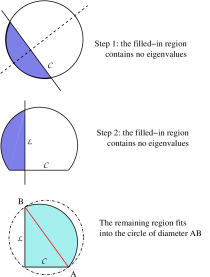
Figure 3: The 2-step strategy reduces the radius of the bounding box.

Thus, we are justified in assuming that $R=O(||A||)$; to sum up, we have the following corollary:

Corollary 3.7.

With probability at least $1-c\cdot\epsilon\cdot n\cdot f(n)\cdot\kappa(S)$, the number of iterations needed for progress at every step is at most $\log_{2}\frac{1}{c\epsilon f(n)}+\log_{2}\log_{2}\frac{1}{\epsilon}$.

3.3.1 Numerical experiments

Numerical experiments for Algorithm 5 are given in Figures 4 and 5. We chose four representative examples and present for each the distribution of the eigenvalues in the complex plane and the convergence plot of the backward error after a given number of iterations of implicit repeated squaring. This backward error is $\frac{\|E_{21}\|_{2}}{\|A\|_{2}}$ in the notation given in Algorithm 5, where the dimension of $E_{21}$ is chosen to minimize this quantity. In practice, a different test of convergence can be used for the implicit repeated squaring, but for demonstrative purposes, we computed the invariant subspace after each iteration of repeated squaring in order to show the convergence of the backward error of an entire step of divide-and-conquer.

The examples presented in Figure 4 are normal matrices generated by choosing random eigenvalues (where the real and imaginary parts are each chosen uniformly from $[-1.5,1.5]$) and applying a random orthogonal similarity transformation. The only difference is the matrix size. We point out that the convergence rate depends not on the size of the matrix but rather the distance between the splitting line (the imaginary axis) and the closest eigenvalue (as explained in the previous section). This geometric distance is the same as the distance to the nearest ill-posed problem because in this case, the condition number of the (orthogonal) diagonalizing similarity matrix is $1$. The distance between the imaginary axis and the nearest eigenvalue is $8.36\cdot 10^{-3}$ in Figure 4(a) ($n=100$) and $1.04\cdot 10^{-3}$ in Figure 4(b) ($n=1000$); note that convergence occurs at about the same iteration.

The examples presented in Figure 5 are meant to test the boundaries of convergence of Algorithm 5. While the eigenvalues in these examples are artificially chosen to be close to the splitting line (imaginary axis), our randomized higher level strategy for choosing splitting lines will ensure that such cases will be highly unlikely. Figure 5(a) presents an example where the eigenvalues are chosen with random imaginary part (between $-1.5$ and $1.5$) and real part set to $\pm 10^{-10}$ and the eigenvectors form a random orthogonal matrix. Because all the eigenvalues lie so close to the splitting line, convergence is much slower than in the examples with random eigenvalues. Note that because the imaginary axis does not intersect the $\epsilon$-pseudospectrum (where $\epsilon$ is machine precision), convergence is still achieved within $40$ iterations.

The example presented in Figure 5(b) is a 32-by-32 non-normal matrix which has half of its eigenvalues chosen randomly with negative real part and the other half set to $0.1$, forming a single Jordan block. In this example, the imaginary axis intersects the $\epsilon$-pseudospectrum and so Algorithm 5 does not converge. Note that the eigenvalue distribution in the plot on the left shows $16$ eigenvalues forming a circle of radius $0.1$ centered at $0.1$. The eigenvalue plots are the result of using standard algorithms which return $16$ distinct eigenvalues within the pseudospectral component containing $0.1$.

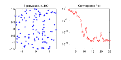
(a) $100\times 100$ matrix with random eigenvalues

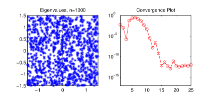
(b) $1000\times 1000$ matrix with random eigenvalues

Figure 4: Numerical experiments using normal matrices for Algorithm RNEP. On the left of each subfigure is a plot of the eigenvalues in the complex plane (as computed by standard algorithms) with the imaginary axis (where the split occurs) highlighted. In each case, the eigenvalues have real and imaginary parts chosen uniformly from $[-1.5,1.5]$. On the right is a convergence plot of the backward error as described in Section 3.3.1.

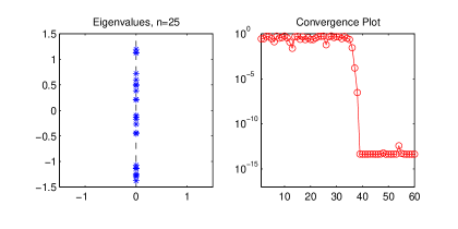
(a) $25\times 25$ matrix with eigenvalues whose real parts are $\pm 10^{-10}$

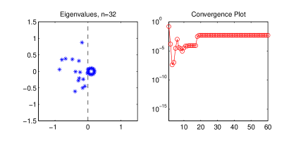
(b) $32\times 32$ matrix with half the eigenvalues forming Jordan block at $0.1$

Figure 5: Numerical experiments for Algorithm RNEP. On the left of each subfigure is a plot of the eigenvalues in the complex plane (as computed by standard algorithms) with the imaginary axis (where the split occurs) highlighted. Note in 5(a), all eigenvalues are at a distance of $10^{-10}$ from the imaginary axis. In 5(b), the imaginary axis intersects the $\epsilon$-pseudospectrum (where $\epsilon$ is machine precision). On the right is a convergence plot of the backward error as described in Section 3.3.1 for up to $60$ iterations.

3.4 High level strategy for divide-and-conquer, single symmetric matrix (or SVD) case

In this case, the eigenvalues are on the real line. After obtaining upper and lower bounds for the spectrum (e.g., Gershgorin intervals), we use vertical lines to split it. In order to try and split a large piece of the spectrum at a time, we will choose the lines to be close to the centers of the obtained intervals.

From Lemma 3 of [3] we can see that the basic splitting algorithm will converge if the splitting line does not intersect some $\hat{\epsilon}$-pseudospectrum of the matrix, which consists of a union of at most $n$ $2\hat{\epsilon}$-length intervals. Note that here we only consider symmetric perturbations to the matrix, and thus the pseudospectrum is a union of intervals.

To maximize the chances of a good split we will randomize the choice of splitting line, as follows: for an interval I, which can without loss of generality be taken as $[-R,R]$, we will choose a point $x$ uniformly between $[-R/2,R/2]$ and use the vertical line passing through $x$ for our split. See Figure 6 below.

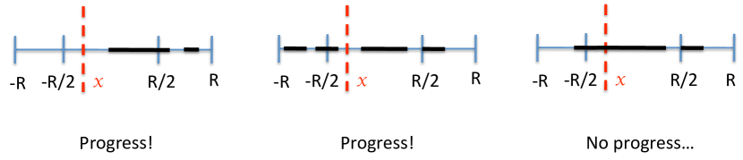
Figure 6: The possible outcomes of splitting the segment $[-R,R]$. The thick dark segments represent pseudospectral components (unions of overlapping smaller segments), while the dashed line represents the random choice of split.

As before, we measure progress in two ways: one is when a successful split occurs, i.e.,we separate some of the eigenvalues, and the second one is when no split occurs, but a large piece of the interval is determined not to contain any eigenvalues. Thus, progress can fail to occur in this context only if our choice of $x$ falls inside one (or more) of the small intervals representing the $\hat{\epsilon}$-pseudospectrum. The total length of these intervals is at most $2\hat{\epsilon}n$. Therefore, it is a simple calculation to show that the probability that a randomly chosen line in $[-R/2,R/2]$ will intersect the $\hat{\epsilon}$-pseudospectrum is larger than $1-2n\hat{\epsilon}/R$.

As before, the right choice for $\hat{\epsilon}$ must be proportional to $cf(n)||A||$, with $f(n)$ a polynomial of low degree; also as before, $R$ will be $O(||A||)$; putting these two together with Lemma 3.5, we get the following.

Corollary 3.8.

With probability at least $1-c\cdot\epsilon\cdot n\cdot f(n)$, the number of iterations is at most $\log_{2}\frac{1}{c\epsilon f(n)}+\log_{2}\log_{2}\frac{1}{\epsilon}$.

Finally, we note that a large cluster of eigenvalues actually helps convergence in the symmetric case, as the following lemma shows:

Lemma 3.9.

If $A=\left[\begin{array}[]{cc}A_{11}&A_{21}^{T}\\ A_{21}&A_{22}\end{array}\right]$ is hermitian, $\|A_{21}\|_{2}\leq(\lambda_{\max}(A)-\lambda_{\min}(A))/2$.

In other words if the eigenvalues are tightly clustered ($\lambda_{\max}(A)-\lambda_{\min}(A)$ is tiny) then the matrix must be nearly diagonal.

Proof.

Choose unit vectors $x$ and $y$ such that $y^{T}A_{21}x=\|A_{21}\|_{2}$, and let $z_{\pm}=2^{-1/2}\left[\begin{array}[]{c}x\\ \pm y\end{array}\right]$. Then $z_{\pm}^{T}Az_{\pm}=.5x^{T}A_{11}x+.5y^{T}A_{22}y\pm\|A_{21}\|_{2}$. So by the Courant-Fischer min-max theorem, $\lambda_{\max}(A)-\lambda_{\min}(A)\geq z_{+}^{T}Az_{+}-z_{-}^{T}Az_{-}=2\|A_{21}\|_{2}$. $\Box$

3.5 High level strategy for divide-and-conquer, general pencil case

Now we consider the case of a general square pencil defined by $(A,B)$, and how to reduce it to (block) upper triangular form by dividing-and-conquering the spectrum in an analogous way to the previous sections. Of course, in this generality the problem is not necessarily well-posed, for if the pencil is singular, i.e. the characteristic polynomial $\det(A-\lambda B)\equiv 0$ independent of $\lambda$, then every number in the extended complex plane can be considered an eigenvalue. Furthermore, arbitrarily small perturbations to $A$ and $B$ can make the pencil regular (nonsingular) with at least one (and sometimes all) eigenvalues located at any desired point(s) in the extended complex plane. (For example, suppose $A$ and $B$ are both strictly upper triangular, so we can change their diagonals to be arbitrarily tiny values with whatever ratios we like.)

The mathematically correct approach in this case is to compute the Kronecker Canonical Form (or rather the variant that only uses orthogonal transformations to maintain numerical stability [17, 18]), a problem that is beyond the scope of this paper.

The challenge of singular pencils is shared by any algorithm for the generalized eigenproblem. The conventional QZ iteration may converge, but tiny changes in the inputs (or in the level or direction of roundoff) will generally lead to utterly different answers. So “successful convergence” does not mean the answer can necessarily be used without further analysis. In contrast, our divide-and-conquer approach will likely simply fail to divide the spectrum when the pencil is close to a singular pencil. In the language of section 3.3, for a singular pencil the distance to any splitting line or circle is zero, and the $\epsilon$-pseudospectrum includes the entire complex plane for any $\epsilon>0$. When such repeated failures occur, the algorithm should simply stop and alert the user of the likelihood of near-singularity.

Fortunately, the set of singular pencils form an algebraic variety of high codimension [15], i.e. a set of measure zero, so it is unlikely that a randomly chosen pencil will be close to singular. Henceforth we assume that we are not near a singular pencil.

Even in the case of a regular pencil, we can still have eigenvalues that are arbitrarily large, or even equal to infinity, if $B$ is singular. So we cannot expect to find a single finite bounding circle holding all the eigenvalues, for example using Gershgorin disks [43], to which we could then apply the techniques of the last section, because many or all of the eigenvalues could lie outside any finite circle. Indeed, a Gershgorin disk in [43] has infinite radius as long as there is a common row of $A$ and $B$ that is not diagonally dominant.

In order to exploit the divide-and-conquer algorithm for the interior of circles developed in the last section, we proceed as follows: We begin by trying to divide the spectrum along the unit circle in the complex plane. If all the eigenvalues are inside, we proceed with circles of radius $2^{-2^{k}}$, i.e. radius $\frac{1}{2}$ and then repeatedly squaring, until we find a smallest such bounding circle, or (in a finite number of steps) run out of exponent bits in the floating point format (which means all the eigenvalues are in a circle of smallest possible representable radius, and we are done).

Conversely, if all the eigenvalues are outside, we proceed with circles of radius $2^{2^{k}}$, i.e. radius $2$ and repeatedly squaring, again until we either find a largest such bounding circle (all eigenvalues being outside), or we run out of exponent bits. At this point, we swap $A$ and $B$, taking the reciprocals of all the eigenvalues, so that they are inside a (small) circle, and proceed as in the last section. If the spectrum splits along a circle of radius $r$, with some inside (say those of $A_{11}-\lambda B_{11}$) and some outside (those of $A_{22}-\lambda B_{22}$), we instead compute eigenvalues of $B_{22}-\lambda A_{22}$ inside a circle of radius $\frac{1}{r}$.

3.6 Related work

As mentioned in the introduction, there have been many previous approaches to parallelizing eigenvalue/singular value computations, and here we compare and contrast the three closest such approaches to our own. These three algorithms are the PRISM project algorithm [6], the reduction of symmetric EIG to matrix multiplication by Yau and Lu [35], and the matrix sign function algorithm originally formulated in [26, 12, 36, 37, 38].

At the base of each of the approaches is the idea of computing, explicitly or implicitly, a matrix function $f(A)$ that maps the eigenvalues of the matrix (roughly) into $0$ and $1$, or $0$ and $\infty$.

3.6.1 The Yau-Lu algorithm

This algorithm essentially splits the spectrum in the symmetric case (as explained below), but instead of divide-and-conquer, which only aims at reducing the problem into two subproblems of comparable size, the Yau-Lu algorithm aims to break the problem into a large number of small subproblems, which can then be solved by classical methods.

The starting idea is put all the eigenvalues on the unit circle by computing $B=e^{iA}$; next, they use a Chebyshev polynomial $P_{N}(z)$ of high degree ($N\approx 8n$) to evaluate $u(\lambda)=P_{N}(e^{-i\lambda}B)v_{0}$ for $\lambda=\frac{ik\pi}{N}$ for $k=0,\ldots,N-1$. If $\lambda$ is close to an eigenvalue, $u(\lambda)$ will be close to the eigenvector ($P_{N}(z)$ has a peak at $z=1$, and is very close to $0$ everywhere except a small neighborhood of $z=1$ on the unit circle). They use the FFT to compute $u(\lambda)$ simultaneously for all $\lambda$, which makes things a lot faster ($O(n^{3}\log_{2}n)$ instead of $O(n^{4})$). This works only under the strong assumption that by scaling the eigenvalues so as to be between $0$ and $2\pi$, the gaps between them are all of order about $O(1/n)$.

Finally, they extract the most likely candidates for eigenvectors from among the $u(\lambda)$, split them into $p$ orthogonal clusters, add more vectors if necessary, construct an orthogonal basis $W$ whose elements span invariant subspaces of $A$, and thus obtain that $W^{T}AW$ decouples the spectrum, making it necessary and sufficient to solve $p$ small eigenvalue problems.

The authors make an attempt to perform an error analysis as well as a complexity analysis; neither completely addresses the case of tightly clustered eigenvalues. Clustering is a well-known challenge for attaining orthogonality with reasonable complexity, as highlighted in [19, 20].

By contrast, in the symmetric case, for highly clustered eigenvalues, our strategy would produce small bounding intervals and output them together with the number of eigenvalues to be found in them, as explained in the previous section.

3.6.2 Divide-and-conquer: the PRISM (symmetric) and sign function (both symmetric and non-symmetric) approaches

The algorithms [6, 26, 12, 38] can be described as follows. Given a matrix $A$:

1. Compute, explicitly or implicitly, a matrix function $f(A)$ that maps the eigenvalues of the matrix (roughly) into $0$ and $1$, or $0$ and $\infty$,

2. Do a rank-revealing decomposition (e.g. QR) to find the two spaces corresponding to the eigenvalues mapped to $1$ and $0$, or $\infty$ and $0$, respectively;

3. Block-upper-triangularize the matrix to split the problem into two or more smaller problems;

4. Recur on the diagonal blocks until all eigenvalues are found.

The strategy is thus to divide-and-conquer; issues of concern have to deal with the stability of the algorithm, the type and cost of the rank-revealing decomposition performed, the convergence of the first step, as well as the splitting strategy. We will try to address some of these issues below.

In the PRISM approach (for the symmetric eigenvalue, and hence by extension the SVD) [6], the authors choose Beta functions (polynomials which roughly approximate the step function from $[0,1]$ into $\{0,1\}$, with the step taking place at $1/2$) with or without acceleration techniques for their iteration. No stability analysis is performed, although there is reason to believe that some sort of forward stability could be achieved; the rank-revealing decomposition used is QR with pivoting. As such, there is also reason to believe that the approach is communication-avoiding, and that optimality can be reached by employing a lower-bound-achieving QR.

Since $f(A)$ is computed explicitly, one could potentially use a deterministic rank-revealing QR algorithm instead of our randomized one. There has been recent progress in developing such a QR algorithm that also minimizes communication [11].

The other approach is to use the sign function algorithm introduced by [40]; this works for both the symmetric and the non-symmetric cases, but requires taking inverses, which leads to a potential loss of stability. This can, however, be compensated for by ad-hoc means, e.g., by choosing a slightly different location to split the spectrum. In either case, some assumptions must be made in order to argue stability. A more in-depth discussion of algorithms using this method can be found in Section 3 of [3].

3.6.3 Our algorithm

Following in the footsteps of [3] and [14], we have used the basic algorithm of [26, 12, 36, 37, 38]. This algorithm was modified to be numerically stable and otherwise more practical (avoiding matrix exponentials) in [3]. It was then reduced to matrix multiplication and dense QR in [14] by introducing randomization in order to achieve the same arithmetic complexity as fast matrix multiplication (e.g. $O(n^{2.81})$ using Strassen’s matrix multiplication).

The algorithms we present here began as the algorithms in [14] and were modified to take advantage of the optimal communication-complexity $O(n^{3})$ algorithms for matrix multiplication and dense QR decomposition (the latter of which was given in [16]).

We also make here several contributions to the numerical analysis of the methods themselves. First, they depend on a rank-revealing generalized QR decomposition of the product of two matrices $A^{-1}B$, which is numerically stable and works with high probability. By contrast, this is done with pivoting in [3], and the pivot order depends only on $B$, whereas the correct choice obviously depends on $A$ as well. We know of no way to stably compute a rank-revealing generalized QR decomposition of expressions like $A^{-1}B$ without randomization. More generally, we show how to compute a randomized rank revealing QR decomposition of an arbitrary product of matrices (and/or inverses); some of the ideas were used in a deterministic context in G.W. Stewart’s paper [45], with application to graded matrices.

Second, we elaborate the divide-and-conquer strategy in considerably more detail than previous publications; the symmetric/SVD and non-symmetric cases differ significantly. The symmetric/SVD case returns a list of eigenvalues/eigenvectors (singular values/vectors) as usual; in the nonsymmetric case, the ultimate output may not be a matrix in Schur form, but rather block Schur form along with a bound (most simply a convex hull) on the $\epsilon$-pseudospectrum of each diagonal block, along with an indication that further refinement of the pseudospectrum is impossible without higher precision. For example, a single Jordan block would be represented (roughly) by a circle centered at the eigenvalue. A conventional algorithm would of course return $n$ eigenvalues evenly spaced along the circular border of the pseudospectrum, with no indication (without further computation) that this is the case. Both basic methods are oblivious to the genus of the pseudospectrum, as they will fail to point out “holes” like the one present in the third picture of Figure 1. In certain cases (like convex or almost convex pseudospectra) the information returned by divide-and-conquer may be more useful than the conventional method.

We emphasize that if a subproblem is small enough to solve by the standard algorithm using minimal communication, a list of its eigenvalues will be returned. So we will only be forced to return bounds on pseudospectra when the dimension of the subproblem is very large, e.g. does not fit in cache in the sequential case.

4 Communication Bounds for Computing the Schur Form

4.1 Lower bounds

We now provide two different approaches to proving communication lower bounds for computing the Schur decomposition. Although neither approach yields a completely satisfactory algorithm-independent proof of a lower bound, we discuss the merits and drawbacks as well as the obstacles associated with each approach.

The goal of the first approach is to show that computing the QR decomposition can be reduced to computing the Schur form of a matrix of nearly the same size. Such a reduction in principle provides a way to extend known lower bounds (communication or arithmetic) for QR decomposition to Schur decomposition, but has limitations described below.

We outline below a reduction of QR to a Schur decomposition followed by a triangular solve with multiple right hand sides (TRSM). There are two main obstacles to the success of this approach. First, the TRSM may have a nontrivial cost so that proving the cost of QR is at most the cost of computing Schur plus the cost of TRSM is not helpful. Second, all known proofs of lower bounds for QR apply to a restricted set of algorithms which satisfy certain assumptions, and thus the reduction is only applicable to Schur decomposition and TRSM algorithms which also satisfy those assumptions.

The first obstacle can be overcome with additional assumptions which are made explicit below. We do not see a way to overcome the second obstacle with the assumptions made in the current known lower bound proofs for QR decomposition, but future, more general proofs may be more amenable to the reduction.

We now give the reduction of QR decomposition to Schur decomposition and TRSM. Let $R$ be $m$-by-$m$ and upper triangular, $X$ be $n$-by-$m$ and dense, $A=\left[\begin{array}[]{c}R\\ X\end{array}\right]$ be $(m+n)$-by-$m$, and $B=\left[\begin{array}[]{cc}R&0^{m\times n}\\ X&0^{n\times n}\end{array}\right]$ be $(m+n)$-by-$(m+n)$. Let

$$A=\hat{Q}\cdot R_{A}=\left[\begin{array}[]{cc}Q_{11}&Q_{12}\\ Q_{21}&Q_{22}\end{array}\right]\cdot\left[\begin{array}[]{c}\hat{R}\\ 0^{n\times m}\end{array}\right]$$

where $\hat{R}$ and $Q_{11}$ are both $m$-by-$m$, and $Q_{22}$ is $n$-by-$n$. Note that $Q_{11}$ and $\hat{R}$ are both upper triangular. Then it is easy to confirm that the Schur decomposition of $B$ is given by

$$\hat{Q}^{T}\cdot B\cdot\hat{Q}=\left[\begin{array}[]{cc}\hat{R}\cdot Q_{11}&\hat{R}\cdot Q_{12}\\ 0^{n\times m}&0^{n\times n}\end{array}\right]\equiv\left[\begin{array}[]{cc}T_{11}&T_{12}\\ 0^{n\times m}&0^{n\times n}\end{array}\right]$$

Since $T_{11}$ is the upper triangular product of $\hat{R}$ and $Q_{11}$, we can easily solve for $\hat{R}=T_{11}\cdot Q_{11}^{-1}$. This leads to our reduction algorithm S2QR of the QR decomposition of $A$ to Schur decomposition of $B$ outline below. Note that here Schur stands for any black-box algorithm for computing the respective decomposition. In addition, TRSM stands for “triangular solve with multiple right-hand-sides”, which costs $O(m^{3})$ flops, and for which communication-avoiding implementations are known [4].

Algorithm 7 Function $[\hat{Q},\hat{R}]=$S2QR$([R;X])$, where $R$ is $n\times n$ upper triangular and $X$ is $m\times n$

1:  Form $B=\left[\begin{array}[]{cc}R&0\\ X&0\end{array}\right]$

2:  Compute $[\hat{Q},T]=$Schur$(B)$

3:  $Q_{11}=\hat{Q}(1:m,1:m)$; $T_{11}=T(1:m,1:m)$

4:  $\hat{R}=$TRSM$[Q_{11},T_{11}]$

5:  return  $[\hat{Q},\hat{R}]$

This lets us conclude that

$${\rm Cost}((m+n)\times(m+n)\;\mbox{{Schur}})\geq{\rm Cost}((m+n)\times(m)\>\mbox{{S2QR}})-{\rm Cost}((m)\times(m)\>\mbox{{TRSM}})$$

We assume now that we are using an “$O(n^{3})$ style” algorithm, which means that the cost of S2QR is $\Omega(m^{2}n)$, say at least $c_{1}m^{2}n$ for some constant $c_{1}$. Similarly, the cost of TRSM is $O(m^{3})$, say at most $c_{2}m^{3}$. We choose $m$ to be a suitable fraction of $n$, say $m=\min(.5c_{1}/c_{2},1)n$, so that

$${\rm Cost}((2n)\times(2n)\;{\rm\textbf{Schur}})\geq.5c_{1}m^{2}n=\Omega(n^{3})$$

as desired.

We note that this proof can provide several kinds of lower bounds:

• It provides a lower bound on arithmetic operations, by choosing $c_{1}$ to bound the number of arithmetic operations in S2QR from below [16], and $c_{2}=1/3$ to bound the number of arithmetic operations in TRSM from above [4].

• It can potentially provide a lower bound on the number of words moved (or the number of messages) in the sequential case, by taking $c_{1}$ and $c_{2}$ both suitably proportional to $1/M^{1/2}$ (or to $1/M^{3/2}$). We note that the communication lower bound proof in [4] does not immediately apply to this algorithm, because it assumed that the QR decomposition was computed (in the conventional backward-stable fashion) by repeated pre-multiplications of $A$ by orthogonal transformation, or by Gram-Schmidt, or by Cholesky-QR. However, this does not invalidate the above reduction.

• It can similarly provide a lower bound for all communication in the parallel case, assuming that the arithmetic work of both S2QR and TRSM are load balanced, by taking $c_{1}$ and $c_{2}$ both proportional to $1/P$.

The second approach to proving a communication lower bound for Schur decomposition is to apply the lower bound result for applying orthogonal transformations given by Theorem 4.2 in [4]. We must assume that the algorithm for computing Schur form performs $O(n^{3})$ flops which satisfy the assumptions of this result, to obtain the desired communication lower bound. This approach is a straightforward application of a previous result, but the main drawback is the loss of generality. Fortunately, this lower bound does apply to the spectral divide-and-conquer algorithm (by applying it just to the QR decompositions performed) as well as the first phase of the successive band reduction approach discussed in Section 6; this is all we need for a lower bound on the entire algorithm. But it does not necessarily apply to all future algorithms for Schur form.

The results of Theorem 4.2 in [4] require that a sequence of Householder transformations are applied to a matrix (perhaps in a blocked fashion) where the Householder vectors are computed to annihilate entries of a (possibly different) matrix such that forward progress is maintained, that is, no entry which has been previously annihilated is filled in by a later transformation. Therefore, this lower bound does not apply to “bulge-chasing,” the second phase of successive band reduction, where a banded matrix is reduced to tridiagonal form. But it does apply to the reduction of a full symmetric matrix to banded form via QR decomposition and two-sided updates, the first phase of the successive band reduction algorithms in Section 6.

Reducing a full matrix to banded form (of bandwidth $b$) requires $F=\frac{4}{3}n^{3}+bn^{2}-\frac{8}{3}b^{2}n+\frac{1}{3}b^{3}$ flops, so assuming forward progress, the number of words moved is at least $\Omega\left(\frac{F}{\sqrt{M}}\right)$, so for $b$ at most some fraction of $n$, we obtain a communication lower bound of $\Omega\left(\frac{n^{3}}{\sqrt{M}}\right)$.

4.2 Upper bounds: sequential case

In this section we analyze the complexity of the communication and computation of the algorithms described in Section 3 when performed on a sequential machine. We define $M$ to be the size of the fast memory, $\alpha$ and $\beta$ as the message latency and inverse bandwidth between fast and slow memory, and $\gamma$ as the flop rate for the machine. We assume the matrix is stored in contiguous blocks of optimal blocksize $b\times b$, where $b=\Theta(\sqrt{M})$. We will ignore lower order terms in this analysis, and we assume the original problem is too large to fit into fast memory (i.e., $an^{2}>M$ for $a=1,2$ or $4$).

4.2.1 Subroutines

The usual blocked matrix multiplication algorithm for multiplying square matrices of size $n\times n$ has a total cost of

$$C_{MM}(n)=\alpha\cdot O\left(\frac{n^{3}}{M^{3/2}}\right)+\beta\cdot O\left(\frac{n^{3}}{\sqrt{M}}\right)+\gamma\cdot O\left(n^{3}\right).$$

From [16], the total cost of computing the QR decomposition using the so-called Communication-Avoiding QR algorithm (CAQR) of an $m\times n$ matrix ($m\geq n$) is

$$C_{QR}(m,n)=\alpha\cdot O\left(\frac{mn^{2}}{M^{3/2}}\right)+\beta\cdot O\left(\frac{mn^{2}}{\sqrt{M}}\right)+\gamma\cdot O\left(mn^{2}\right)~{}.$$

This algorithm overwrites the upper half of the input matrix with the upper triangular factor $R$, but does not return the unitary factor $Q$ in matrix form (it is stored implicitly). To see that we may compute $Q$ explicitly with only a constant factor more communication and work, we could perform CAQR on the following block matrix:

$$\left[\begin{matrix}A&I\\ 0&0\end{matrix}\right]=\left[\begin{matrix}Q&0\\ 0&I\end{matrix}\right]\left[\begin{matrix}R&Q^{H}\\ 0&0\end{matrix}\right].$$

In this case, the block matrix is overwritten by an upper triangular matrix that contains $R$ and the conjugate-transpose of $Q$. For $A$ of size $n\times n$, this method incurs a cost of $C_{QR}(2n,2n)=O(C_{QR}(n,n))$. (This is not the most practical way to compute $Q$, but is sufficient for a $O(\cdot)$ analysis.) We note that an analogous algorithm (with identical cost) can be used to obtain RQ, QL, and LQ factorizations.

Computing the randomized rank-revealing QR decomposition (Algorithm 1) consists of generating a random matrix, performing two QR factorizations (with explicit unitary factors), and performing one matrix multiplication. Since the generation of a random matrix requires no more than $O(n^{2})$ computation or communication, the total cost of the RURV algorithm is

$$C_{RURV}(n) = 2\cdot C_{QR}(n,n)+C_{MM}(n)$$

$$= \alpha\cdot O\left(\frac{n^{3}}{M^{3/2}}\right)+\beta\cdot O\left(\frac{n^{3}}{\sqrt{M}}\right)+\gamma\cdot O\left(n^{3}\right).$$

We note that this algorithm returns the unitary factor $U$ and random orthogonal factor $V$ in explicit form. The analogous algorithm used to obtain the RULV decomposition has identical cost.

Performing implicit repeated squaring (Algorithm 3) consists of two matrix additions followed by iterating a QR decomposition of a $2n\times n$ matrix followed by two $n\times n$ matrix multiplications until convergence. Checking convergence requires computing norms of two matrices, constituting lower order terms of both computation and communication. Since the matrix additions also require lower order terms and assuming convergence after some constant $p$ iterations (depending on $\epsilon$, the accuracy desired, as per Corollaries 3.7 and 3.8), the total cost of the IRS algorithm is

$$C_{IRS}(n) = p\cdot\left(C_{QR}(2n,n)+2\cdot C_{MM}(n)\right)$$

$$= \alpha\cdot O\left(\frac{n^{3}}{M^{3/2}}\right)+\beta\cdot O\left(\frac{n^{3}}{\sqrt{M}}\right)+\gamma\cdot O\left(n^{3}\right).$$

Choosing the dimensions of the subblocks of a matrix in order to minimize the 1-norm of the lower left block (as in computing the $n-1$ possible values of $\|E_{21}\|_{1}/\|A\|_{1}+\|F_{21}\|_{1}/\|B\|_{1}$ in the last step of Algorithm 4) can be done with a blocked column-wise prefix sum followed by a blocked row-wise max reduction (the Frobenius and max-row-sum norms can be computed with similar two-phase reductions). This requires $O(n^{2})$ work, $O(n^{2})$ bandwidth, and $O\left(\frac{n^{2}}{M}\right)$ latency, as well as $O(n^{2})$ extra space. Thus, the communication costs are lower order terms when $an^{2}>M$.

4.2.2 Randomized Generalized Non-symmetric Eigenvalue Problem (RGNEP)

We consider the most general divide-and-conquer algorithm; the analysis of the other three algorithms differ only by constants. One step of RGNEP (Algorithm 4) consists of 2 evaluations of IRS, 2 evaluations of RURV, 2 evaluations of QR decomposition, and 6 matrix multiplications, as well as some lower order work. Thus, the cost of one step of RGNEP (not including the cost of subproblems) is given by

$$C_{RGNEP^{*}}(n) = 2\cdot C_{IRS}(n)+2\cdot C_{RURV}(n)+2\cdot C_{QR}(n,n)+6\cdot C_{MM}(n)$$

$$= \alpha\cdot O\left(\frac{n^{3}}{M^{3/2}}\right)+\beta\cdot O\left(\frac{n^{3}}{\sqrt{M}}\right)+\gamma\cdot O\left(n^{3}\right).$$

Here and throughout we denote by $C_{\text{ALG}^{*}}$ the cost of a single divide-and-conquer step in executing ALG.

Assuming we split the spectrum by some fraction $f$, one step of RGNEP creates two subproblems of size $fn$ and $(1-f)n$. If we continue to split by fractions in the range $[1-f_{0},f_{0}]$ at each step, for some threshold $\frac{1}{2}\leq f_{0}<1$, the total cost of the RGNEP algorithm is bounded by the recurrence

$$C(n)=\left\{\begin{array}[]{lr}C\left(f_{0}n\right)+C\left((1-f_{0})n\right)+C_{RGNEP^{*}}(n)&\text{if}\;\;2n^{2}>M\\ \alpha\cdot O(1)+\beta\cdot O(n^{2})+\gamma\cdot O\left(n^{3}\right)&\text{if}\;\;2n^{2}\leq M\end{array}\right.$$

where the base case arises when input matrices $A$ and $B$ fit into fast memory and the only communication is to read the inputs and write the outputs. This recurrence has solution

$$C(n)=\alpha\cdot O\left(\frac{n^{3}}{M^{3/2}}\right)+\beta\cdot O\left(\frac{n^{3}}{\sqrt{M}}\right)+\gamma\cdot O\left(n^{3}\right).$$

Note that while the cost of the entire problem is asymptotically the same as the cost of the first divide-and-conquer step, the constant factor for $C(n)$ is bounded above by $\frac{1}{3f_{0}(1-f_{0})}$ times the constant factor for $C_{RGNEP*}(n)$. That is, for constant $A$ defined such that $C_{RGNEP*}(n)\leq An^{3}$, we can verify that $C(n)\leq\frac{A}{3f_{0}(1-f_{0})}n^{3}$ satisfies the recurrence:

$$C(n) \leq C(f_{0}n)+C((1-f_{0})n)+C_{RGNEP*}(n)$$

$$\leq \frac{A}{3f_{0}(1-f_{0})}(f_{0}n)^{3}+\frac{A}{3f_{0}(1-f_{0})}((1-f_{0})n)^{3}+An^{3}$$

$$\leq \frac{(f_{0}^{3}+(1-f_{0})^{3})An^{3}+(3f_{0}(1-f_{0}))An^{3}}{3f_{0}(1-f_{0})}$$

$$\leq \frac{A}{3f_{0}(1-f_{0})}n^{3}.$$

4.3 Upper bounds: parallel case

In this section we analyze the complexity of the communication and computation of the algorithms described in Section 3 when performed on a parallel machine. We define $P$ to be the number of processors, $\alpha$ and $\beta$ as the message latency and inverse bandwidth between any pair of processors, and $\gamma$ as the flop rate for each processor. We assume the matrices are distributed in a 2D blocked layout with square blocksize $b=\frac{n}{\sqrt{P}}$. As before, we will ignore lower order terms in this analysis. After analysis of one step of the divide-and-conquer algorithms, we will describe how the subproblems can be solved independently.

4.3.1 Subroutines

The SUMMA matrix multiplication algorithm [25] for multiplying square matrices of size $n\times n$, with blocksize $b$, has a total cost of

$$C_{MM}(n,P)=\alpha\cdot O\left(\frac{n}{b}\log P\right)+\beta\cdot O\left(\frac{n^{2}}{\sqrt{P}}\log P\right)+\gamma\cdot O\left(\frac{n^{3}}{P}\right).$$

From [16] (equation (12) on page 62), the total cost of computing the QR decomposition using CAQR of an $n\times n$ matrix, with blocksize $b$, is

$$C_{QR}(n,n,P)=\alpha\cdot O\left(\frac{n}{b}\log P\right)+\beta\cdot O\left(\frac{n^{2}}{\sqrt{P}}\log P\right)+\gamma\cdot O\left(\frac{n^{3}}{P}+\frac{n^{2}b}{\sqrt{P}}\log P\right).$$

The cost of computing the QR decomposition of a tall skinny matrix of size $2n\times n$ is asymptotically the same.

As in the sequential case, RURV and IRS consist of a constant number of subroutine calls to the QR and matrix multiplication algorithms, and thus they have the following asymptotic complexity (here we assume a blocked layout, where $b=\frac{n}{\sqrt{P}}$):

$$C_{RURV}(n,P)=\alpha\cdot O\left(\sqrt{P}\log P\right)+\beta\cdot O\left(\frac{n^{2}}{\sqrt{P}}\log P\right)+\gamma\cdot O\left(\frac{n^{3}}{P}\log P\right),$$

and

$$C_{IRS}(n,P)=\alpha\cdot O\left(\sqrt{P}\log P\right)+\beta\cdot O\left(\frac{n^{2}}{\sqrt{P}}\log P\right)+\gamma\cdot O\left(\frac{n^{3}}{P}\log P\right).$$

Choosing the dimensions of the subblocks of a matrix in order to minimize the 1-norm of the lower left block (as in computing the $n-1$ possible values of $\|E_{21}\|_{1}/\|A\|_{1}+\|F_{21}\|_{1}/\|B\|_{1}$ in the last step of Algorithm 4) can be done with a parallel prefix sum along processor columns followed by a parallel prefix max reduction along processor rows (the Frobenius and max-row-sum norms can be computed with similar two-phase reductions). This requires $O\left(\log P\right)$ messages, $O\left(\frac{n}{\sqrt{P}}\log P\right)$ words, and $O\left(\frac{n^{2}}{P}\log P\right)$ arithmetic, which are all lower order terms, as well as $O\left(\frac{n^{2}}{P}\right)$ extra space.

4.3.2 Randomized Generalized Non-symmetric Eigenvalue Problem (RGNEP)

Again, we consider the most general divide-and-conquer algorithm; the analysis of the other three algorithms differ only by constants. One step of RGNEP (Algorithm 4) requires a constant number of the above subroutines, and thus the cost of one step of RGNEP (not including the cost of subproblems) is given by

$$C_{RGNEP^{*}}(n,P)=\alpha\cdot O\left(\sqrt{P}\log P\right)+\beta\cdot O\left(\frac{n^{2}}{\sqrt{P}}\log P\right)+\gamma\cdot O\left(\frac{n^{3}}{P}\log P\right).$$

Assuming we split the spectrum by some fraction $f$, one step of RGNEP creates two subproblems of sizes $fn$ and $(1-f)n$. Since the problems are independent, we can assign one subset of the processors to one subproblem and another subset of processors to the second subproblem. For simplicity of analysis, we will assign $f^{2}P$ processors to the subproblem of size $fn$ and $(1-f)^{2}P$ processors to the subproblem of size $(1-f)n$. This assignment wastes $2f(1-f)P$ processors ($\frac{1}{2}$ of the processors if we split evenly), but this will only affect our upper bound by a constant factor.

Because of the blocked layout, we assign processors to subproblems based on the data that resides in their local memories. Figure 7 shows this assignment of processors to subproblems where the split is shown as a dotted line. Because the processors colored light gray already own the submatrices associated with the larger subproblem, they can begin computation without any data movement. The processor owning the block of the matrix where the split occurs is assigned to the larger subproblem and passes the data associated with the smaller subproblem to an idle processor. This can be done in one message and is the only communication necessary to work on the subproblems independently.

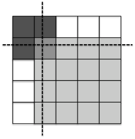
Figure 7: Assignment of processors to subproblems. The solid lines represent the blocked layout on 25 processors, the dotted line represents the subproblem split, and processors are color-coded for the subproblem assignment. One idle (white) processor is assigned to the smaller subproblem and receives the corresponding data from the processor owning the split.

If we continue to split by fractions in the range $[1-f_{0},f_{0}]$ at each step, for some threshold $\frac{1}{2}\leq f_{0}<1$, we can find an upper bound of the total cost along the critical path by accumulating the cost of only the larger subproblem at each step (the smaller problem is solved in parallel and incurs less cost). Although more processors are assigned to the larger subproblem, the approximate identity (ignoring logarithmic factors)

$$C_{RGNEP*}(fn,f^{2}P)\approx f\cdot C_{RGNEP*}(n,P)$$

implies that the divide-and-conquer step of the larger subproblem will require more time than the corresponding step for the smaller subproblem. If we assume that the larger subproblem is split by the largest fraction $f_{0}$ at each step, then the total cost of each smaller subproblem (including subsequent splits) will never exceed that of its corresponding larger subproblem. Thus, an upper bound on the total cost of the RGNEP algorithm is given by the recurrence

$$C(n,P)=\left\{\begin{array}[]{lr}C\left(f_{0}n,{f_{0}}^{2}P\right)+C_{RGNEP^{*}}(n,P)&\text{if}\;\;P>1\\ \gamma\cdot O\left(n^{3}\right)&\text{if}\;\;P=1\end{array}\right.$$

where the base case arises when one processor is assigned to a subproblem (requiring local computation but no communication). The solution to this linear recurrence is

$$C(n,P)=\alpha\cdot O\left(\frac{n}{b}\log P\right)+\beta\cdot O\left(\frac{n^{2}}{\sqrt{P}}\log P\right)+\gamma\cdot O\left(\frac{n^{3}}{P}+\frac{n^{2}b}{\sqrt{P}}\log P\right).$$

Here the constant factor for the upper bound on the total cost of the algorithm is $\frac{1-P^{-1/2}}{1-f_{0}}$ times larger than the constant factor for the cost of one step of divide-and-conquer. This constant arises from the summation $\sum_{i=0}^{d}{f_{0}}^{i}$ where $d=\log_{f_{0}}\frac{1}{\sqrt{P}}$ is the depth of the recurrence (we ignore the decrease in the size of the logarithmic factors).

Choosing the blocksize to be $b=\frac{n}{\sqrt{P}\log P}$, we obtain a total cost for the RGNEP algorithm of

$$C(n,P)=\alpha\cdot O\left(\sqrt{P}\log^{2}P\right)+\beta\cdot O\left(\frac{n^{2}}{\sqrt{P}}\log P\right)+\gamma\cdot O\left(\frac{n^{3}}{P}\right).$$

We will argue in the next section that this communication complexity is within polylogarithmic factors of optimal.

5 Computing Eigenvectors of a Triangular Matrix

After obtaining the Schur form of a nonsymmetric matrix $A=QTQ^{*}$, finding the eigenvectors of $A$ requires computing the eigenvectors of the triangular matrix $T$ and applying the unitary transformation $Q$. Assuming all the eigenvalues are distinct, we can solve the equation $TX=XD$ for the upper triangular eigenvector matrix $X$, where $D$ is a diagonal matrix whose entries are the diagonal of $T$. This implies that for $i<j$,

$$X_{ij}=\frac{\displaystyle T_{ij}X_{jj}+\sum_{k=i+1}^{j-1}T_{ik}X_{kj}}{T_{jj}-T_{ii}}$$ (15)

where $X_{jj}$ can be arbitrarily chosen for each $j$. We will follow the LAPACK naming scheme and refer to algorithms that compute the eigenvectors of triangular matrices as TREVC.

5.1 Lower bounds

Equation 15 matches the form specified in [4], where the $g_{ijk}$ functions are given by the multiplications $T_{ik}\cdot X_{kj}$. Thus we obtain a lower bound of the communication costs of any algorithm that computes these $O(n^{3})$ multiplies. That is, on a sequential machine with fast memory of size $M$, the bandwidth cost is $\Omega\left(\frac{n^{3}}{\sqrt{M}}\right)$ and the latency cost is $\Omega\left(\frac{n^{3}}{M^{3/2}}\right).$ On a parallel machine with $P$ processors and local memory bounded by $O\left(\frac{n^{2}}{P}\right)$, the bandwidth cost is $\Omega\left(\frac{n^{2}}{\sqrt{P}}\right)$ and the latency cost is $\Omega\left(\sqrt{P}\right).$

5.2 Upper bounds: sequential case

The communication lower bounds can be attained in the sequential case by a blocked iterative algorithm, presented in Algorithm 8. The problem of computing the eigenvectors of a triangular matrix, as well as the formulation of a blocked algorithm, appears as a special case of the computations presented in [29]; however, [29] does not try to pick a blocksize in order to minimize communication, nor does it analyze the communication complexity of the algorithm.

For simplicity we assume the blocksize $b$ divides $n$ evenly, and we use the notation $X[i,j]$ to refer to the $b\times b$ block of $X$ in the $i^{th}$ block row and $j^{th}$ block column. In this section and the next we consider the number of flops, words moved, and messages moved separately and use the notation $A_{ALG}$ to denote the arithmetic count, $B_{ALG}$ to denote to the bandwidth cost or word count, and $L_{ALG}$ to denote the latency cost or message count.

Algorithm 8 Blocked Iterative TREVC

0:  $T$ is upper triangular, $D$ is diagonal with diagonal entries of $T$; all matrices are blocked with blocksize $b\leq\sqrt{M/3}$ which divides $n$ evenly

1:  for $j=1$ to $n/b$ do

2:     solve $T[j,j]*X[j,j]=X[j,j]*D[j,j]$ for $X[j,j]$ {read $T[j,j]$, write $X[j,j]$}

3:     for $i=j-1$ down to $1$ do

4:        $S=0$

5:        for $k=i+1$ to $j$ do

6:           $S=S+T[i,k]*X[k,j]$ {read $T[i,k]$, read $X[k,j]$}

7:        end for{read $T[i,i]$, read $D[j,j]$, write $X[i,j]$}

8:     end for

9:  end for

9:  $X$ is upper triangular and $TX=XD$

Since each block has $O(b^{2})$ words, an upper bound on the total bandwidth cost of Algorithm 8 is given by the following summation and inequality:

$$B_{TREVC}(n) = \sum_{j=1}^{n/b}\left[O(b^{2})+\sum_{i=1}^{j-1}\left[\sum_{k=i+1}^{j}\left[O(b^{2})\right]+O(b^{2})\right]\right]$$

$$\leq \frac{n}{b}\left[O(b^{2})+\frac{n}{b}\left[\frac{n}{b}\left[O(b^{2})\right]+O(b^{2})\right]\right]$$

$$= O\left(\frac{n^{3}}{b}+n^{2}+nb\right).$$

If each block is stored contiguously, then each time a block is read or written, the algorithm incurs a cost of one message. Thus an upper bound on the total latency cost of Algorithm 8 is given by

$$L_{TREVC}(n) = \sum_{j=1}^{n/b}\left[O(1)+\sum_{i=1}^{j-1}\left[\sum_{k=i+1}^{j}\left[O(1)\right]+O(1)\right]\right]$$

$$= O\left(\frac{n^{3}}{b^{3}}+\frac{n^{2}}{b^{2}}+\frac{n}{b}\right).$$

Setting $b=\Theta(\sqrt{M})$, such that $b\leq\sqrt{M/3}$, we attain the lower bounds above (assuming $n^{2}>M$).

5.3 Upper Bounds: Parallel Case

There exists a parallel algorithm, presented in Algorithm 9, requiring $O(n^{2}/P)$ local memory that attains the communication lower bounds given above to within polylogarithmic factors. We assume a blocked distribution of the triangular matrix $T$ ($b=n/\sqrt{P}$) and the triangular matrix $X$ will be computed and distributed in the same layout. We also assume that $P$ is a perfect square. Each processor will store a block of $T$ and $X$, three temporary blocks $T^{\prime}$, $X^{\prime}$, and $S$, and one temporary vector $D$. That is, processor $(i,j)$ stores $T_{ij}$, $X_{ij}$, $T_{ij}^{\prime}$, $X_{ij}^{\prime}$, $S_{ij}$, and $D_{ij}$.

The algorithm iterates on block diagonals, starting with the main block diagonal and finishing with the top right block, and is “right-looking” (i.e. after the blocks along a diagonal are computed, information is pushed up and to the right to update the trailing matrix). Blocks of $T$ are passed right one processor column at a time, but blocks of $X$ must be broadcast to all processor rows at each step.

Algorithm 9 Parallel Algorithm PTREVC

0:  $T$ is upper triangular and distributed in blocked layout, $D$ is diagonal with diagonal entries of $T$ (no extra storage needed)

1:  for all processors $(i,j)$ such that $i\geq j$ do

2:     set $T_{ij}^{\prime}=T_{ij}$

3:     set $S_{ij}=0$

4:  end for

5:  for all processors $(j,j)$ do

6:     solve $T_{jj}X_{jj}=X_{jj}D_{jj}$ for $X_{jj}$ locally

7:     broadcast $X_{jj},D_{jj}$ up processor column, store in local $X^{\prime},D^{\prime}$

8:  end for

9:  for $k=1$ to $\sqrt{P}-1$ do

10:     for all processors $(i,j)$ such that $i-j\geq k-1$ do

11:        if $k\leq j<\sqrt{P}$ then

12:           send $T_{ij}^{\prime}\rightarrow T_{i,j+1}^{\prime}$ (to right)

13:        end if

14:        if $k<j\leq\sqrt{P}$ then

15:           receive $T_{i,j-1}^{\prime}\rightarrow T_{ij}^{\prime}$ (from left)

16:        end if

17:        if $i-j>k-1$ then

18:           update $S_{ij}=S_{ij}+T_{ij}^{\prime}X_{ij}^{\prime}$ locally

19:        end if

20:     end for

21:     for all processors $(i,j)$ such that $i-j=k$ do

22:        solve $T_{ij}^{\prime}X_{ij}+S_{ij}=X_{ij}D_{ij}^{\prime}$ for $X_{ij}$ locally

23:        broadcast $X_{ij}$ up processor column, store in local $X^{\prime}$

24:     end for

25:  end for

25:  $X$ is upper triangular and distributed in blocked layout, $TX=XD$

First we consider the arithmetic complexity. Arithmetic work occurs at lines 6, 18, and 22. All of the for loops in the algorithm, except for the one starting at line 9, can be executed in parallel, so the arithmetic cost of Algorithm 9 is given by

$$A_{TREVC}(n,P) = O\left(\left(\frac{n}{\sqrt{P}}\right)^{3}\right)+\sqrt{P}\left(O\left(\left(\frac{n}{\sqrt{P}}\right)^{3}\right)+O\left(\left(\frac{n}{\sqrt{P}}\right)^{3}\right)\right)$$

$$= O\left(\frac{n^{3}}{P}\right).$$

In order to compute the communication costs of the algorithm, we must make some assumptions on the topology of the network of the parallel machine. We will assume that the processors are arranged in a 2D square grid and that nearest neighbor connections exist (at least within processor rows) and each processor column has a binary tree of connections. In this way, adjacent processors in the same row can communicate at the cost of one message, and a processor can broadcast a message to all processors in its column at the cost of $O(\log P)$ messages.

Communication occurs at lines 7, 12, 15, and 23. Since every message is of size $O(n^{2}/P)$, the bandwidth cost of Algorithm 9 is given by

$$B_{TREVC}(n,P) = O\left(\frac{n^{2}}{P}\log P\right)+\sqrt{P}\left(O\left(\frac{n^{2}}{P}\right)+O\left(\frac{n^{2}}{P}\log P\right)\right)$$

$$= O\left(\frac{n^{2}}{\sqrt{P}}\log P\right)$$

and the latency cost is

$$L_{TREVC}(n,P) = O\left(\log P\right)+\sqrt{P}\left(O\left(1\right)+O\left(\log P\right)\right)$$

$$= O\left(\sqrt{P}\log P\right).$$

6 Successive Band Reduction

Here we discuss a different class of communication-minimizing algorithms, variants on the conventional reduction to tridiagonal form (for the symmetric eigenvalue problem) or bidiagonal form (for the SVD). These algorithms for the symmetric case were discussed at length in [7, 8], which in turn refer back to algorithms originating in [41, 42]. Our SVD algorithms are natural variations of these. These algorithms can minimize the number of words moved in an asymptotic sense on a sequential machine with two levels of memory hierarchy (say main memory and a cache of size $M$) when computing just the eigenvalues (respectively, singular values) or additionally all the eigenvectors (resp. all the left and/or right singular vectors) of a dense symmetric matrix (respectively, dense general matrix). Minimizing the latency cost, dealing with multiple levels of memory hierarchy, and minimizing both bandwidth and latency costs in the parallel case all remain open problems.

The algorithm for the symmetric case is as follows.

1. We reduce the original dense symmetric matrix $A$ to band symmetric form, $H=Q^{T}AQ$ where $Q$ is orthogonal and $H$ has bandwidth $b$. (Here we define $b$ to count the number of possibly nonzero diagonals above the main diagonal, so for example a tridiagonal matrix has $b=1$.) If only eigenvalues are desired, this step does the most arithmetic, $\frac{4}{3}n^{3}+O(n^{2})$ as well as $O(n^{3}/M^{1/2})$ slow memory references (choosing $b\approx\sqrt{M}$).

2. We reduce $H$ to symmetric tridiagonal form $T=U^{T}HU$ by successively zeroing out blocks of entries of $H$ and “bulge-chasing.” Pseudocode for this successive band reduction is given in Algorithm 10, and a scheme for choosing shapes and sizes of blocks to annihilate is discussed in detail below. This step does $O(n^{2}M^{1/2})$ floating point operations and, with the proper choice of block sizes, $O(n^{3}/M^{1/2})$ memory references. So while this step alone does not minimize communication, it is no worse than the previous step, which is all we need for the overall algorithm to attain $O(n^{3}/M^{1/2})$ memory references. If eigenvectors are desired, then there is a tradeoff between the number of flops and the number of memory references required (this tradeoff is made explicit in Table 1).

3. We find the eigenvalues of $T$ and–if desired–its eigenvectors, using the MRRR algorithm [20], which computes them all in $O(n^{2})$ flops, memory references, and space. Thus this step is much cheaper than the rest of the algorithm, and if only eigenvalues are desired, we are done.

4. If eigenvectors are desired, we must multiply the transformations from steps 1 and 2 times the eigenvectors from step 3, for an additional cost of $2n^{3}$ flops and $O(n^{3}/\sqrt{M})$ slow memory references.

Altogether, if only eigenvalues are desired, this algorithm does about as much arithmetic as the conventional algorithm, and attains the lower bound on the number of words moved for most matrix sizes, requiring $O(n^{3}/M^{1/2})$ memory references; in contrast, the conventional algorithm [1] moves $\Omega(n^{3})$ words in the reduction to tridiagonal form. However, if eigenvectors are also desired, the algorithm must do more floating point operations. For all matrix sizes, we can choose a band reduction scheme that will attain the asymptotic lower bound for the number of words moved and increase the number of flops by only a constant factor ($2\times$ or $2.6\times$, depending on the matrix size).

Algorithm 10 Successive band reduction of symmetric banded matrix

0:  $A\in\mathbb{R}^{n\times n}$ is symmetric with bandwidth $b=b_{1}$

1:  for $i=1$ to $s$ do

2:     {eliminate $d_{i}$ diagonals from band of remaining width $b_{i}$}

3:     for $j=1$ to $(n-b_{i})/c_{i}$ do

4:        {eliminate $c_{i}$ columns from bottom $d_{i}$ diagonals}

5:        zero out $d_{i}c_{i}$ entries of parallelogram by orthogonal transformation (e.g. parallelograms 1 and 6 in Figure 8)

6:        perform two-sided symmetric update, creating bulge (e.g. $Q_{1}$ creates bulge parallelogram 2 in Figure 8)

7:        for $k=1$ to $(n-jc_{i})/b_{i}$ do

8:           “chase the bulge” (zero out just the $d_{i}c_{i}$ entries of the parallelogram) (e.g. parallelograms 2 and 3 in Figure 8)

9:           perform two-sided symmetric update, creating bulge {(e.g. $Q_{3}$ creates bulge parallelogram 4 in Figure 8)}

10:        end for

11:     end for

12:     $b_{i+1}=b_{i}-d_{i}$

13:  end for

13:  $A$ is symmetric and tridiagonal

Table 1 compares the asymptotic costs for both arithmetic and communication of the conventional direct tridiagonalization with the two-step reduction approach outlined above. The analysis for Table 1 is given in Appendix A. There are several parameters associated with the two-step approach. We let $b$ denote the bandwidth achieved after the full-to-banded step. If we let $b=1$ we attain the direct tridiagonalization algorithm. If we let $b=\Theta(\sqrt{M})$, the full-to-banded step attains the communication lower bound. If eigenvectors are desired, then we form the orthogonal matrix $Q$ explicitly (at a cost of $\frac{4}{3}n^{3}$ flops) so that further transformations can be applied directly to $Q$ to construct $QU$, where $A=(QU)T(QU)^{T}$.

	# flops	# words moved
Direct Tridiagonalization
values	$\frac{4}{3}n^{3}$	$O\left(n^{3}\right)$
vectors	$2n^{3}$	$O\left(\frac{n^{3}}{\sqrt{M}}\right)$
Full-to-banded
values	$\frac{4}{3}n^{3}$	$O\left(\frac{n^{3}}{b}\right)$
vectors	$\frac{4}{3}n^{3}$	$O\left(\frac{n^{3}}{\sqrt{M}}\right)$
Banded-to-tridiagonal
values	$6bn^{2}$	$\displaystyle O\left(nb_{t}+\sum_{i=1}^{t-1}\left(1+\frac{d_{i}}{c_{i}}\right)n^{2}\right)$
vectors	$\displaystyle 2\sum_{i=1}^{s}\frac{d_{i}}{b_{i}}n^{3}$	$\displaystyle O\left(s\;\frac{n^{3}}{\sqrt{M}}\right)$

Table 1: Asymptotic computation and communication costs of reduction to tridiagonal form. Only the leading term is given in the flop count. The cost of the conventional algorithm is given in the first block row. The cost of the two-step approach is the sum of the bottom two block rows. If eigenvectors are desired, the cost of each step is the sum of the two quantities given. The parameter $t$ is defined such that $n(b_{t}+1)\leq M/4$, or, if no such $t$ exists, let $t=s+1$.

The set of parameters $s$, $b_{i}$, $c_{i}$, and $d_{i}$ (for $1\leq i\leq s$) characterizes the scheme for reducing the banded matrix $H$ to tridiagonal form via successive band reduction as described in [7, 8]. Over a sequence of $s$ steps, we successively reduce the bandwidth of the matrix by annihilating sets of diagonals ($d_{i}$ of them at the $i^{\text{th}}$ step). We let $b_{1}=b$ and

$$b_{i}=b-\sum_{j=1}^{i-1}d_{j}.$$

We assume that we reach tridiagonal form after $s$ steps, or that

$$\sum_{i=1}^{s}d_{i}=b-1.$$

Because we are applying two-sided similarity transformations, we can eliminate up to $b_{i}-d_{i}$ columns of the last $d_{i}$ subdiagonals at a time (otherwise the transformation from the right would fill in zeros created by the transformation from the left). We let $c_{i}$ denote the number of columns we eliminate at a time and introduce the constraint

$$c_{i}+d_{i}\leq b_{i}.$$

This process of annihilating a $d\times c$ parallelogram will introduce a trapezoidal bulge in the band of the matrix which we will chase off the end of the band. We note that we do not chase the entire trapezoidal bulge; we eliminate only the first $c_{i}$ columns (another $d\times c$ parallelogram) as that is sufficient for the next sweep not to fill in any more diagonals. These parameters and the bulge-chasing process are illustrated in Figure 8.

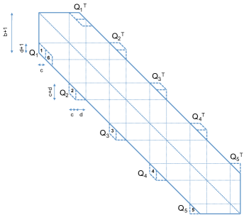
Figure 8: First pass of reducing a symmetric matrix from band to tridiagonal form. The numbers represent the order in which the parallelograms are eliminated, and $Q_{i}$ represents the orthogonal transformation which is applied to the rows and columns to eliminate the $i^{\text{th}}$ parallelogram.

We now discuss two different schemes (i.e. choices of $\{c_{i}\}$ and $\{d_{i}\}$) for reducing the banded matrix to tridiagonal form. Consider choosing $d_{1}=b-1$ and $c_{1}=1$, so that $s=1$, as in the parallel algorithm of [33]. Then the communication cost of the banded-to-tridiagonal reduction is $O(bn^{2})$. If we choose $b=\alpha_{1}\sqrt{M}$ for some constant $\alpha_{1}<1/2$, then four $b\times b$ blocks can fit into fast memory at a time, and by results in [16], the communication cost of reduction from full to banded form is $O\left(\frac{n^{3}}{\sqrt{M}}\right)$. The communication cost of the reduction from banded to tridiagonal (choosing $d_{1}=b-1$) is $O(n^{2}\sqrt{M})$, and so the total communication cost for reduction from full to tridiagonal form is $O\left(\frac{n^{3}}{\sqrt{M}}+n^{2}\sqrt{M}\right)$. This algorithm attains the lower bound if the first term dominates the second, requiring $n=\Omega(M)$. Thus, for sufficiently large matrices, this scheme attains the communication lower bound and does not increase the leading term of the flop count from the conventional method if only eigenvalues are desired.

If eigenvectors are desired, then the number of flops required to compute the orthogonal matrix $QU$ in the banded-to-tridiagonal step is $2n^{3}$ and the number of words moved in these updates is $O(n^{3}/\sqrt{M})$. If $T=V\Lambda V^{T}$ is the eigendecomposition of the tridiagonal matrix, then $A=(QUV)\Lambda(QUV)^{T}$ is the eigendecomposition of $A$. Thus, if the eigenvectors of $A$ are desired, we must also multiply the explicit orthogonal matrix $QU$ times the eigenvector matrix $V$, which costs an extra $2n^{3}$ flops and $O(n^{3}/\sqrt{M})$ words moved. Thus the communication lower bound is still attained, and the total flop count is increased to $\frac{20}{3}n^{3}$ as compared to $\frac{10}{3}n^{3}$ in the direct tridiagonalization.

Note that if $n<M$, the $n^{2}\sqrt{M}$ term dominates the communication cost and prevents the scheme above from attaining the lower bound. Consider values of $n$ that are larger than $\sqrt{M}$ (so the matrix does not fit into fast memory) but smaller than $M$ (so one or more diagonals do fit into fast memory). In this case, we reduce the banded matrix to tridiagonal in two steps ($s=2$). First, choose $d_{1}=b-\alpha_{2}\frac{M}{n}$ and $c_{1}=\alpha_{2}\frac{M}{n}$, where $\alpha_{2}<1/4$ is a constant chosen so that $\alpha_{2}\frac{M}{n}$ is an integer. This implies that $b_{2}=\alpha_{2}\frac{M}{n}$, so we choose $d_{2}=\alpha_{2}\frac{M}{n}-1$ and $c_{2}=1$, reducing to tridiagonal after two steps.

Suppose only eigenvalues are desired. Note that $nb_{2}=\alpha_{2}M$, so after the first pass, the band fits in fast memory. Note that we choose $\alpha_{2}<1/4$ so that the band itself fits in a quarter of fast memory, and another quarter of fast memory is available for bulges and other temporary storage. If eigenvectors are desired, then the other half of memory can be used in the computation of $QU$. Thus, the number of words moved in the reduction is $O(nb_{2}+(1+d_{1}/c_{1})n^{2})$. If we choose $b=\alpha_{1}\sqrt{M}$ for some constant $\alpha_{1}<1/2$, then $\frac{d_{1}}{c_{1}}=\Theta\left(\frac{n}{\sqrt{M}}\right)$, and the total communication cost for reduction from full to tridiagonal form is

$$O\left(\frac{n^{3}}{\sqrt{M}}+n^{2}+M\right)$$

and since $n^{2}>M$, the first term dominates and the scheme attains the lower bound. Again, the change in the number of flops in the reduction compared to the conventional algorithm is a lower order term.

If eigenvectors are desired, then the extra flops required to update the orthogonal matrix $Q$ to compute $QU$ is $2(\frac{d_{1}}{b_{1}}+\frac{d_{2}}{b_{2}})n^{3}$. Since $d_{i}<b_{i}$, this quantity is bounded by $4n^{3}$. Since we also have to multiply the updated orthogonal matrix $QU$ times the eigenvector matrix $V$ of the tridiagonal $T$ (for a cost of another $2n^{3}$ flops), this increases the total flop count to no more than $\frac{26}{3}n^{3}$. The extra communication cost of these updates is $O\left(\frac{n^{3}}{\sqrt{M}}\right)$ words, thus maintaining the asymptotic lower bound.

We may unify the two schemes for the two relative sizes of $n$ and $M$ as follows. Choose

$$b_{1} = \alpha_{1}\sqrt{M}$$

$$b_{2} = \max\left\{\alpha_{2}\frac{M}{n},1\right\}$$

$$d_{1} = b_{1}-b_{2}$$

$$c_{1} = b_{2}$$

where $\alpha_{1}<1/2,\alpha_{2}<1/4$ are constants, and, if necessary ($b_{2}>1$),

$$d_{2} = b_{2}-1$$

$$c_{2} = 1.$$

In this way we attain the communication lower bound whether or not eigenvectors are desired. If only eigenvalues are desired, then the two-step approach does $\frac{4}{3}n^{3}+O(n^{2})$ arithmetic which matches the cost of direct tridiagonalization. If eigenvectors are also desired, the number of flops required by the SBR approach is bounded by either $\frac{20}{3}n^{3}$ or $\frac{26}{3}n^{3}$ depending on the number of passes used to reduce the band to tridiagonal, as compared to the $\frac{10}{3}n^{3}$ flops required by the conventional algorithm.

$\sqrt{M}<n<M$	# flops	# words moved
Full-to-banded
$b=\alpha_{1}\sqrt{M}$
values	$\frac{4}{3}n^{3}$	$O\left(\frac{n^{3}}{\sqrt{M}}\right)$
vectors	$\frac{4}{3}n^{3}$	$O\left(\frac{n^{3}}{\sqrt{M}}\right)$
Banded-to-tridiagonal
$d_{1}=b-\alpha_{2}(M/n),\;c_{1}=\alpha_{2}(M/n)$
$d_{2}=b_{2}-1,\;c_{2}=1$
values	$6\alpha_{1}n^{2}\sqrt{M}$	$O\left(\frac{n^{3}}{\sqrt{M}}\right)$
vectors	$4n^{3}$	$O\left(\frac{n^{3}}{\sqrt{M}}\right)$
Recovering eigenvector matrix
vectors	$2n^{3}$	$O\left(\frac{n^{3}}{\sqrt{M}}\right)$
Total costs
values only	$\frac{4}{3}n^{3}$	$O\left(\frac{n^{3}}{\sqrt{M}}\right)$
values and vectors	$\frac{26}{3}n^{3}$	$O\left(\frac{n^{3}}{\sqrt{M}}\right)$

Table 2: Asymptotic computation and communication costs of reduction to tridiagonal form in the case of $\sqrt{M}<n<M$. The parameters $\alpha_{1}<1/2,\alpha_{2}<1/4$ are constants. Only the leading term is given in the flop count. The costs correspond to the specific choices of $b$, $d_{1}$, $c_{1}$, $d_{2}$, and $c_{2}$ listed in the first column.

$n>M$	# flops	# words moved
Full-to-banded
$b=\alpha_{1}\sqrt{M}$
values	$\frac{4}{3}n^{3}$	$O\left(\frac{n^{3}}{\sqrt{M}}\right)$
vectors	$\frac{4}{3}n^{3}$	$O\left(\frac{n^{3}}{\sqrt{M}}\right)$
Banded-to-tridiagonal
$d_{1}=b-1,\;c_{1}=1$
values	$6\alpha_{1}n^{2}\sqrt{M}$	$O\left(\frac{n^{3}}{\sqrt{M}}\right)$
vectors	$2n^{3}$	$O\left(\frac{n^{3}}{\sqrt{M}}\right)$
Recovering eigenvector matrix
vectors	$2n^{3}$	$O\left(\frac{n^{3}}{\sqrt{M}}\right)$
Total costs
values only	$\frac{4}{3}n^{3}$	$O\left(\frac{n^{3}}{\sqrt{M}}\right)$
values and vectors	$\frac{20}{3}n^{3}$	$O\left(\frac{n^{3}}{\sqrt{M}}\right)$

Table 3: Asymptotic computation and communication costs of reduction to tridiagonal form in the case of $n>M$. The constant $\alpha_{1}$ is chosen to be smaller than $1/2$. Only the leading term is given in the flop count. The costs correspond to the specific choices of $b$, $d_{1}$, and $c_{1}$ listed in the first column.

7 Conclusions

We have presented numerically stable sequential and parallel algorithms for computing eigenvalues and eigenvectors or the SVD, that also attain known lower bounds on communication, i.e. the number of words moved and the number of messages.

The first class of algorithms, which do randomized spectral divide-and-conquer, do several times as much arithmetic as the conventional algorithms, and are shown to work with high probability. Depending on the problem, they either return the generalized Schur form (for regular pencils), the Schur form (for single matrices), or the SVD. But in the case of nonsymmetric matrices or regular pencils whose $\epsilon$-pseudo-spectra include one or more large connected components in the complex plane containing very many eigenvalues, it is possible that the algorithm will only return convex enclosures of these connected components. In contrast, the conventional algorithm (Hessenberg QR iteration) would return eigenvalue approximations sampled from these components. Which kind of answer is more useful is application dependent. For symmetric matrices and the SVD, this issue does not arise, and with high probability the answer is always a list of eigenvalues.

A remaining open problem is to strengthen the probabilistic analysis of Theorem 2.1, which we believe underestimates the likelihood of convergence of our algorithm.

Given the Schur form of a nonsymmetric matrix or matrix pencil, we can also compute the eigenvectors in a communication-optimal fashion.

Our last class of algorithms uses a technique called successive band reduction (SBR), which applies only to the symmetric eigenvalue problem and SVD. SBR deterministically reduces a symmetric matrix to tridiagonal form (or a general matrix to bidiagonal form) after which a symmetric tridiagonal eigensolver (resp. bidiagonal SVD) running in $O(n^{2})$ time is used to complete the problem. With appropriate choices of parameters, sequential SBR minimizes the number of words moved between 2 levels of memory hierarchy; minimizing the number of words moved in the parallel case, or minimizing the number of messages in either the sequential or parallel cases are open problems. SBR on symmetric matrices only does double the arithmetic operations of the conventional, non-communication-avoiding algorithm when the matrix is large enough (or 2.6x the arithmetic when the matrix is too large to fit in fast memory, but small enough for one row or column to fit).

We close with several more open problems. First, we would like to extend our communication lower bounds so that they are not algorithm-specific, but algorithm-independent, i.e. apply for any algorithm for solving the eigenvalue problem or SVD. Second, we would like to do as little extra arithmetic as possible while still minimizing communication. Third, we would like to implement the algorithms discussed here and determine under which circumstances they are faster than conventional algorithms.

8 Acknowledgements

This research is supported by Microsoft (Award #024263) and Intel (Award #024894) funding and by matching funding by U.C. Discovery (Award #DIG07-10227). Additional support comes from Par Lab affiliates National Instruments, NEC, Nokia, NVIDIA, Samsung, and Sun Microsystems. James Demmel also acknowledges the support of DOE Grants DE-FC02-06ER25786, DE-SC0003959, and DE-SC0004938, and NSF Grant OCI-1032639. Ioana Dumitriu’s research is supported by NSF CAREER Award DMS-0847661. She would like to thank MSRI for their hospitality during the Fall 2010 quarter; this work was completed while she was a participant in the program Random Matrix Theory, Interacting Particle Systems and Integrable Systems.

Appendix A Analysis for Table 1

A.1 Direct Tridiagonalization

We now provide the analysis for the communication costs presented in Table 1. The flop counts for direct tridiagonalization are well-known, see [10], for example. Because direct tridiagonalization requires $n$ symmetric matrix-vector products (each requires moving $O(n^{2})$ data to access the matrix), the total number of words moved in reducing the symmetric matrix to tridiagonal is $O(n^{3})$. After this step, the orthogonal matrix whose similarity transformation tridiagonalizes $A$ is not stored explicitly, but as a set of Householder vectors. Applying these Householder vectors to the eigenvector matrix of the tridiagonal matrix to recover the eigenvectors of $A$ can be done in the usual blocked way and thus costs $2n^{3}$ and $O\left(\frac{n^{3}}{\sqrt{M}}\right)$ extra memory references if the blocksize is chosen to be $\Theta(\sqrt{M})$.

A.2 Counting Lemmas

To simplify the analysis for the rest of the table, we point out two useful facts. We also note that blocking Householder updates does introduce extra flops, but because the number of extra flops is a lower order term, we ignore them here and focus on BLAS-2 updates.

Lemma A.1.

The leading term of the number of flops required to apply a Householder transformation of a vector $u$ with $h$ nonzeros to $c$ columns (or rows if the applying from the right) of a matrix $A$ is $4hc$.

Proof.

Let $\tilde{A}$ be $m\times c$ (some subset of the columns of $A$). Applying the transformation associated with Householder vector $u$ is equivalent to overwriting the matrix $\tilde{A}$ with $\tilde{A}-\tau u(u^{T}\tilde{A})$. Since $u$ has $h$ nonzeros, the cost of computing $u^{T}\tilde{A}$ is $2hc$ which yields a dense row vector of length $c$. Computing $\tau u$ costs $h$ multiplies. Finally, $hc$ entries of $A$ must be updated with one multiplication and one subtraction each. Thus, the total cost of the update is $4hc+h$. $\Box$

Lemma A.2.

The cost of applying a Householder transformation of a vector with $h$ nonzeros from the left and right to a symmetric matrix is the same as applying the Householder transformation from the left to a nonsymmetric matrix of the same size.

Proof.

Let $A$ be $n\times n$ and symmetric, and let $u$ be a Householder vector with $h$ nonzeros. As pointed out in [21], the performing the following three computations overwrites the matrix $A$ with $(I-\tau uu^{T})A(I-\tau uu^{T})^{T}$:

$$y \leftarrow Au$$

$$v \leftarrow y-\frac{1}{2}(y^{T}u)u$$

$$A \leftarrow A-uv^{T}-vu^{T}$$

The first computation costs $2hn$ flops, and the second line costs $4h+1$. Since each of the matrices $uv^{T}$ and $vu^{T}$ have $hn$ nonzeros, each entry of $A$ which corresponds to a nonzero in one of the matrices must be updated with a multiplication and a subtraction. However, since $A$ is symmetric, we need to update only half of its entries, so the cost of the third line is $2hn$. Thus, the total cost (ignoring lower order terms) is $4hn$ which is the same as the cost of applying the Householder transformation from one side to an $n\times n$ nonsymmetric matrix. $\Box$

A.3 Reduction from Full to Banded

The second row of Table 1 corresponds to the first step of the SBR approach, reducing a full symmetric matrix to banded form by a sequence of QR factorizations on panels followed by two-sided updates. Algorithm 11 describes the reduction of a full symmetric matrix to banded form. Here TSQR refers to the Tall-Skinny QR decomposition described in [16], which returns $Q$ in a factored form whose details do not concern us here. The multiplication by $Q^{T}$ and $Q$ in the next two lines assumes $Q$ is in this factored form and exploits the symmetry of $A$. See [34] for the details of a multicore implementation of this algorithm. By Lemma A.2, the flop costs of the two-sided updates are the same as a one-sided update to a non-symmetric matrix. At the $k^{\text{th}}$ step of the reduction, the QR is performed on a panel of size $(n-kb)\times b$, yielding $(n-kb)b-\frac{1}{2}b^{2}$ Householder entries which are then applied to $n-kb+b$ rows and columns. Thus, by Lemma A.1, the arithmetic cost of the reduction is roughly

$$\sum_{k=1}^{n/b-2}2(n-kb)b^{2}-\frac{1}{3}b^{3}+4\left((n-kb)b-\frac{1}{2}b^{2}\right)(n-kb+b)=\frac{4}{3}n^{3}+O(bn^{2}).$$

By results for TSQR and applying $Q$ and $Q^{T}$ in Appendix B of [16], all of these flops may be organized in a blocked fashion to achieve a communication cost of $O\left(\frac{n^{3}}{b}\right)$ words, where $b<\sqrt{M}/2$. Note that $b<\sqrt{M}/2$ implies that $4b^{2}\leq M$, or four $b\times b$ blocks fit into fast memory at the same time.

Algorithm 11 Reduction of $A=A^{T}$ from dense to band form with bandwidth $b$

0:  $A\in\mathbb{R}^{n\times n}$ is symmetric, and assume that $b$ divides $n$ for simplicity

1:  for $i=1$ to $n-2b+1$ step $b$ do

2:     $[Q,R]=\text{TSQR}(A(i+b:n,i:i+b-1))$

3:     $A(i+b:n,:)=Q^{T}\cdot A(i+b:n,:)$

4:     $A(:,i+b:n)=A(:,i+b:n)\cdot Q$

5:  end for

5:  $A$ is symmetric and banded with bandwidth $b$

If eigenvectors are desired, the orthogonal matrix $Q$ that reduces the full matrix to banded form via similarity transformation is formed explicitly. In this way, the many small Householder transformations of the banded-to-tridiagonal step can be applied to $Q$ as they are computed and then discarded. The arithmetic cost of forming $Q$ explicitly is that of applying the Householder transformations to the identity matrix in reverse order as they were computed. Since the number of Householder entries used to reduce the second-to-last column panel is roughly $\frac{1}{2}b^{2}$ and the number of rows on which these transformations operate is $b$, the transformations need be applied only to the last $b$ columns of the identity matrix. The next set of transformations, computed to reduce the third-to-last column panel of $A$, operate on the last $2b$ rows. Thus, they need to be applied to only the last $2b$ columns of the identity matrix. Since the number of Householder entries used to reduce the $i^{\text{th}}$ column panel is roughly $(n-ib)b-\frac{1}{2}b^{2}$ and the number of columns to be updated is $(n-ib)$, by Lemma A.1, the total number of flops for constructing $Q$ explicitly is given by

$$\sum_{i=1}^{n/b-1}4\left((n-ib)b-\frac{1}{2}b^{2}\right)(n-ib)=\frac{4}{3}n^{3}+O(bn^{2}).$$

Again, as shown in [16], the application of these Householder entries can be organized so that the communication cost is $O\left(\frac{n^{3}}{b}\right)$ words where $b\leq\sqrt{M}/2$.

A.4 Reduction from Banded to Tridiagonal

Some analysis for the third row of Table 1 appears in [7] for the flop counts in the case $c_{i}=1$ for each $i$. We reproduce their results for general choices of $\{c_{i}\}$ and also provide analysis for the cost of the data movement. We will re-use the terminology from [7] and refer the reader to Figure 2(b) in that paper for a detailed illustration of one bulge-chase.

Bulge-chasing can be decomposed into four operations: “QR” of a $(d+c)\times c$ matrix, “Pre”-multiplication of an orthogonal matrix which updates $d+c$ rows, a two-sided “Sym”mmetric update of $(d+c)\times(d+c)$ submatrix, and “Post”-multiplication of the transpose of the orthogonal matrix which updates $d+c$ columns. We can count the arithmetic cost in terms of applying Householder vectors to sets of rows/columns (using Lemmas A.1 and A.2). Consider eliminating column $k$ of the parallelogram. In the QR step, the associated Householder transformation must be applied to the remaining $c-k$ columns. In the Pre step, the transformation is applied to $b-c$ columns. In the Sym step, the two-sided update is performed on a $(d+c)\times(d+c)$ submatrix. Finally, in the Post step, the transformation is applied from the right to $b-(c-k)$ rows. Since every Householder vector used to eliminate the parallelogram has $d$ nonzeros, the cost of eliminating each column of the parallelogram is $4d(2b+d)$, and the cost of eliminating the entire parallelogram ($c$ columns) is $8bcd+4cd^{2}$.

Bulge-chasing pushes the bulge $b$ columns down the band each time. Thus, the number of flops required to eliminate a set of $d$ diagonals is about

$$\sum_{j=1}^{n/c}\left(8bcd+4cd^{2}\right)\frac{n-jc}{b}=(4d+2\frac{d^{2}}{b})n^{2}.$$

Since $d<b$, this cost is bounded above by $6dn^{2}$. Taking $s$ steps to eliminate all the diagonals, we see that the total arithmetic cost of the banded-to-tridiagonal reduction (ignoring lower order terms) is

$$\sum_{k=i}^{s}6d_{i}n^{2}=6bn^{2}.$$

We now consider the data movement. First, suppose the band is small enough to fit into memory into one fourth of memory; that is, $n(b+1)<M/4$ (we pick the fraction $1/4$ so that the band fits in a quarter of the memory, the extra storage required for bulge chasing fits in a quarter of the memory, and the other half of memory can be reserved for the vector updating process discussed below). Then the communication cost of the reduction is simply reading in the band: $nb$ words. Suppose the band is too large to fit into memory. In this case, since we chase each bulge all the way down the band, we will obtain very little locality. Even though we eliminate a bulge as soon as it’s been created, we ignore the fact that some data (including the bulge itself) fits in memory and will be reused (it is a lower order term anyway). Consider the number of words accessed to chase one bulge: QR accesses $cd+\frac{1}{2}c^{2}$ words, Pre accesses $(b-c)(c+d)$ words, Sym accesses $\frac{1}{2}(c+d)^{2}$ words, and Post accesses $b(c+d)-\frac{1}{2}c^{2}$ words. The total number of words accessed for one bulge-chase is then $2b(c+d)+\frac{1}{2}(c+d)^{2}-c^{2}$. Using the same summation as before, the communication cost of chasing all the bulges from eliminating $d$ diagonals (ignoring lower order terms) is

$$\sum_{j=1}^{n/c}\left(2b(c+d)+\frac{1}{2}(c+d)^{2}-c^{2}\right)\frac{n-jc}{b}=\left(1+\frac{d}{c}-\frac{c}{2b}+\frac{(c+d)^{2}}{4bc}\right)n^{2}.$$

Since $c+d\leq b$, and by ignoring the negative term, we obtain a communication cost for eliminating $d$ diagonals of $O\left(\left(1+\frac{d}{c}\right)n^{2}\right)$.

In order to obtain the communication cost for the entire banded-to-tridiagonal step, we sum up the costs of all the reductions of $\{d_{i}\}$ diagonals until the band fits entirely in memory. That is, the number of words moved in the banded-to-tridiagonal step is

$$O\left(nb_{t}+\sum_{i=1}^{t-1}\left(1+\frac{d_{i}}{c_{i}}\right)n^{2}\right)$$

where $n(b_{t}+1)\leq M$. Note that if no such $t$ exists (in the case $2n>M$), the number of words is given by

$$O\left(\sum_{i=1}^{s}\left(1+\frac{d_{i}}{c_{i}}\right)n^{2}\right)$$

where $b_{s+1}=1$.

If eigenvectors are desired, each of the orthogonal transformations used to eliminate a parallelogram or chase a bulge must also be applied to the orthogonal matrix $Q$ which is formed explicitly in the full-to-banded step. Note that the transformations must be applied to $Q$ from the right (we are forming the matrix $QU$ such that $(QU)^{T}AQU=T$ is tridiagonal). However, these updates are one-sided and since many of the orthogonal transformations work on mutually disjoint sets of columns, we can reorder the updates to $Q$. The restrictions on this reordering are made explicit in [9], and we use the same reordering proposed in that paper. Note that to be able to reorder the updates on the eigenvector matrix $Q$, we must temporarily store a set of Householder entries which are computed in the band reduction process.

Suppose we save up all the Householder entries from eliminating $k$ parallelograms and chasing their associated bulges completely off the band. Since every Householder transformation consists of $cd$ Householder entries, saving up the transformations after eliminating $k$ parallelograms requires $O\left(kcd\frac{n}{b}\right)$ words of extra memory.

Following the notation of [9], we number the Householder transformations by the ordered pair $(i,j)$ where $i$ is the number of the initial parallelogram annihilated and $j$ is the number of the bulge chased by the transformation (so $1\leq i\leq k$ and $1\leq j\leq n/b$). For example, in Figure 8, $Q_{1}$ would we numbered $(1,1)$, $Q_{3}$ would be numbered $(1,3)$, and the orthogonal transformation annihilating parallelogram $6$ would be numbered $(2,1)$. We will group these Householder transformations not by their initial parallelogram number but by their bulge number (the second index in the ordered pair). As argued in [9], we can apply these updates in groups in reverse order, so that all $(i,4)$ transformations will be applied before any $(i,3)$ transformations. As long as the order of the updates within the groups is done in increasing order with respect to the initial parallelogram number (e.g. $(3,4)$ before $(4,4)$), we maintain correctness of the algorithm.

Consider the group of transformations with bulge number $j$. The transformation $(1,j)$ eliminates a parallelogram of size $d\times c$ and therefore updates $d+c$ columns of $Q$. Since the transformation $(2,j)$ eliminates the adjacent parallelogram, it updates an overlapping set of columns. The first (leftmost) $d$ columns are affected by $(1,j)$, but the last (rightmost) $c$ columns are disjoint. Since all of the parallelograms are adjacent, the total number of columns updated by the $k$ transformations with bulge number $j$ is $d+kc$.

We choose $k$ such that $kc=\Theta(\sqrt{M})$. Note that we may always choose $k$ in this way if we assume the initial bandwidth is chosen to be $b=O(\sqrt{M})$ since $c<b$ (this is a safe assumption because choosing a larger bandwidth does not reduce memory traffic in the full-to-banded step). This implies that since $d<b$, the extra memory required is $O(n\sqrt{M})$ words, each group of Householder transformations consists of $kcd=O(M)$ words, and that the number of columns affected by each group of Householder transformations is $O(\sqrt{M})$.

We now describe the updates to $Q$. We assume that all of the Householder entries for $k$ sweeps of the reduction process have been stored in slow memory and that $Q$ resides in slow memory. The updating process is given as Algorithm 12.

Algorithm 12 Updating eigenvector matrix $Q$ with Householder transformations from $k$ sweeps

0:  $Q\in\mathbb{R}^{n\times n}$ is orthogonal, transformations $U(i,j)$ have been computed for $1\leq i\leq k$ and $1\leq j\leq J$, and assume that $B$ divides $n$ for simplicity

1:  for $l=1$ to $n-B$ step $B$ do

2:     for $j=J$ down to $1$ do

3:        read $U(i,j)$ for $1\leq i\leq k$

4:        read columns of row panel $Q(i:i+B-1,:)$ (not already in fast memory) effected by $U(1:k,j)$

5:        for $i=1$ to $k$ do

6:           apply $U(i,j)$

7:        end for

8:     end for

9:  end for

9:  $Q$ is orthogonal

Let $J=O(n/b)$ be the largest bulge number. We update $Q$ one row panel at a time in reverse order by the bulge number $j$ and then in increasing order by sweep number $i$. Since the size of each group of transformations is $O(M)$, and the number of rows and columns of $Q$ accessed at each iteration are both $O(\sqrt{M})$, all of the necessary information resides in fast memory during the application of the $(i,j)$ transformations. The columns effected by transformations $(:,j)$ and $(:,j-1)$ may overlap, but since the rightmost column effected by block $j$ is to the right of the rightmost column effected by $j-1$ for each $j$, applying the blocks of transformations in this order ensures that the entries of each row panel of $Q$ are read from and written to slow memory no more than once. However, each Householder entry in a transformation is read once for each row panel updated. Thus, the number of words accessed to/from slow memory for the vector update after $k$ sweeps, under the choices $kc=\Theta(\sqrt{M})$ and $B=\Theta(\sqrt{M})$ is

$$\frac{n}{B}\left(kcd\frac{n}{b}+nB\right)=O(n^{2}).$$

The number of times this updating process must be done to eliminate $d$ diagonals is $\frac{n}{kc}$, and thus the total communication cost is $O\left(\frac{n^{3}}{\sqrt{M}}\right)$. If $s$ is the number of steps taken to reach tridiagonal form, the total extra number of words moved in order to update the vector matrix in the banded-to-tridiagonal step is

$$O\left(s\;\frac{n^{3}}{\sqrt{M}}\right).$$

After the matrices $QU$ and $T$ are computed, we use MRRR to find the eigenvalues and (if desired) the eigenvectors of $T$. In order to compute the eigenvectors of $A$ we must multiply the matrix $QU$ times the eigenvector matrix of $T$, and doing so costs $2n^{3}$ flops and $O(n^{3}/\sqrt{M})$ memory references.

Appendix B SVD via SBR

The situation for the SVD is analogous to the symmetric eigenvalue problem using symmetric band reduction:

1. We reduce the matrix $A$ to upper triangular band form $S=U^{T}AV$ with bandwidth $b\approx M^{1/2}$, and $U$ and $V$ are orthogonal.

2. We reduce $S$ to upper bidiagonal form $B=W^{T}SX$, where $W$ and $X$ are orthogonal. We again do this by successively zeroing out blocks of entries of $S$ of carefully chosen sizes.

3. We find the singular values of $B$, and its left and/or right singular vectors if desired. There are a number of algorithms that can compute just the singular values in $O(n^{2})$ flops and memory references, in which case we are done. But computing the singular vectors as well is more complicated: Extending MRRR from the symmetric tridiagonal eigenproblem to the bidiagonal SVD has been an open problem for many years, but an extension was recently announced [47], whose existence we assume here.

4. If singular vectors are desired, we must multiply the transformations from steps 1 and 2 times the singular vectors from step 3, for an additional cost of $O(n^{3})$ flops and $O(n^{3}/\sqrt{M})$ slow memory references.

The algorithm and analysis for the SVD are entirely analogous to the symmetric case. Algorithm 13 shows the first part of the reduction to bidiagonal form.

Algorithm 13 Reduction of $A$ from dense to upper triangular band form with bandwidth $b$

0:  $A\in\mathbb{R}^{n\times n}$, and assume that $b$ divides $n$ for simplicity

1:  for $i=1$ to $n-2b+1$ step $b$ do

2:     $[Q_{c},R_{c}]=TSQR(A(i:n,i:i+b-1))$

3:     $A(i:n,:)=Q_{c}^{T}\cdot A(i:n,:)$

4:     $[Q_{r},R_{r}]=TSQR((A(i:i+b-1,i+b:n))^{T})$

5:     $A(:,i+b:n)=A(:,i+b:n)\cdot Q_{r}$

6:  end for

6:  $A$ is banded upper triangular with bandwidth $b$

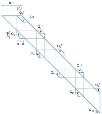
Figure 9: First pass of reducing a triangular matrix from banded to bidiagonal form

The first pass of the second part of the SVD algorithm, reducing the upper triangular band matrix to bidiagonal form, is shown in Figure 9. Table 4 provides the asymptotic computation and communication complexity of computing the SVD for the case when only singular values are desired and the case when both left and right singular vectors as well as the singular values are desired. The analysis for Table 4 is analogous to the symmetric case. Except in the case of the reduction from banded to bidiagonal form, the leading term in the flop count at each step doubles as compared to the symmetric eigenproblem.

	# flops	# words moved
Direct Bidiagonalization
values	$\frac{8}{3}n^{3}$	$O\left(n^{3}\right)$
vectors	$4n^{3}$	$O\left(\frac{n^{3}}{\sqrt{M}}\right)$
Full-to-banded
values	$\frac{8}{3}n^{3}$	$O\left(\frac{n^{3}}{b}\right)$
vectors	$\frac{8}{3}n^{3}$	$O\left(\frac{n^{3}}{\sqrt{M}}\right)$
Banded-to-tridiagonal
values	$8bn^{2}$	$\displaystyle O\left(nb_{t}+\sum_{i=1}^{t-1}\left(1+\frac{d_{i}}{c_{i}}\right)n^{2}\right)$
vectors	$\displaystyle 4\sum_{i=1}^{s}\frac{d_{i}}{b_{i}}n^{3}$	$\displaystyle O\left(s\;\frac{n^{3}}{\sqrt{M}}\right)$
Recovering singular vectors
vectors	$4n^{3}$	$\displaystyle O\left(\frac{n^{3}}{\sqrt{M}}\right)$

Table 4: Asymptotic computation and communication costs of computing the SVD of a square matrix. Only the leading term is given in the flop count. The cost of the conventional algorithm is given in the first block row. The cost of the two-step approach is the sum of the bottom three block rows. If both sets of singular vectors are desired, the cost of each step is the sum of the two quantities given. The parameter $t$ is defined such that $n(b_{t}+1)\leq M/4$, or, if no such $t$ exists, let $t=s+1$.

In order to attain the communication lower bound, we use the same scheme for choosing $b$, $\{c_{i}\}$, and $\{d_{i}\}$ as in the symmetric case. That is, for large matrices ($n>M$), we reduce the band to bidiagonal in one sweep, and for smaller matrices ($\sqrt{M}<n<M$), we use the first sweep to reduce the size of the band so that it fits in fast memory and the second sweep to reduce to bidiagonal form. As in the case of the symmetric eigenproblem, if only singular values are desired, the leading term in the flop count is the same as for the conventional, non-communication-avoiding algorithm. If both left and right singular vectors are desired, for large matrices, we increase the leading term in the flop count by a factor of $2$, and for smaller matrices, we increase the leading term in the flop count by a factor of $2.6$. The conventional approach costs $\frac{8}{3}n^{3}$ flops if only singular values are desired and $\frac{20}{3}n^{3}$ flops if all vectors and values are desired. Computing the SVD via SBR costs $\frac{8}{3}n^{3}$ flops if only singular values are required and either $\frac{40}{3}n^{3}$ or $\frac{52}{3}n^{3}$ flops if all vectors and values are desired.

References

- [1] E. Anderson, Z. Bai, C. Bischof, J. Demmel, J. Dongarra, J. Du Croz, A. Greenbaum, S. Hammarling, A. McKenney, S. Ostrouchov, and D. Sorensen. LAPACK Users’ Guide, Release 1.0. SIAM, Philadelphia, 1992. 235 pages.
- [2] L. Auslander and A. Tsao. On parallelizable eigensolvers. Advances in Applied Mathematics, 13:253–261, 1992.
- [3] Z. Bai, J. Demmel, and M. Gu. Inverse free parallel spectral divide and conquer algorithms for nonsymmetric eigenproblems. Num. Math., 76:279–308, 1997. UC Berkeley CS Division Report UCB//CSD-94-793, Feb 94.
- [4] G. Ballard, J. Demmel, O. Holtz, and O. Schwartz. Minimizing communication in linear algebra. SIAM Journal on Matrix Analysis and Applications, 2010. Submitted, available at http://arxiv.org/abs/0905.2485.
- [5] C. Bischof. Incremental condition estimation. SIAM, J. Mat. Anal. Appl., 11:312–322, 1990.
- [6] C. Bischof, S. Huss-Lederman, X. Sun, and A. Tsao. The PRISM project: Infrastructure and algorithms for parallel eigensolvers. In Proceedings of the Scalable Parallel Libraries Conference, Mississippi State, Mississippi. IEEE Computer Society, 1993.
- [7] C. Bischof, B. Lang, and X. Sun. A Framework for Successive Band Reduction. ACM Trans. Math. Software, 26(4):581–601, December 2000.
- [8] C. Bischof, B. Lang, and X. Sun. The SBR Toolbox: Software for Successive Band Reduction. ACM Trans. Math. Software, 26(4):602–616, December 2000.
- [9] C. Bischof, X. Sun, and B. Lang. Parallel tridiagonalization through two-step band reduction. In Scalable High-Performance Computing Conference. IEEE Computer Society Press, May 1994. (Also Prism Working Note #17 ftp.super.org:pub/prism).
- [10] L. S. Blackford, J. Choi, A. Cleary, J. Demmel, I. Dhillon, J. J. Dongarra, S. Hammarling, G. Henry, A. Petitet, K. Stanley, D. W. Walker, and R. C. Whaley. Scalapack: A portable linear algebra library for distributed memory computers - design issues and performance. In Proceedings of Supercomputing ’96. Sponsored by ACM SIGARCH and IEEE Computer Society, 1996. (ACM Order Number: 415962, IEEE Computer Society Press Order Number: RS00126. http://www.supercomp.org/sc96/proceedings/).
- [11] A. Branescu, J. Demmel, L. Grigori, M. Gu, and H. Xiang. Communication-avoiding rank-revealing QR decomposition. in preparation, 2010.
- [12] A. Ya. Bulgakov and S. K. Godunov. Circular dichotomy of the spectrum of a matrix. Siberian Math. J., 29(5):734–744, 1988.
- [13] Tony F. Chan and Per Christian Hansen. Some applications of the rank revealing QR factorization. SIAM J. Sci. Stat. Comput., 13(3):727–741, 1992.
- [14] J. Demmel, I. Dumitriu, and O. Holtz. Fast linear algebra is stable. Numerische Mathematik, 108(1):59–91, 2007.
- [15] J. Demmel and A. Edelman. The dimension of matrices (matrix pencils) with given Jordan (Kronecker) canonical forms. Lin. Alg. Appl., 230:61–87, 1995.
- [16] J. Demmel, L. Grigori, M. Hoemmen, and J. Langou. Communication-optimal parallel and sequential QR and LU factorizations. UC Berkeley Technical Report EECS-2008-89, Aug 1, 2008; Submitted to SIAM. J. Sci. Comp., 2008.
- [17] J. Demmel and Kågström. The generalized Schur decomposition of an arbitrary pencil : robust software with error bounds and applications. Part I – Theory and algorithms. ACM Trans. Math. Soft., 19(2):160–174, June 1993.
- [18] J. Demmel and Kågström. The generalized Schur decomposition of an arbitrary pencil : robust software with error bounds and applications. Part II – Software and applications. ACM Trans. Math. Soft., 19(2):175–201, June 1993.
- [19] I. S. Dhillon and B. N. Parlett. Orthogonal eigenvectors and relative gaps. SIAM J. on Matrix Analysis and Applications, 25(3):858–899, Mar 2004.
- [20] I. S. Dhillon, B. N. Parlett, and C. Voemel. The design and implementation of the mrrr algorithm. ACM Trans. Math.Soft., 32(4):533–560, Dec 2006.
- [21] Jack J. Dongarra, Sven Hammarling, and Danny C. Sorensen. Block reduction of matrices to condensed forms for eigenvalue computations. Technical Report 2, LAPACK Working Note, September 1987.
- [22] I. Dumitriu. Smallest eigenvalue distributions for -Jacobi ensembles. Electronic Journal of Probability, 2010. Submitted, available at http://arxiv.org/abs/1009.4677.
- [23] J. D. Frens and D. S. Wise. Qr factorization with morton-ordered quadtree matrices for memory re-use and parallelism. SIGPLAN Not., 38(10):144–154, 2003.
- [24] M. Frigo, C. E. Leiserson, H. Prokop, and S. Ramachandran. Cache-oblivious algorithms. In FOCS ’99: Proceedings of the 40th Annual Symposium on Foundations of Computer Science, page 285, Washington, DC, USA, 1999. IEEE Computer Society.
- [25] Robert A. Van De Geijn and Jerrell Watts. Summa: Scalable universal matrix multiplication algorithm. Concurrency: Practice and Experience, 9(4):255–274, 1997.
- [26] S. K. Godunov. Problem of the dichotomy of the spectrum of a matrix. Siberian Math. J., 27(5):649–660, 1986.
- [27] G. Golub and C. Van Loan. Matrix Computations. Johns Hopkins University Press, Baltimore, MD, 3rd edition, 1996.
- [28] M. Gu and S. C. Eisenstat. Efficient algorithms for computing a strong rank-revealing QR factorization. SIAM Journal on Scientific Computing, 17(4):848–869, 1996.
- [29] Greg Henry. The shifted hessenberg system solve computation. Technical report, Cornell Theory Center, 1995.
- [30] J. W. Hong and H. T. Kung. I/O complexity: The red-blue pebble game. In STOC ’81: Proceedings of the thirteenth annual ACM symposium on Theory of computing, pages 326–333, New York, NY, USA, 1981. ACM.
- [31] J. Howland. The sign matrix and the separation of matrix eigenvalues. Lin. Alg. Appl., 49:221–232, 1983.
- [32] D. Irony, S. Toledo, and A. Tiskin. Communication lower bounds for distributed-memory matrix multiplication. J. Parallel Distrib. Comput., 64(9):1017–1026, 2004.
- [33] B. Lang. A parallel algorithm for reducing symmetric banded matrices to tridiagonal form. SIAM J. Sci. Comput., 14(6), November 1993.
- [34] H. Ltaief, J. Kurzak, J. Dongarra, and R. Badia. Scheduling two-sided transformations using tile algorithms on multicore architectures. Journal of Scientific Computing, Vol. 18, No. 1:33–50, 2010.
- [35] Y. Lu and S. Yau. Eigenvalues of the Laplacian through boundary integral equations. SIAM J. Mat. Anal. Appl., 12(3):597–609, July 1991.
- [36] A. N. Malyshev. Computing invariant subspaces of a regular linear pencil of matrices. Siberian Math. J., 30(4):559–567, 1989.
- [37] A. N. Malyshev. Guaranteed accuracy in spectral problems of linear algebra, I,II. Siberian Adv. in Math., 2(1,2):144–197,153–204, 1992.
- [38] A. N. Malyshev. Parallel algorithm for solving some spectral problems of linear algebra. Lin. Alg. Appl., 188,189:489–520, 1993.
- [39] L. Reichel and L. N. Trefethen. Eigenvalues and pseudo-eigenvalues of Toeplitz matrices. Lin. Alg. Appl., 162–164:153–185, 1992.
- [40] J. Roberts. Linear model reduction and solution of the algebraic Riccati equation. Inter. J. Control, 32:677–687, 1980.
- [41] H. Rutishauser. On Jacobi rotation patterns. In N. Metropolis, A. Taub, J. Todd, and C. Tompkins, editors, Proceedings of Symposia in Applied Mathematics, Vol. XV: Experimental Arithmetic, High Speed Computing and Mathematics. American Mathematical Society, 1963.
- [42] H. Schwarz. Tridiagonalization of a symetric band matrix. Numerische Mathematik, 12:231–241, 1968.
- [43] G. W. Stewart. Gershgorin theory for the generalized eigenproblem . Math. Comp., 29(130):600–606, 1975.
- [44] G. W. Stewart. Rank degeneracy. SIAM J. Sci. Stat. Comput., 5:403–413, 1984.
- [45] G. W. Stewart. On graded QR decompositions of products of matrices. Electronic Transactions on Numerical Analysis, 3:39–49, 1995.
- [46] L. N. Trefethen and M. Embree. Spectra and Pseudospectra: The Behavior of Nonnormal Matrices and Operators. Princeton University Press, Princeton, NJ, 2005.
- [47] P. Willems. On MRRR-type algorithms for the tridiagonal symmetric eigenproblem and the bidiagonal SVD. PhD thesis, University of Wuppertal, 2009.