2D and 3D reconstructions in acousto-electric tomography

Abstract

We propose and test stable algorithms for the reconstruction of the internal conductivity of a biological object using acousto-electric measurements. Namely, the conventional impedance tomography scheme is supplemented by scanning the object with acoustic waves that slightly perturb the conductivity and cause the change in the electric potential measured on the boundary of the object. These perturbations of the potential are then used as the data for the reconstruction of the conductivity. The present method does not rely on “perfectly focused” acoustic beams. Instead, more realistic propagating spherical fronts are utilized, and then the measurements that would correspond to perfect focusing are synthesized. In other words, we use synthetic focusing. Numerical experiments with simulated data show that our techniques produce high quality images, both in $2D$ and $3D$, and that they remain accurate in the presence of high-level noise in the data. Local uniqueness and stability for the problem also hold.

Introduction

Electrical Impedance Tomography (EIT) is a harmless and inexpensive imaging modality, with important clinical and industrial applications. It aims to reconstruct the internal conductivity of a body using boundary electric measurements (see, e.g., [6, 4, 8, 9]). It is well known that, regretfully, it suffers from inherent low resolution and instability. To bypass this difficulty, various versions of a new hybrid technique, sometimes called Acousto-Electric Tomography (AET), have been introduced recently [3, 16, 25, 7]. (See also [12] for a different way to recover the conductivity using combination of ultrasound and EIT). AET utilizes the electro-acoustic effect, i.e. occurrence of small changes in tissue conductivity as the result of applied acoustic pressure [20, 21]. Although the effect is small, it was shown in [25] that it provides a signal that can be used for imaging the conductivity. It has been understood [3, 16, 7] that if one could apply concentrated pressure at a given point inside the body and then measure the resulting change in impedance measurements, the knowledge of the perturbation point would have a stabilizing effect on the reconstruction in otherwise highly unstable EIT. It has been proposed to use a tightly focused ultrasound beam as a source of such point-like acoustic pressure [3]. However, since perfect focusing of acoustic waves is hard to achieve in practice (see, e.g., [14]), an alternative synthetic focusing approach was developed in [16]. Namely, the medium is perturbed by a series of more realistic propagating spherical acoustic fronts with centers lying outside of the object (other options, e.g. plane waves or monochromatic spherical waves could also be used [16]). The resulting changes in the values of electric potential on the boundary of the object are recorded. Then the data that would have been collected, if perfect focusing were possible, are synthesized mathematically. Such synthesis happens to be equivalent to the well established inversion in the so called thermoacoustic tomography (see, e.g., the surveys [23, 24, 15]). Of course, for accurate synthesis the acoustic properties of the medium should be known. In breast imaging, for example, the speed of sound in the tissue can be well approximated by a constant, and application of AET in this area looks very promising. In the inhomogeneous medium synthetic focusing is possible if its acoustic parameters are reconstructed beforehand (for example, using methods of ultrasound tomography). The results of first numerical experiments presented in [16] confirm the feasibility of the synthetic focusing.

In this article, we describe a stable and efficient local algorithm for the AET problem. From the formulas we present one can easily infer the local uniqueness and stability of the reconstruction. However, after this work was done, the authors have learned of the paper [7], some results of which (Propositions 2.1, 2.2) imply uniqueness and Lipschitz stability in the similar setting (see also [5] for the presentation of such a local result). We thus address these issues only briefly here.

The presented algorithm involves two steps. First, it synthesizes the data corresponding to perfectly focused ultrasound perturbations from the data obtained using more realistic spherical waves. Here the known smallness of the acousto-electric effect [20, 21, 25] is crucial, since it permits linearization with respect to the acoustic perturbation and thus makes synthetic focusing possible. Second, the algorithm reconstructs the conductivity from the data corresponding to perfectly focused perturbations. This second step, from measured data to the conductivity, is non-linear. We develop a linearized algorithm, assuming that the conductivity is close to a known one. The numerical examples that we provide show that this approach works surprisingly well even when the initial guess is very distinct from the correct conductivity. One can apply iterations for further improvements.

To the best of the authors’ knowledge, the first step of our method (synthetic focusing) has not been discussed previously in works on AET, except for a brief description in our papers [16, 18]. On the other hand, three different approaches to reconstruction using perfectly focused beam (the second step of our algorithm) have been recently proposed [3, 16, 7, 18]. Let us thus indicate the differences with these recent works.

In [3], two boundary current profiles were used and the problem of reconstructing the conductivity was reduced to a numerical solution of a (non-linear) PDE involving the $0$-Laplacian. In [16, 18], by a rather crude approximation, we reduced the reconstruction problem to solving a transport equation (a single current was used). Unfortunately, in the case of noisy measurements the errors tend to propagate along characteristics, producing unpleasant artifacts in the images, which can be reduced by iterations. There is also a version of this procedure that involves an elliptic equation and thus works better. In [7], two current profiles are used in $2D$ (three profiles in $3D$), the problem is reduced to a minimization problem, which is then solved numerically. In the present paper we also use two currents in $2D$ (two or three in $3D$) and, on the second step, we utilize the same data as in [7]. Unlike [7], in our work the reconstruction problem is solved, under the assumption that the conductivity is close to some initial guess, by a simple algorithm, which even on the first step produces good images, improved further by iterations. The algorithm essentially boils down to solving a Poisson equation. Numerical experiments show high quality reconstructions, quite accurate even in the presence of very significant noise. Reconstructions remain accurate when the true conductivity differs significantly from the initial guess.

The rest of the paper is organized as follows: Section 1 contains the formulation of the problem. It also addresses the focusing issue. The next Section 2 describes the reconstruction algorithm, stability of which is discussed in Section 3. Numerical implementation and results of reconstruction from simulated data in $2D$ are described in Section 4. Sections 5 and 6 are addressing the $3D$ case. Section 7 is devoted to final remarks and conclusions.

1 Formulation of the problem

Let $\sigma(x)$ be the conductivity of the medium within a bounded region $\Omega$. Then the propagation of the electrical currents through $\Omega$ is governed by the divergence equation

$$\nabla\cdot\sigma(x)\nabla u(x)=0,x\in\Omega.$$ (1)

or, equivalently

$$\Delta u(x)+\nabla u(x)\cdot\nabla\ln\sigma(x)=0,$$ (2)

where $u(x)$ is the electric potential. Let us assume that $\sigma-1$ is compactly supported within region $\Omega,$ and that $\sigma(x)=1$ in the neighborhood of the boundary $\partial\Omega.$ We also assume that the currents $J=\sigma\frac{\partial}{\partial n}u(x)$ through the boundary are fixed and the values of potential $u$ are measured on the boundary $\partial\Omega$.

The acoustic wave propagating through the object slightly perturbs the conductivity $\sigma(x)$. Following the observations made in [20, 21], we assume that the perturbation is proportional to the local value of the conductivity; thus, the perturbed conductivity $\sigma^{new}(x)$ equals to $\sigma(x)\exp(\eta(x))$, where the perturbation exponent $\eta(x)$ is such that $|\eta(x)|\ll 1$ and is compactly supported. Let $u^{new}(x)=u(x)+w_{\eta}(x)$ be the potential corresponding to the perturbed conductivity $\sigma^{new}(x)$ and $w_{\eta}(x)$ be the perturbation thereof. By substituting these perturbed values into (2) one obtains

$$\Delta\left[u(x)+w_{\eta}(x)\right]+\nabla\left[u(x)+w_{\eta}(x)\right]\cdot\nabla\left[\ln\sigma(x)+\eta(x)\right]=0.$$ (3)

Further, by neglecting second order terms (in $\eta$) and by subtracting (2) from (3) we arrive at the the following equation:

$$\Delta w_{\eta}(x)+\nabla w_{\eta}(x)\cdot\nabla\ln\sigma(x)=-\nabla u(x)\cdot\nabla\eta(x).$$ (4)

Finally, by multiplying (4) by $\sigma(x)$ we find that $w_{\eta}(x)$ satisfies equation

$$\nabla\cdot\sigma(x)\nabla w_{\eta}(x)=-\sigma(x)\nabla u(x)\cdot\nabla\eta(x)$$ (5)

subject to the homogeneous Neumann boundary conditions. Since the values of $u(x)$ and $u^{new}(x)$ are measured on the boundary, the Dirichlet data for $w_{\eta}(x)$ are known. It will be sufficient for our purposes to measure a certain functional of the boundary values of $w_{\eta}(x)$. Let us fix a function $I(z)$ defined on $\partial\Omega$, and define the corresponding measurement functional $M_{I}(\eta)$ as follows:

$$M_{I,J}(\eta):=\int\limits_{\partial\Omega}w_{\eta}(z)I(z)dz.$$ (6)

Here the subscript $J$ on the left reminds about the dependence of $w$ on the current $J$. Function $I(z)$ does not have to be a function in the classical sense; it may also be chosen to be a distribution, for example a sum of delta-functions. In the latter case it would model measurements obtained by a set of point-like electrodes. Since the data corresponding to all electrodes then would be added together, the noise sensitivity of such a scheme is quite low, and our numerical experiments (not presented here) confirm that.

Our goal is to reconstruct $\sigma(x)$ from measurements of $M_{I,J}(\eta)$ corresponding to a sufficiently rich set of perturbations $\eta(x)$ in (5).

The simplest case is when one can achieve perfect focusing, and thus $\eta_{y}(x)\approx C\delta(x-y)$, where the point $y$ scans through $\Omega$. Then the reconstruction needs to be done from the values

$$M_{I,J,\delta}(y):=\int\limits_{\partial\Omega}w_{\eta_{y},J}(z)I(z)dz.$$

However, this assumption of perfect focusing is unrealistic [14]. More realistic are, for instance, mono-chromatic planar or spherical waves, or spreading spherical fronts. We assume here that ideal point-like transducers are excited by an infinitesimally short electrical pulse. If we assume (without loss of generality) that the speed of sound equals 1, the acoustic pressure $W_{t,z}(x)$ generated by a transducer placed at point $z$ (outside $\Omega$) solves the following initial value problem for the wave equation:

$$\begin{cases}\Delta_{x}W_{t,z}(x)=\frac{\partial^{2}}{\partial t^{2}}W_{t,z}(x),\quad x\in\mathbb{R}^{3},\quad t\in[0,\infty)\\ W_{0,z}(x)=\delta(|x-z|),\\ \frac{\partial}{\partial t}W_{0,z}(x)=0.\end{cases}.$$

Solution of this problem is well-known [22]:

$$W_{t,z}(x)=\frac{\partial}{\partial t}\left(\frac{\delta(t-|x-z|)}{4\pi t}\right);$$ (7)

it has the form of the propagating spherical front with the radius $t$ centered at $z$. (The time derivative of the $\delta$-function in (7) results naturally from the $\delta$-excitation of the transducer; the spherical waves we used in [16] can be obtained by anti-differentiation of the signal corresponding to (7).)

The perturbation $\eta_{t,z}(x)$ of the conductivity caused by the propagating front $W_{t,z}(x)$ equals $\eta_{0}W_{t,z}(x)$, where $\eta_{0}$ is some small fixed proportionality constant (reflecting the smallness of the acousto-electric effect). The corresponding measurements then are (after factoring out $\eta_{0}$):

$$M_{I,J}(t,z):=\int\limits_{\partial\Omega}w_{W_{t,z},J}(z)I(z)dz.$$ (8)

Due to the linear dependence of the measurements on the acoustic perturbation $\eta$, one can try to do a “basis change” type of calculation, which would produce the “focused” data $M_{I,J,\delta}(y)$ from the more realistic “non-focused” measurements $M_{I,J}(t,z)$. In particular, as it is explained in [16, 18], if one knows the data (8) for all $t\in[0,\infty]$ and $z\in\Sigma$ (where $\Sigma$ is a closed curve (surface in $3D$) surrounding $\Omega)$, then $M_{I,J,\delta}(y)$ can be reconstructed by methods of thermoacoustic tomography. In particular, if $\Sigma$ is a sphere, circle, cylinder, or a surface of a cube, explicit inversion formulas exist that can recover $M_{I,J,\delta}(y)$ (see [15]). For general closed surfaces, other efficient methods exist (e.g., time reversal). This transformation is known to be stable. In fact, as it will be explained below, in the version of synthetic focusing used here, it is smoothing.

We thus assume that $M_{I,J,\delta}(y)$ are known for all $y\in\Omega$, (e.g. they are obtained by synthetic focusing or by direct measurements.) For our purposes it will be sufficient to use just two functions $I_{1}(z),I_{2}(z)$ as both the current patterns and the weights in the functionals (6). We thus measure or synthesize the following values:

$$M_{i,j}(y):=\int\limits_{\partial\Omega}w_{\eta_{y},I_{i}}(z)I_{j}(z)dz,\qquad i,j=1,2.$$ (9)

We now interpret this data in a different manner. Namely, let $u_{j}(x)$, $j=1,2$ be the solutions of (1) corresponding to the boundary currents (i.e., Neumann data) $I_{j}$. Then

$$\nabla\cdot\sigma(x)\nabla w_{j,\delta_{y}}(x)=-\sigma(y)\nabla u_{j}(y)\cdot\nabla\delta(x-y).$$ (10)

Since

$$M_{i,j}=\int\limits_{\partial\Omega}w_{i}(z)I_{j}(z)dz,$$

equation (10) and the divergence theorem lead to the formula:

$$M_{i,j}(x_{0})=\sigma(x_{0})\nabla u_{i}(x_{0})\cdot\nabla u_{j}(x_{0}).$$ (11)

Thus, for any interior point $x\in\Omega$ and any two current profiles $I_{j},j=1,2$ on the boundary, the values of the expressions (11) can be extracted from the measured data

Our goal now is to try to recover the conductivity from these values. The same problem in $2D$ was addressed in [7], but our approach to reconstruction is different.

2 Reconstructing the $2D$ conductivity from focused data using two currents

We will assume here availability of the measurement data $M_{I,J}(x)$ for all $x\in\Omega$, no matter whether they were obtained by applying focused beams, or by synthetic focusing. We will consider now the situation where the conductivity $\sigma(x)$ is considered to be a (relatively) small perturbation of a known benchmark conductivity $\sigma_{0}(x)$:

$$\sigma(x)=\sigma_{0}(x)(1+\varepsilon\rho(x)),$$ (12)

where $\varepsilon\ll 1$ and $\rho=0$ near the boundary of the domain. (Numerical experiments show that our method yields quite accurate reconstructions even when the true conductivity differs significantly from the initial guess $\sigma_{0}$).

It will be also assumed that two distinct current patterns $I_{j}$, $j=1,2$ on the boundary are fixed, and the two resulting potentials $u_{j},j=1,2$ with the benchmark conductivity $\sigma_{0}$:

$$\nabla\cdot\sigma_{0}(x)\nabla u_{j}(x)=0$$

corresponding to the two prescribed sets of boundary currents. These potentials can be computed and are assumed to be known.

Correspondingly, the unknown true potentials $w_{j}(x)=u_{j}(x)+\varepsilon v_{j}(x)+o(\varepsilon)$ for the actual conductivity $\sigma$ satisfy the equations

$$\nabla\cdot\sigma\nabla(u_{j}+\varepsilon v_{j})=0$$

with the same boundary currents as $u_{j}$.

According to the discussion in the previous section, using acoustic delta-perturbations (real or synthesized), we can obtain for any point $x$ in the domain $\Omega$ the values

$$M^{0}_{j,k}(x):=\sigma_{0}(x)\nabla u_{j}(x)\cdot\nabla u_{k}(x),$$ (13)

which can be computed numerically using the background conductivity $\sigma_{0}$, and

$$M_{j,k}(x):=\sigma(x)\nabla w_{j}(x)\cdot\nabla w_{k}(x)=M^{0}_{j,k}+\varepsilon g_{j,k}+o(\varepsilon),$$ (14)

which are obtained by boundary measurements. Now we can forget about the acoustic modulation and concentrate on reconstructing $\rho(x)$ (and thus $\sigma(x)$) from the known $M_{j,k}(x)$, or, neglecting higher order terms, from $g_{j,k}(x)$.

Let us re-write (14) in the following form:

$$\sigma(x)\nabla\left[u_{j}(x)+\varepsilon v_{j}(x)\right]\cdot\nabla\left[u_{k}(x)+\varepsilon v_{k}(x)\right]=M_{j,k}^{0}+\varepsilon g_{j,k}+o(\varepsilon),$$ (15)

By subtracting (13) from (15) one obtains formulas

$$g_{j,k}(x)=\sigma\left(\nabla u_{j}\cdot\nabla v_{k}+\nabla u_{k}\cdot\nabla v_{j}\right)+o(\varepsilon).$$ (16)

We will drop the $o(\varepsilon)$ terms in the following calculations. We introduce the new vector fields $U_{j}=\sqrt{\sigma_{0}}\nabla u_{j}$ and $W_{j}=\sqrt{\sigma}\nabla(u_{j}+\varepsilon v_{j})=U_{j}+\varepsilon V_{j},$ so that

$$\nabla\cdot\sqrt{\sigma_{0}}U_{j}=0$$

and

$$\nabla\cdot\sqrt{\sigma}W_{j}=0.$$

We would like to find $W_{j}$. The last equation can be re-written, taking into account that, up to $o(\varepsilon)$ terms, $\sqrt{\sigma}\approx\sqrt{\sigma_{0}}(1+\frac{1}{2}\varepsilon\rho)$ and $\ln\sigma=\ln\sigma_{0}+\varepsilon\rho$, as follows:

$$\nabla\cdot\sqrt{\sigma_{0}}(1+\varepsilon\rho/2)(U_{j}+\varepsilon V_{j})=0$$

or

$$\nabla\cdot(U_{j}+\varepsilon V_{j})+\frac{1}{2}(U_{j}+\varepsilon V_{j})\cdot\nabla(\ln\sigma+\varepsilon\rho)=0.$$

By collecting the terms of the zero and first order in $\varepsilon$ we obtain

$$\nabla\cdot U_{j}+\frac{1}{2}U_{j}\cdot\nabla\ln\sigma=0$$

and

$$\nabla\cdot V_{j}+\frac{1}{2}U_{j}\cdot\nabla\rho+\frac{1}{2}V_{j}\cdot\nabla\ln\sigma=0$$

or

$$\nabla\cdot V_{j}+\frac{1}{2}V_{j}\cdot\nabla\ln\sigma=-\frac{1}{2}U_{j}\cdot\nabla\rho.$$

Equivalently

$$\nabla\cdot\sqrt{\sigma}V_{j}=-\frac{1}{2}\sqrt{\sigma}U_{j}\cdot\nabla\rho.$$

With this new notation, the measurements can be expressed (neglecting higher order terms) as follows:

$$(U_{j}+\varepsilon V_{j})\cdot(U_{k}+\varepsilon V_{k})=M_{j,k}=M^{0}_{j,k}+\varepsilon g_{j,k},$$

which leads to

$$U_{j}\cdot U_{k} =M^{0}_{j,k},$$

$$U_{j}\cdot V_{k}+U_{k}\cdot V_{j} =g_{j,k}.$$

In particular, we arrive to three independent equations for $V_{j}$:

$$U_{1}\cdot V_{1} =g_{1,1}/2$$

$$U_{2}\cdot V_{2} =g_{2,2}/2$$ (17)

$$U_{1}\cdot V_{2}+U_{2}\cdot V_{1} =g_{1,2}.$$

These equations will be our starting point for deriving reconstruction algorithms, as well as uniqueness and stability results.

We consider now the case when the benchmark conductivity (initial conductivity guess) is constant: $\sigma_{0}(x)\equiv 1$.

2.1 The constant benchmark conductivity $\sigma_{0}(x)=1$

We will choose the boundary currents $\frac{\partial}{\partial n}u_{j}(x)$ to be equal to $n(x)\cdot e_{j}$, where $n(x)$ is the unit external normal to the boundary and $e_{1}=(1,0),e_{2}=(0,1)$ are the canonical basis vectors. Then for the conductivity $\sigma_{0}=1$ the resulting potentials $u_{j}(x)$ are equal to $x_{j},$ and the fields $U_{j}$ are equal to $e_{j}$:

$$U_{j}=\nabla u_{j}=e_{j},j=1,2.$$

We thus obtain formulas

$$\left\{\begin{array}[c]{c}2\frac{\partial v_{1}}{\partial x_{1}}+\rho=g_{1,1}\\ 2\frac{\partial v_{2}}{\partial x_{2}}+\rho=g_{2,2}\\ \frac{\partial v_{1}}{\partial x_{2}}+\frac{\partial v_{2}}{\partial x_{1}}=g_{1,2}\end{array}\right.$$ (18)

as well as the equations

$$\Delta v_{j}=-\frac{\partial}{\partial x_{j}}\rho,\qquad j=1,2.$$ (19)

Differentiating the equations (18), we obtain

$$\left\{\begin{array}[c]{c}2\frac{\partial^{2}v_{1}}{\partial x_{1}^{2}}+\frac{\partial}{\partial x_{1}}\rho=\frac{\partial}{\partial x_{1}}g_{1,1}\\ 2\frac{\partial^{2}v_{1}}{\partial x_{1}\partial x_{2}}+\frac{\partial}{\partial x_{2}}\rho=\frac{\partial}{\partial x_{2}}g_{1,1}\\ 2\frac{\partial^{2}v_{2}}{\partial x_{2}^{2}}+\frac{\partial}{\partial x_{2}}\rho=\frac{\partial}{\partial x_{2}}g_{2,2}\\ 2\frac{\partial^{2}v_{2}}{\partial x_{1}\partial x_{2}}+\frac{\partial}{\partial x_{1}}\rho=\frac{\partial}{\partial x_{1}}g_{2,2}\\ \frac{\partial^{2}v_{1}}{\partial x_{1}\partial x_{2}}+\frac{\partial^{2}v_{2}}{\partial x_{1}^{2}}=\frac{\partial}{\partial x_{1}}g_{1,2}\\ \frac{\partial^{2}v_{1}}{\partial x_{2}^{2}}+\frac{\partial^{2}v_{2}}{\partial x_{1}\partial x_{2}}=\frac{\partial}{\partial x_{2}}g_{1,2}\end{array}\right.$$ (20)

Combining the 2nd, 3rd, and 5th equations in (20), we arrive to

$$0=\frac{\partial}{\partial x_{2}}g_{1,1}-2\frac{\partial}{\partial x_{1}}g_{1,2}-\frac{\partial}{\partial x_{2}}g_{2,2}+2\Delta v_{2}.$$

Utilizing (19) with $j=2$ and differentiating with respect to $x_{2}$, we obtain

$$\frac{\partial^{2}}{\partial x_{2}^{2}}\rho=\frac{1}{2}\frac{\partial^{2}}{\partial x_{2}^{2}}(g_{1,1}-g_{2,2})-\frac{\partial^{2}}{\partial x_{1}\partial x_{2}}g_{1,2}.$$

Similarly,

$$\frac{\partial^{2}}{\partial x_{1}^{2}}\rho=\frac{1}{2}\frac{\partial^{2}}{\partial x_{1}^{2}}(g_{2,2}-g_{1,1})-\frac{\partial^{2}}{\partial x_{1}\partial x_{2}}g_{1,2}.$$

Adding the last two equalities, we obtain the Poisson type equation

$$\Delta\rho=\frac{1}{2}\left(\frac{\partial^{2}}{\partial x_{1}^{2}}-\frac{\partial^{2}}{\partial x_{2}^{2}}\right)(g_{2,2}-g_{1,1})-2\frac{\partial^{2}}{\partial x_{1}\partial x_{2}}g_{1,2}$$ (21)

for the unknown function $\rho$. Notice that all expressions in the right hand side are obtained from the measured data and that by our assumption $\rho$ satisfies the zero Dirichlet condition at the boundary.

This reduction clearly allows for algorithmic reconstruction, as well as proving (under appropriate smoothness assumptions on $\sigma$) local uniqueness and Lipschitz stability of reconstruction (see Section 3).

2.2 A parametrix solution for smooth benchmark conductivity $\sigma_{0}(x)$

We would like to present now a sometimes useful observation for the situation when benchmark conductivity $\sigma_{0}$ is smooth, but not necessarily constant (e.g., a standard EIT reconstruction would provide such an approximation). In this case, we will find a parametrix solution, i.e. will determine $\sigma(x)$ up to smoother terms.

As it has already been discussed, perturbation $\varepsilon v_{j}$ of the potential $u_{j}$ satisfies the equation

$$\nabla\cdot\sigma_{0}\nabla v_{j}=-\sigma_{0}\nabla u_{j}\cdot\nabla\rho.$$

Since $\sigma$ is smooth and non-vanishing, up to smoother terms we can write

$$\Delta v_{j}\thickapprox-\nabla u_{j}\cdot\nabla\rho$$

and

$$v_{j}\thickapprox-(\nabla u_{j}\cdot\nabla)(\Delta^{-1}\rho)$$

where $\Delta^{-1}$ is the inverse to the Dirichlet Laplacian in $\Omega$. Again up to smoother terms, we have

$$U_{k}\cdot V_{j} =\sqrt{\sigma}\nabla u_{k}\cdot\sqrt{\sigma}(\rho/2\nabla u_{j}+\nabla v_{j})$$

$$=\sigma\rho/2\nabla u_{k}\cdot\nabla u_{j}+\sigma(\nabla u_{k}\cdot\nabla)(\nabla u_{j}\cdot\nabla)\Delta^{-1}\rho.$$

The latter expression is symmetric up to smoothing terms and equations (17) can be re-written as

$$U_{1}\cdot V_{1} =g_{1,1}/2$$

$$U_{2}\cdot V_{2} =g_{2,2}/2$$

$$U_{1}\cdot V_{2} =g_{1,2}/2+\mbox{ a smoother term}$$

$$U_{2}\cdot V_{1} =g_{1,2}/2+\mbox{ a smoother term}.$$

Under such an approximation, assuming that currents $\nabla u_{1}$ and $\nabla u_{2}$ are not parallel, which is known to be possible to achieve [2], one can recover $\varepsilon V_{j}$ at each point $x$. Therefore, (more) accurate solutions $W_{j}=U_{j}+\varepsilon V_{j}$ can be found. We note that $\nabla\cdot\sqrt{\sigma}W_{j}=0$ and so

$$W_{j}\cdot\nabla\ln\sigma=-2\nabla\cdot W_{j}.$$

On the other hand, since $W_{j}=\sqrt{\sigma}\nabla(u_{j}+\varepsilon v_{j}),$ we have

$$\nabla\times\frac{W_{j}}{\sqrt{\sigma}}=0.$$

This can be re-written as

$$W_{j}\times\nabla\ln\sigma=-2\nabla\times W_{j}$$

or

$$W_{j}^{\perp}\cdot\nabla\ln\sigma=-2\nabla\times W_{j},$$

where $W_{j}^{\perp}$ is the vector obtained from $W_{j}$ by the counter-clockwise $90^{o}$ rotation (i.e. $W_{j}^{\perp}\cdot W_{j}=0$ and $|W_{j}^{\perp}|=|W_{j}|)$.

Since for each $j=1,2$ vectors $W_{j}$ and $W_{j}^{\perp}$ form an orthogonal basis, one has

$$\nabla\ln\sigma=-\frac{2}{|W_{j}|^{2}}(W_{j}^{\perp}(\nabla\times W_{j})+W_{j}(\nabla\cdot W_{j})),$$

and thus

$$\Delta\ln\sigma=-\operatorname{div}\frac{2}{|W_{j}|^{2}}(W_{j}^{\perp}(\nabla\times W_{j})+W_{j}(\nabla\cdot W_{j})).$$

We compute now $\ln\sigma$ by taking the average of the two values of $j$ and then solving the Poisson equation

$$\Delta\ln\sigma=-\operatorname{div}\sum\limits_{j=1}^{2}\frac{2}{|W_{j}|^{2}}(W_{j}^{\perp}(\nabla\times W_{j})+W_{j}(\nabla\cdot W_{j})).$$

It is interesting to note that this solution reduces to (21) when $\sigma=1$, although (21) holds exactly, not just up to smoother terms.

3 Uniqueness and stability

In this section we will assume that $\sigma\in C^{1,\alpha}(\Omega)$, and thus $\rho$ belongs to this space as well (recall that $\rho$ also vanishes in a fixed neighborhood of $\partial\Omega$).

The questions of uniqueness and stability in the situation close to ours have already been addressed in [7, 5], so we will be brief here. Although considerations of [7, 5] were provided in $2D$, the conclusion in our situation works out the same way in $3D$ if three currents are used.

The standard elliptic regularity [13] implies

Proposition 1

[7, 5]

1. The data $g_{i,j}$ in (14) determine the conductivity $\sigma=1+\rho$ uniquely.

2. The mappings $\rho(x)\mapsto\{g_{i,j}(x)\}$ of the space $C^{1,\alpha}_{0}(\overline{V})$, where $V$ is a compact sub-domain of $\Omega$, are Fréchet differentiable.

This justifies our formal linearization near the benchmark conductivity $\sigma_{0}$. Now, the calculations of the Section 2.1 provide explicit formulas for the Fréchet derivative of the proposition. In particular,

$$\begin{array}[]{l}\frac{\partial}{\partial x_{1}}\rho=\frac{1}{2}\frac{\partial}{\partial x_{1}}(g_{2,2}-g_{1,1})-\frac{\partial}{\partial x_{2}}g_{1,2},\\ \frac{\partial}{\partial x_{2}}\rho=\frac{1}{2}\frac{\partial}{\partial x_{2}}(g_{1,1}-g_{2,2})-\frac{\partial}{\partial x_{1}}g_{1,2}.\end{array}$$ (22)

These formulas and vanishing of $\rho$ near $\partial\Omega$ show that the norm of $\rho$ in $C^{1,\alpha}$ can be estimated from above by such norms of the functions $\{g_{11},g_{12},g_{22}\}$. In other words, the Fréchet derivative of the mapping

$$\rho\mapsto\{g_{11},g_{12},g_{22}\}$$ (23)

is a semi-Fredholm operator with zero kernel. Then the standard implicit function type argument shows (see, e.g., [19, Corollary 5.6, Ch. I]) that (23) is an immersion. This proves local uniqueness and stability for the non-linear problem (analogous result is obtained in $2D$ in [5]).

Moreover, since our algorithms start with inverting the Fréchet derivative, this reduces near the constant conductivity the non-linear problem to the one with an identity plus a contraction operator. This explains why the fixed point iterations in the following sections converge so nicely.

The $3D$ case with three currents works the same way. Similarly to how it is done in Section 2.1, for a constant conductivity benchmark $\sigma_{0}$ one can always find boundary currents that produce fields $U_{j}=e_{j}$, $j=1,2,3$. Then, as explained in Section 5, one obtains an elliptic system of equations (see equation (26)) for reconstructing $\rho(x)$.

(a)	(b)	(c)

Figure 1: Reconstruction in $2D$ from noiseless data (a) phantom (b) iteration #0 (c) iteration #1

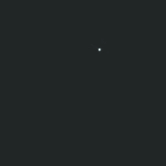
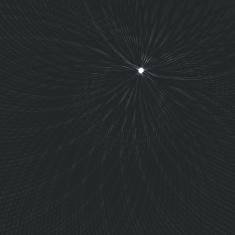
(a)	(b)	(c)

Figure 2: (a) Propagating acoustic front (b) the result of focusing at the point $(0.2,0.4)$ (c) same as (b) with the gray scale showing the lower $10\%$ of the range of the function

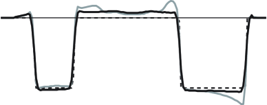
Figure 3: Horizontal central cross-section (accurate data): dashed line denotes the phantom, gray line represents iteration # 0, thick black solid line represents iteration #1

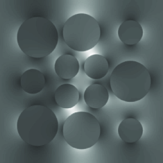
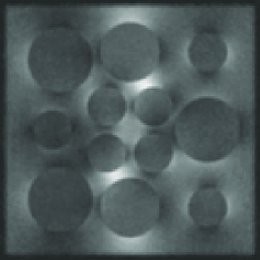
(a)	(b)
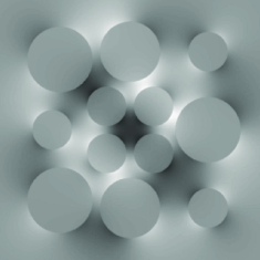
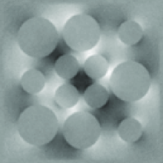
(c)	(d)

Figure 4: Functionals $M_{i,j}$: (a) original $M_{1,1}$ (b) $M_{1,1}$ reconstructed from data contaminated by $50\%$ noise (c) original $M_{1,2}$ (d) $M_{1,2}$ reconstructed from data contaminated by $50\%$ noise

4 Numerical examples in $2D$

We will now illustrate the properties of our algorithm on several numerical examples in $2D$. Each simulation involves several steps. First we model the direct problem as follows. For a given phantom of $\sigma$ and a fixed boundary current $J$ we solve equation (1) in the unit square $[-1,1]\times[-1,1]$, and (for a chosen weight function $I$) we compute the unperturbed boundary functionals $M^{\mathrm{unperturbed}}_{I,J}$:

$$M^{\mathrm{unperturbed}}_{I,J}:=\int\limits_{\partial\Omega}u(z)I(z)dz.$$ (24)

Next, for a set of values of $t$ and $z$ we perturb $\sigma$ by multiplying it by $\operatorname{exp}(\eta_{t,z}(x))$ with $\eta_{t,z}(x)$ proportional to the propagating acoustic pulse $W_{t,z}$ given by equation (7). (In simulation we used a mollified version of the delta-function, which corresponds to a transducer with a finite bandwidth.) For each perturbed $\sigma$ we again solve equation (1), obtain the solution $u^{\mathrm{perturbed}}$, and compute functionals

$$M^{\mathrm{perturbed}}_{I,J}(t,z):=\int\limits_{\partial\Omega}u^{\mathrm{perturbed}}(z)I(z)dz.$$ (25)

Finally, the difference of $M^{\mathrm{perturbed}}_{I,J}(t,z)$ and $M^{\mathrm{unperturbed}}_{I,J}$ yields the values of the functionals $M_{I,J}(t,z)$ given by equation (8) which we consider the simulated measurements and the starting point for solving the inverse problems. In some of our numerical experiments we add values of a random variable to these functions to simulate the noise in the measurements.

The advantage of computing $M_{I,J}(t,z)$ as the difference of two solutions (as opposed to obtaining it from the linearized equation (8)) consists in eliminating the chance of committing “an inverse crime”. However, since subtraction of two numerically computed functions that differ very little can significantly amplify the relative error, our forward solver has to be very accurate. In order to achieve high accuracy we approximated the potentials in the square by Fourier series and used the Fast Fourier transforms (FFT) to compute the corresponding differential operators. In turn, the application of the FFTs allowed us to use fine discretization grids ($513\times 513$), which, in combination with smoothing of the simulated $\sigma(x)$ yields the desired high accuracy. (Such algorithms combining the use of global bases (such as the trigonometric basis utilized here) with enforcing the equation in the nodes of the computational grid are called pseudospectral [11]; they are very efficient when the computational domain is simple (e.g. a square) and the coefficients of the equation are smooth.)

After the measurement data have been simulated, the inverse problem of AET is solved by reconstructing functions $M_{i,j}$ (see equation (9)) from $M_{I,J}(t,z)$ (synthesis step), and by applying the methods of Section 2 to reconstruct $\varepsilon\rho(x)$ (i.e. the difference between the true conductivity and the benchmark $\sigma_{0}$).

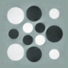
(a)	(b)	(c)

Figure 5: Reconstruction from the data contaminated by a $50\%$ noise (a) phantom (b) iteration #0 (c) iteration #1

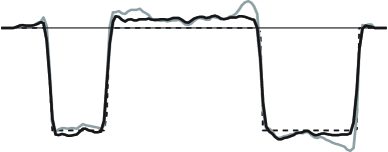
Figure 6: Horizontal central cross-section (noisy data): dashed line denotes the phantom, gray line represents iteration #0, thick black solid line represents iteration #1

Our phantom (i.e., simulated $\ln\sigma(x)$) consists of several slightly smoothed characteristic functions of circles, shown in Figure 1(a) and Figure 5(a). (A more detailed description is presented in the Appendix). Smoothing guarantees that the phantom is fully resolved on the fine discretization grid we use during the forward computations, which helps to ensure its high accuracy (several correct decimal digits). The characteristic functions comprising the phantom are weighted with weights 1 or -1, so that $\sigma(x)$ varies between $e$ and $e^{-1}$. Thus, the conductivity deviates far from the initial guess $\sigma_{0}\equiv 1$. Current $I_{1}$ equals $1$ and $-1$ on the right and left sides of square, respectively; it vanishes on the horizontal sides. Current $I_{2}$ coincides with $I_{1}$ rotated $90$ degrees counterclockwise.

The simulated sources of the propagating spherical acoustic fronts are centered on a circle of the diameter slightly larger than the diagonal of the square domain. There were $256$ simulated transducers uniformly distributed over the circle. Each transducer produced $257$ spherical fronts of the radii ranging from $0$ to the diameter of the circle. For each front radius $t_{l}$ and center $z_{m}$, the perturbed $\sigma$ was modeled, the non-linear direct $M_{I_{j},I_{k}}(t_{l},z_{m})$, $j,k=1,2$ were computed as explained at the beginning of this section. In the first of our experiments, these accurate data were used as a starting point of the reconstruction. In the second experiment, they were perturbed by a 50% (in the $L^{2}$ norm) noise.

(a)	(b)	(c)

Figure 7: Reconstruction from noiseless data (a) phantom (b) iteration #0 (c) iteration #4

The first step of the reconstruction is synthetic focusing, i.e. finding the values $M_{j,k}(x)$ from $M_{I_{j},I_{k}}(t,z)$, $j,k=1,2$. In order to give the reader a better feeling of synthetic focusing, we present in the Figure 2 a picture of a propagating spherical acoustic front (part (a)), and an approximation to a delta function located at the point $(0.2,0.4)$ obtained as a linear combination of such fronts (part (b)). Figure 2(c) shows the same function as in the part (b) with a modified gray scale that corresponds to the lower $10\%$ of that function’s range, and thus allow one to see small details invisible in part (b). These figures are provided for demonstration purposes only, since in our algorithm reconstruction of the values $M_{j,k}(x)$ from $M_{I_{j},I_{k}}(t,z)$ is done by applying the $2D$ exact filtration backprojection formula to the latter function (we used the exact reconstruction formula from [17], but other options are also available). On a $129\times 129$ grid this computation takes a few seconds. Since the formula is applied to the data containing the derivative of the delta-function, the differentiation appearing in the TAT inversion formula (e.g., [1, 15, 10, 17]) is not needed, and the reconstruction instead of being slightly unstable, has a smoothing effect (this is why we obtain high quality images with such high level of noise).

On the second step of the reconstruction, functions $M_{j,k}^{0}(x)$ are computed using the knowledge of the benchmark conductivity $\sigma_{0}$, and values of $g_{j,k}(x)$ are obtained by comparing $M_{j,k}(x)$ and $M_{j,k}^{0}(x)$. Then the first approximation to $\rho$ (we will call it iteration #0) is obtained by solving equation (21). The right hand side of this equation is computed by finite differences, and then the Poisson equation in a square is solved by the decomposition in $2D$ Fourier series. The computation is extremely fast due to the use of the FFT. More importantly, since the differentiation of the data is followed by the application of the inverse Laplacian, this step is completely stable (the corresponding pseudodifferential operator is of order zero), and no noise amplification occurs. Finally, we attempt to improve the reconstruction by accepting the reconstructed $\sigma$ as a new benchmark conductivity and by applying to the data the parametrix algorithm of the previous section. We will call this computation iteration #1. Figure 1 demonstrates the result of such reconstruction from data without noise. Part (a) of the Figure shows the phantom, parts (b) and (c) present the results of iterations #0 and #1, on the same gray-level scale. The profiles of the central horizontal cross-sections of these functions are shown in Figure 3. One can see that even the iteration #0 produces quite good a reconstruction; iteration #1 removes some of the artifacts, and improves the shape of circular inclusions. For the convenience of the reader we summarize the parameters of this simulation in the Appendix.

Figures 4, 5 and 6 present the results of the reconstruction from noisy data. In this simulation we used the phantom from the previous example, and we added to the data $50\%$ (in $L^{2}$ norm) noise. The first step of the reconstruction (synthetic focusing) is illustrated by Figure 4. Parts (a) and (c) of this Figure show accurate values of the functionals $M_{1,1}(x)$ and $M_{1,2}(x)$. Parts (b) and (d) present the reconstructed values of these functionals obtained by synthetic focusing. One can see the effect of smoothing mentioned earlier in this section: the level of noise in the reconstructions is much lower than the level of noise in the simulated measurements. The images reconstructed from $M_{i,j}(x)$ on the second step are presented in Figures 5 and 6. The meaning of the images is the same as of those in Figures 1 and 3. The level of noise in these images is comparable to that in the reconstructed $M_{i,j}$’s. To summarize, our method can reconstruct high quality images from the data contaminated by a strong noise since the first step of the method is an application of a smoothing operator, and the second step uses the parametrix.

Finally, Figure 7 shows reconstruction of a phantom containing objects with corners. The phantom is shown in the part (a) of the figure, part (b) demonstrates iteration #0, and part (c) presents the result of the iterative use of the parametrix method described in the previous section (iteration #4 is shown).

5 Reconstruction in $3D$

Let us now consider the reconstruction problem in $3D$. The $3D$ case is very important from the practical point of view, since propagation of electrical currents is essentially three-dimensional. Indeed, unlike X-rays or high-frequency ultrasound, currents cannot be focused to stay in a two-dimensional slice of the body. However, while successful $3D$ reconstructions were reported [7], the theoretical foundations of the $3D$ case have not been completed yet, due to some analytic difficulties arising in other approaches. In contrast, the present approach easily generalizes to $3D$, and leads to a fast, efficient, and robust reconstruction algorithm.

We will assume that three different currents $I_{j},j=1,2,3$ are used, and that the boundary values of the corresponding potentials $w_{j},$ $j=1,2,3$ are measured on $\partial\Omega.$ Similarly to the $2D$ case presented in Section 1, by perturbing the medium with a perfectly focused acoustic beam (no matter whether such measurements are real or synthesized) one can recover at each point $x$ within $\Omega$ the values of the functionals $M_{i,j}(x),$ $i,j=1,2,3,$ where, as before,

$$M_{i,j}(x)=\sigma(x)\nabla w_{i}(x)\cdot\nabla w_{j}(x).$$

Our goal is to reconstruct conductivity $\sigma(x)$ from $M_{i,j}(x).$ As before, we will assume that $\sigma(x)$ is a perturbation of a known benchmark conductivity $\sigma_{0}(x),$ i.e. $\sigma(x)=\sigma_{0}(x)(1+\varepsilon\rho(x)),$ and that the values of potentials $w_{j}(x)$ are the perturbations of known potentials $u_{j}(x)$ corresponding to $\sigma_{0}(x):$

$$w_{j}(x)=u_{j}(x)+\varepsilon v_{j}(x)+o(\varepsilon).$$

Now functionals $M_{j,k}(x)$ are related to the known unperturbed values $M_{j,k}^{0}(x)$ and measured perturbations $g_{j,k}(x)$ by equations (14) and (13).

As it was done in Section 2, we introduce vector fields $U_{j}=\sqrt{\sigma_{0}}\nabla u_{j}$ and $W_{j}=\sqrt{\sigma}\nabla(u_{j}+\varepsilon v_{j})=U_{j}+\varepsilon V_{j},$ and proceed to derive the following six equations:

$$U_{1}\cdot V_{1} =g_{1,1}/2$$

$$U_{2}\cdot V_{2} =g_{2,2}/2$$

$$U_{3}\cdot V_{3} =g_{3,3}/2$$

$$U_{1}\cdot V_{2}+U_{2}\cdot V_{1} =g_{1,2}$$

$$U_{1}\cdot V_{3}+U_{3}\cdot V_{1} =g_{1,3}$$

$$U_{2}\cdot V_{3}+U_{3}\cdot V_{2} =g_{2,3}.$$

One can obtain a useful approximation to $\rho(x)$ by assuming $\sigma_{0}=1$, and by selecting unperturbed currents so that the potentials $u_{j}(x)=x_{j}$. Then, by repeating derivations of Section 2.1 one obtains the following three formulas

$$\left\{\begin{array}[c]{c}\left(\frac{\partial^{2}}{\partial x_{1}^{2}}+\frac{\partial^{2}}{\partial x_{2}^{2}}\right)\rho=\frac{1}{2}\left(\frac{\partial^{2}}{\partial x_{1}^{2}}-\frac{\partial^{2}}{\partial x_{2}^{2}}\right)(g_{2,2}-g_{1,1})-2\frac{\partial^{2}}{\partial x_{1}\partial x_{2}}g_{1,2}\\ \left(\frac{\partial^{2}}{\partial x_{1}^{2}}+\frac{\partial^{2}}{\partial x_{3}^{2}}\right)\rho=\frac{1}{2}\left(\frac{\partial^{2}}{\partial x_{1}^{2}}-\frac{\partial^{2}}{\partial x_{3}^{2}}\right)(g_{3,3}-g_{1,1})-2\frac{\partial^{2}}{\partial x_{1}\partial x_{3}}g_{1,3}\\ \left(\frac{\partial^{2}}{\partial x_{2}^{2}}+\frac{\partial^{2}}{\partial x_{3}^{2}}\right)\rho=\frac{1}{2}\left(\frac{\partial^{2}}{\partial x_{2}^{2}}-\frac{\partial^{2}}{\partial x_{3}^{2}}\right)(g_{3,3}-g_{2,2})-2\frac{\partial^{2}}{\partial x_{2}\partial x_{3}}g_{2,3}\end{array}\right.$$ (26)

We notice that by using the first of the above equations one can compute an approximation to $\rho(x)$ by solving a set of $2D$ Poisson equations (one for each fixed value of $x_{3})$, since boundary values of $\rho(x)$ are equal to 0. This leads to a slice-by-slice $3D$ reconstruction, which is based only on values of $g_{1,1},$ $g_{2,2}$ and $g_{1,2}$, and therefore can be done by using a single pair of currents.

One can get better images by using all three currents and doing a fully $3D$ reconstruction. Namely, summing the equations (26) yields the values of $2\Delta\rho$ in the left hand side. Then one can solve the $3D$ Poisson equation with the zero boundary conditions to recover the conductivity.

One can expect that, as in $2D$, this approach would work well for $\sigma(x)$ close to $\sigma_{0}=1$. However, as demonstrated by our numerical experiments presented in Section 6, the results remain quite accurate when $\sigma(x)$ varies significantly across $\Omega$. Moreover, a simple fixed point iteration based on the repeated use of formulas (26) exhibits a rapid convergence to the correct image.

6 Numerical examples in $3D$

(a)	(b)	(c)

Figure 8: $3D$ Reconstruction from noiseless data. First row: phantom (a) $Ox_{1}x_{2}$ cross section (b) $Ox_{1}x_{3}$ cross section (c) $Ox_{2}x_{3}$ cross section. Second row: iteration #0; Third row: iteration #4

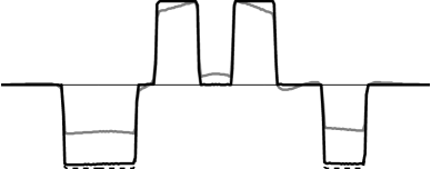
Figure 9: Diagonal cross-section (noiseless data): dashed line denotes the phantom, gray line represents iteration # 0, thick black solid line represents iteration #4

In this section we present results of $3D$ reconstructions from simulated data. Unfortunately, a complete modeling of the forward problem in $3D$ (i.e. computation of the perturbations corresponding to the propagating acoustic spherical fronts) would require solution of $\mathcal{O}(n^{3})$ $3D$ divergence equations. This task is computationally too expensive. Therefore, unlike in our $2D$ simulations, we resort to modeling the values of the functionals $M_{i,j}(x)$ on a $257\times 257\times 257$ Cartesian grid, using formulas (5). These values correspond to the data that would be measured if perfectly focused, infinitely small perturbations were applied to the conductivity. Thus, in this section we only test the second step of our reconstruction techniques. However, as mentioned before, if the real data were available, the first step (synthetic focusing) could be done by applying any of the several available stable versions of thermoacoustic inversion, and the feasibility of this step was clearly demonstrated in the $2D$ sections of this paper, as well as in [16].

In our first simulation we used noiseless values of $M_{i,j}(x)$ and reconstructed the conductivity on a $257\times 257\times 257$ grid. The first row of Figure 8 shows three $2D$ cross-sections of a $3D$ phantom. The result of approximate inversion (using three currents, as described in Section 5) is presented in the second row of the figure. Finally, the last row shows the result of iterative use of formulas (26), where $\rho$ now represents the difference between the previous and the updated approximations to the conductivity. The third row demonstrates iteration #4. In addition, Figure 9 shows the trace along a diagonal cross section in $Ox_{1}x_{2}$ plane (that corresponds to the diagonals of images presented in the column (a) of Figure 8). We summarize the details of this simulation in the Appendix.

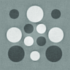
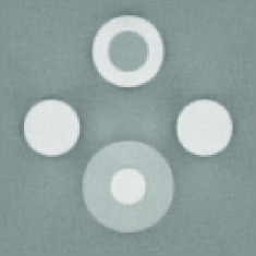
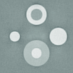
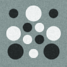
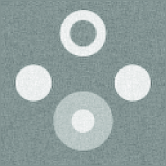
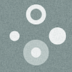
(a)	(b)	(c)

Figure 10: $3D$ Reconstruction from noisy data on a coarser grid. First row: phantom (a) $Ox_{1}x_{2}$ cross section (b) $Ox_{1}x_{3}$ cross section (c) $Ox_{2}x_{3}$ cross section. Second row: iteration #0; Third row: iteration #4

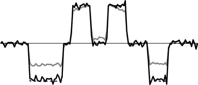
Figure 11: Diagonal cross-section of reconstructions obtained from noisy data on a coarser gird: dashed line denotes the phantom, gray line represents iteration # 0, thick black solid line represents iteration #4

In our second $3D$ experiment we utilized the same phantom, but as a data used only a subset of the values of $M_{i,j}$ corresponding to a coarser $129\times 129\times 129$ grid; the latter coarse grid was also used to discretize the reconstructed conductivity. We also added to the data a $10\%$ (in $L^{2}$ norm) noise. Figure 10 presents the cross-sections of a $3D$ phantom and the reconstructions obtained using three currents, on the same gray-level scale. The meaning of the subfigures is the same as of those in Figure 8. Finally, Figure 11 shows the trace along the diagonal cross sections of the images in the $Ox_{1}x_{2}y$ plane.

In both these examples iteration #0 yields good qualitative reconstruction of the conductivity in spite the fact that the latter varies from $e^{-1}$ to $e^{1}$, and thus differs strongly from the benchmark guess $\sigma_{0}=1$. The subsequent iterations demonstrate fast convergence to the correct values of $\sigma(x)$.

7 Final remarks and conclusions

We have shown that the proposed algorithm works stably and yields quality reconstructions of the internal conductivity. It does not require physical focusing of ultrasound waves and replaces it with the synthetic focusing procedure, which can be implemented using one of the known thermoacoustic imaging inversion methods (e.g., time reversal or inversion formulas). Under appropriate smoothness conditions on the conductivity, our analysis leads to the proof of local uniqueness and stability of the reconstruction. However, since this conclusion has been already made in $2D$ in [7, 5], we only presented a sketch of the proof.

Some additional remarks:

1. Using the propagating spherical fronts of the type considered in this text (equation (7)) is advantageous since in this case the synthetic focusing is a smoothing operator, and thus the whole reconstruction procedure is more stable with respect to errors than the one that starts with focused data.

2. Reconstructions can be done with a single, two, or (in $3D$) three currents. A single current procedure was the one we used initially in $2D$ [16, 18]. It works, but requires solving a transport equation for the conductivity. When such a procedure is used, errors arising due to the noise and/or underresolved interfaces tend to propagate along the current lines, thus reducing the quality of the reconstructed image. The two-current approach in $2D$ is elliptic and thus does not propagate errors. The two-current slice-by-slice reconstruction in $3D$ is also possible, but the use of three currents seem to produce better results.

The results of this work were presented at the conferences “Integral Geometry and Tomography”, Stockholm, Sweden, August 2008; “Mathematical Methods in Emerging Modalities of Medical Imaging”, BIRS, Banff, Canada, October, 2009; “Inverse Transport Theory and Tomography”, BIRS, Banff, May 2010; “Mathematics and Algorithms in Tomography” Oberwolfach (April 2010), and “Inverse problems and applications”, MSRI, Berkeley, August 2010. The brief reports have appeared in [16, 18].

$j$	$x_{j,1}$	$x_{j,2}$	$r^{\mathrm{out}}_{j}$	$r^{\mathrm{in}}_{j}$	$\alpha_{j}$
$1$	$-0.54$	$0.54$	$0.26$	$0.24$	$1$
$2$	$0.00$	$0.60$	$0.24$	$0.22$	$-1$
$3$	$0.60$	$0.60$	$0.16$	$0.14$	$1$
$4$	$-0.60$	$0.00$	$0.16$	$0.14$	$-1$
$5$	$0.60$	$0.00$	$0.26$	$0.24$	$-1$
$6$	$-0.54$	$-0.54$	$0.26$	$0.24$	$1$
$7$	$0.00$	$-0.60$	$0.24$	$0.22$	$-1$
$8$	$0.60$	$-0.60$	$0.16$	$0.14$	$1$
$9$	$0.18$	$0.18$	$0.16$	$0.14$	$-1$
$10$	$0.18$	$-0.18$	$0.16$	$0.14$	$1$
$11$	$-0.18$	$0.18$	$0.16$	$0.14$	$1$
$12$	$-0.18$	$-0.18$	$0.16$	$0.14$	$-1$

Table 1: Parameters of the $2D$ phantom

Appendix

In order to make it easier for the reader to repeat our simulations we summarize in this section the details of some of our numerical experiments.

In the first two of the $2D$ simulations described in Section 4 we use a $2D$ phantom in the form of a linear combination of twelve smoothed characteristic functions of disks with radii $r_{j}^{\mathrm{in}}$ and centers $x_{j}$:

$$f(x)=\sum_{j=1}^{12}\alpha_{j}h(|x-x_{j}|,r_{j}^{\mathrm{in}},r_{j}^{\mathrm{out}}),\quad x_{j}=(x_{j,1},x_{j,2}),$$

where

$$h(r,r_{j}^{\mathrm{in}},r_{j}^{\mathrm{out}})=\left\{\begin{array}[c]{ccc}1&,&r\leq r_{j}^{\mathrm{in}}\\ 0&,&r\geq r_{j}^{\mathrm{out}}\\ \exp\left[2\frac{r_{j}^{\mathrm{out}}-r_{j}^{\mathrm{in}}}{r-r_{j}^{\mathrm{out}}}\exp\left(\frac{r_{j}^{\mathrm{out}}-r_{j}^{\mathrm{in}}}{r_{j}^{\mathrm{in}}-r}\right)\right]&,&r_{j}^{\mathrm{in}}<r<r_{j}^{\mathrm{out}}\end{array}\right.,$$

and values of $\alpha_{j},$ $x_{j,1},$ $x_{j,2},$ $r_{j}^{\mathrm{in}},$ and $r_{j}^{\mathrm{out}}$ are given in Table 1. All the smoothed disks lie within the square computational domain $[-1,1]\times[-1,1]$. The forward problem was computed on a fine $513\times 513$ grid. We simulated propagating spherical fronts generated by $256$ transducers equally spaced on the circle of radius $1.6$ centered at the origin. For each transducer we simulated $257$ spherical fronts of varying radii. The reconstruction was performed on the coarser $129\times 129$ computational grid, from the data corresponding to two currents. In the first experiment we used the noiseless data, in the second one we added to the simulated values $M_{I,J}(t,z)$ values of a random variable modeling the noise of intensity $50\%$ of the signal in $L^{2}$ norm. The results of these simulations are described in Section 4.

In Section 6 we utilized a $3D$ phantom represented by a linear combination of sixteen smoothed characteristic functions of balls with radii $r_{j}^{\mathrm{in}}$ and centers $x_{j}$:

$$f(x)=\sum_{j=1}^{16}\alpha_{j}h(|x-x_{j}|,r_{j}^{\mathrm{in}},r_{j}^{\mathrm{out}}),\quad x_{j}=(x_{j,1},x_{j,2},x_{j,3}),;$$

the values of $\alpha_{j},$ $x_{j,1}$, $x_{j,2}$, $x_{j,3}$, $r_{j}^{\mathrm{in}}$, and $r_{j}^{\mathrm{out}}$ are given in Table 2. In our $3D$ simulations we had to assume that the values $M_{i,j}(x)$ are known. We modeled these values by using the above-mentioned phantom, in combination with three boundary current profiles. In the case of the constant conductivity these boundary currents would produce potentials equal to $x_{j}$, $j=1,2,3$. We modeled the direct problem using $257\times 257\times 257$ computational grid corresponding to the cube $[-1,1]\times[-1,1]\times[-1,1]$. In the first of our $3D$ experiments the reconstruction was done on the same grid from the noiseless data. In the second experiment the reconstruction was done on a coarser $129\times 129\times 129$ grid from the data contaminated by a $10\%$ noise (in $L^{2}$ norm). The results of these reconstructions are described in Section 6.

References

- [1] M. Agranovsky, P. Kuchment, and L. Kunyansky, On reconstruction formulas and algorithms for the thermoacoustic and photoacoustic tomography, Ch. 8 in L. H. Wang (Editor) ”Photoacoustic imaging and spectroscopy,” CRC Press 2009, pp. 89-101.
- [2] G. Alessandrini and V. Nesi, Univalent -harmonic mappings, Arch. Ration. Mech. Anal., 158 (2001), 155—171.
- [3] H. Ammari, E. Bonnetier, Y. Capdeboscq, M. Tanter, and M. Fink, Electrical impedance tomography by elastic deformation, SIAM J. Appl. Math. 68 (2008), 1557–1573.
- [4] D. C. Barber, B. H. Brown, Applied potential tomography, J. Phys. E.: Sci. Instrum. 17(1984), 723–733.
- [5] E. Bonnetier and F. Triki, A stability result for electric impedance tomography by elastic perturbation, Presentation at the workshop “Inverse Problems: Theory and Applications”, November 12th, 2010. MSRI, Berkeley, CA.
- [6] L. Borcea, Electrical impedance tomography, Inverse Problems 18 (2002), R99–R136.
- [7] Y. Capdeboscq, J. Fehrenbach, F. de Gournay, O. Kavian, Imaging by modification: numerical reconstruction of local conductivities from corresponding power density measurements, SIAM J. Imaging Sciences, 2/4 (2009), 1003–1030.
- [8] M. Cheney, D. Isaacson, and J.C. Newell, Electrical Impedance Tomography, SIAM Review, 41, No. 1, (1999), 85–101.
- [9] B. Cipra, Shocking images from RPI, SIAM News, July 1994, 14–15.
- [10] D. Finch and Rakesh, The spherical mean value operator with centers on a sphere, Inverse Problems 23 (2007), S37–S50.
- [11] B. Fornberg. A Practical Guide to Pseudospectral Methods. (Cambridge Monographs on Applied and Computational Mathematics, 1) Cambridge, Cambridge University Press 1996.
- [12] B. Gebauer and O. Scherzer, Impedance-Acoustic Tomography, SIAM J. Applied Math. 69(2): 565-576, 2009.
- [13] D. Gilbarg and N. S. Trudinger, Elliptic partial differential equations of second order, Reprint of the 1998 edition, Classics in Mathematics, Springer-Verlag, Berlin, 2001.
- [14] H. E. Hernandez-Figueroa, M. Zamboni-Rached, and E. Recami (Editors), ”Localized Waves”, IEEE Press, J. Wiley & Sons, Inc., Hoboken, NJ 2008.
- [15] P. Kuchment and L. Kunyansky, Mathematics of thermoacoustic tomography, European J. Appl. Math., 19 (2008), Issue 02, 191–224.
- [16] P. Kuchment and L. Kunyansky, Synthetic focusing in ultrasound modulated tomography, Inverse Problems and Imaging, 4 (2010), Number 4, 665 – 673.
- [17] L. A. Kunyansky, Explicit inversion formulae for the spherical mean Radon transform, Inverse Problems 23 (2007), pp. 373–383.
- [18] L. Kunyansky and P. Kuchment, Synthetic focusing in Acousto-Electric Tomography, in Oberwolfach Report No. 18/2010 DOI: 10.4171/OWR/2010/18, Workshop: Mathematics and Algorithms in Tomography, Organised by Martin Burger, Alfred Louis, and Todd Quinto, April 11th – 17th, 2010, pp. 44-47.
- [19] S. Lang, Introduction to Differentiable Manifolds, 2nd edition, Springer Verlag, NY 2002.
- [20] B. Lavandier, J. Jossinet and D. Cathignol, Quantitative assessment of ultrasound-induced resistance change in saline solution, Medical & Biological Engineering & Computing 38 (2000), 150–155.
- [21] B. Lavandier, J. Jossinet and D. Cathignol, Experimental measurement of the acousto-electric interaction signal in saline solution, Ultrasonics 38 (2000), 929–936.
- [22] V. S. Vladimirov Equations of mathematical physics. (Translated from the Russian by Audrey Littlewood. Edited by Alan Jeffrey.) Pure and Applied Mathematics, 3 Marcel Dekker, New York, 1971.
- [23] L. V. Wang and H. Wu, ”Biomedical Optics. Principles and Imaging”, Wiley-Interscience 2007.
- [24] M. Xu and L.-H. V. Wang, Photoacoustic imaging in biomedicine, Review of Scientific Instruments 77 (2006), 041101-01– 041101-22.
- [25] H. Zhang and L. Wang, Acousto-electric tomography, Proc. SPIE 5320 (2004), 145–149.