Large-deviation properties of largest component for random graphs

Abstract

Distributions of the size of the largest component, in particular the large-deviation tail, are studied numerically for two graph ensembles, for Erdős-Rényi random graphs with finite connectivity and for two-dimensional bond percolation. Probabilities as small as $10^{-180}$ are accessed using an artificial finite-temperature (Boltzmann) ensemble. The distributions for the Erdős-Rényi ensemble agree well with previously obtained analytical results. The results for the percolation problem, where no analytical results are available, are qualitatively similar, but the shapes of the distributions are somehow different and the finite-size corrections are sometimes much larger. Furthermore, for both problems, a first-order phase transition at low temperatures $T$ within the artificial ensemble is found in the percolating regime, respectively.

1 Introduction

For many problems in science and in statistics, the large deviation properties play an important role denHollander2000 ; dembo2010 . Only for few cases analytical results can be obtained. Thus, most problems have to be studied by numerical simulations practical_guide2009 , in particular by Monte Carlo (MC) techniques newman1999 ; landau2000 . Classically, MC simulation have been applied to random systems in the following way: For a finite set of independently drawn quenched random instances regular or large-deviation properties of these instances have been calculated using importance-sampling MC simulations. Only recently it has been noticed that by introducing an artificial sampling temperature also the large-deviation properties with respect to the quenched random ensemble can be obtained align2002 . This corresponds somehow to an annealed average, but the results are re-weighted in a way that the results for the original quenched ensemble are obtained. In this way, the large-deviation properties of the distribution of alignment scores for protein comparison was studied align2002 ; align_long2007 ; newberg2008 , which is of importance to calculate the significance of results of protein-data-base queries durbin2006 .

Motivated by these results, similar approaches have been applied to other problems like the distribution of the number of components of Erdős-Rényi (ER) random graphs rare-graphs2004 , the partition function of Potts models partition2005 , the distribution of ground-state energies of spin glasses pe_sk2006 and of directed polymers in random media monthus2006 , the distribution of Lee–-Yang zeros for spin glasses matsuda2008 , the distribution of success probabilities of error-correcting codes iba2008 , the distribution of free energies of RNA secondary structures rnaFreeDistr2010 , and some large-deviation properties of random matrices driscoll2007 ; saito2010 .

Interestingly, so far no comparison between numerical and mathematically exact results for the full support of a distribution involving a large-deviation tail has been performed to the knowledge of the author. In few cases, numerical results had been compared to rigorous results monthus2006 , but only near the peak of the distribution, where finite-size effects are often very small. In another case rare-graphs2004 , the numerical and analytical distributions were compared on the full support, but the result was obtained using a non-rigorous statistical mechanics approach. In this work, the numerical large-deviation approach is applied to obtain the complete distribution of the size $S$ of the largest component of ER random graphs. In this case also mathematically exact results for the leading order large-deviation rate function are available for arbitrary values of the finite connectivity $c$. This allows for a comprehensive comparison and an estimation of the strength of finite-size effects. Furthermore, in this paper results are obtained for the two-dimensional (2d) percolation problem, where no analytic results are available for the distribution of the largest-component size $S$. For both models also the dependence of $S$ on the artificial sampling temperature $T$ is studied. First-order phase transitions are found for both graph ensembles in the percolating regime.

The two graph ensembles are defined as follows. In both cases, each graph $G=(V,E)$ consists of $N$ nodes $i\in V$ and undirected edges $\{i,j\}\in E\subset V^{(2)}$. For ER random graphs erdoes1960 , each possible edge $\{i,j\}$ is present with probability $c/N$. Hence, the average degree (connectivity) is $c$. For 2d percolation, the graph is embedded in a two-dimensional square lattice of size $N=L\times L$ with periodic boundary conditions in both directions, i.e., in a torus. Each node can be connected by edges to its four nearest neighbours, each edge is present with probabilty $p$. Hence, the average deegree is $4p$.

Two nodes $i,j$ are called connected if there exist a path of disjoint edges $\{i_{0},i_{1}\},\{i_{1},i_{2}\},\ldots,\{i_{l-1},i_{l}\}$ such that $i=i_{0}$ and $j=i_{l}$. The maximum-size subsets $C\subset V$ of nodes, such that all pairs $i,j\in C$ are connected are called the (connected) components of a graph. The size of the largest component of a graph is denoted here by $S$. Via the random-graph enembles, a probability distribution $P(S)$ for the size of the largest component and the corresponding probability $P(s)$ for relative sizes $s=S/N$ are defined. The probabilities $P(s)$ for values of $s$ different from the typical size are exponentiall small in $N$. Hence, one uses the concept of the large-deviation rate function denHollander2000 by writing

$$P(s)=e^{-N\Phi(s)+o(N)}\quad(N\to\infty)$$ (1)

This leading-order behavior of the large-deviation rate function $\Phi_{\rm ER}(s,c)$ for ER random graphs with connectivity $c$ is known exactly biskup2007 and given by the following set of equations

$$\tilde{S}(s) = s\log s+(1-s)\log(1-s)$$

$$\pi_{1}(\alpha) = 1-e^{-\alpha}$$

$$\Psi(\alpha) = \left(\log\alpha-0.5[\alpha-1/\alpha]\right)\wedge 0$$

$$\Phi_{\rm ER}(s,c) = \tilde{S}(s)-s\log\pi_{1}(cs)-(1-s)\log\left(1-\pi_{1}(cs)\right)$$ (2)

$$-(1-s)\Psi\left(c(1-s)\right)\;,$$

where the expression $g(\alpha)\wedge 0$ results in 0 if $g(\alpha)>0$ and in $g(\alpha)$ else.

For percolation in finite dimensions similar results are not available, to the knowledge of the author. There are only analytical results for the distribution of finite (non-percolating) components alexander1990 .

The paper is organised as follows. In the second section, the numerical simulation technique and the corresponding re-weighting approach are explained. In the third section, the results are displayed, first for the ER random graph ensemble, next for the 2d percolation problem. Finally, a summary and an outlook are given. A concise summary of this paper is available at the papercore web page papercore .

2 Simulation and reweighting method

To determine the distribution $P(S)$ for any measurable quantity $S$, here denoting the largest component for an ensemble of graphs, simple sampling is straightforward: One generates a certain number $K$ of graph samples and obtains $S(G)$ for each sample $G$. This means each graph $G$ will appear with its natural ensemble probability $Q(G)$. The probability to measure a value of $S$ is given by

$$P(S)=\sum_{G}Q(G)\delta_{S(G),S}$$ (3)

Therefore, by calculating a histogram of the values for $S$, a good estimation for $P(S)$ is obtained. Nevertheless, $P(S)$ can only be measured in a regime where $P(S)$ is relatively large, about $P(S)>1/K$. Unfortunately, the distribution decreases exponentially fast in the system size $N$ when moving away from its typical (peak) value. This means, even for moderate system sizes $N$, the distribution will be unknown on almost its complete support.

To estimate $P(S)$ for a much larger range, even possibly on the full support of $P(S)$, where probabilities smaller than $10^{-100}$ may appear, a different approach is used align2002 . For self-containedness, the method is outlined subsequently. The basic idea is to use an additional Boltzmann factor $\exp(-S(G)/T)$, $T$ being a “temperature” parameter, in the following manner: A standard Markov-chain MC simulation newman1999 ; landau2000 is performed, where in each step $t$ from the current graph $G(t)$ a candidate graph $G^{*}$ is created: A node $i$ of the current graph is selected randomly, with uniform weight $1/N$, and all adjacent edges are deleted. For all feasible edges $\{i,j\}$, the edge is added with a weight corresponding to the natural weight $Q(G)$, i.e., with probability $c/N$ (ER random graph) or with probability $p$ (percolation), respectively. For the candidate graph, the size $S(G^{*})$ of the largest component is calculated. Finally, the candidate graph is accepted, ($G(t+1)=G^{*}$) with the Metropolis probability

$$p_{\rm Met}=\min\left\{1,e^{-[S(G^{*})-S(G(t))]/T}\right\}\,.$$ (4)

Otherwise the current graph is kept ($G(t+1)=G(t)$). By construction, the algorithm fulfills detailed balance. Clearly the algorithm is also ergodic, since within $N$ steps, each possible graph may be constructed. Thus, in the limit of infinite long Markov chains, the distribution of graphs will follow the probability

$$q_{T}(G)=\frac{1}{Z(T)}Q(G)e^{-S(G)/T}\,,$$ (5)

where $Z(T)$ is the a priori unknown normalisation factor.

The distribution for $S$ at temperature $T$ is given by

$$P_{T}(S) = \sum_{G}q_{T}(G)\delta_{S(G),S}$$

$$\stackrel{{\scriptstyle(\ref{eq:qT})}}{{=}} \sum_{G}Q(G)e^{-S(G)/T}\delta_{S(G),S}$$

$$= \frac{e^{-S/T}}{Z(T)}\sum_{G}Q(G)\delta_{S(G),S}$$

$$\stackrel{{\scriptstyle(\ref{eq:PS})}}{{=}} \frac{e^{-S/T}}{Z(T)}P(S)$$

$$\Rightarrow\quad P(S) = e^{S/T}Z(T)P_{T}(S)$$ (6)

Hence, the target distribution $P(S)$ can be estimated, up to a normalisation constant $Z(T)$, from sampling at finite temperature $T$. For each temperature, a specific range of the distribution $P(S)$ will be sampled: Using a positive temperature allows to sample the region of a distribution left to its peak (values smaller than the typical value), while negative temperatures are used to access the right tail. Temperatures of large absolute value will cause a sampling of the distribution close to its typical value, while temperatures of small absolute value are used to access the tails of the distribution. Hence, by choosing a suitable set of temperatures, $P(S)$ can be measured over a large range, possibly on its full support.

The normalisation constants $Z(T)$ can easily be obtained by including a histogram obtained from simple sampling, which corresponds to temperature $T=\pm\infty$, which means $Z\approx 1$ (within numerical accuracy). Using suitably chosen temperatures $T_{+1}$, $T_{-1}$, one measures histograms which overlap with the simple sampling histogram on its left and right border, respectively. Then the corresponding normalisation constants $Z(T_{\pm 1})$ can be obtained by the requirement that after rescaling the histograms according to (6), they must agree in the overlapping regions with the simple sampling histogram within error bars. This means, the histograms are “glued” together. In the same manner, the range of covered $S$ values can be extended iteratively to the left and to the right by choosing additional suitable temperatures $T_{\pm 2},T_{\pm 3},\ldots$ and gluing the resulting histograms one to the other. A pedagogical explanation and examples of this procedure can be found in Ref. align_book .

In order to obtain the correct result, the MC simulations must be equilibrated. For the case of the distribution of the size of the largest component, this is very easy to verify: The equilibration of the simulation can be monitored by starting with two different initial graphs, respectively:

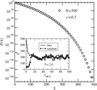
• Either an unbiased random graph is taken, which means that the largest component is of typical size. In the inset of Fig. 1 the evolution of $S$ as a function of the number $t_{\rm MCS}=t/N$ of Monte Carlo sweeps is shown for Erdős-Rény random graphs with $N=500$ nodes, connectivity $c=0.5$ at temperature $T=2$. As one can see, $S(t_{\rm MCS})$ moves quickly away from the typical size which is around $S=30$ towards a values around $S=200$. This shows that easily different parts of the distribution can be addressed. The result of a second run with a negative temperature is shown in the same inset. In this case an initial graph was used which consists of a single line of nodes, i.e., in particular the graph is fully connected leading to $S=N$.

• Alternatively, if the temperature is positive, one can start with an empty graph ($S=1$). In any case, for the two different initial conditions, the evolution of $S(t_{\rm MCS})$ will approach from two different extremes, which allows for a simple equilibration test: equilibration is achieved if the measured values of $S$ agree within the range of fluctuations. Only data was used in this work, where equilibration was achieved within 200 Monte Carlo steps.

The resulting distribution for ER random graphs ($C=2,N=500$) is shown in the main plot of Fig. 1. As one can see, the distribution can be measured over its full support such that probabilities as small as $10^{-180}$ are accessible.

Figure 1: Distribution of the size $S$ of the largest component for Erdős-Rényi random graphs of size $N=500$ at connectivity $c=0.5$. In this and all other plots, error bars are of symbol size or smaller if not explicitly shown. The inset shows the size of the largest component as function of the number $t_{\rm MCS}$ of Monte Carlo sweeps for the same type of graphs at temperature $T=-2$. Two different starting conditions are displayed: either a random graph (leading to a typical components size around $30$) or a graph consisting of a line $(S=500)$ were used.

Note that in principle one can also use a Wang-Landau approach wang2001 or similar approaches to obtain the distribution $P(S)$ without the need to perform independent simulations at different values for the temperatures. Nevertheless, the author has performed tests for ER random graphs and experienced problems by using the Wang-Landau approach, because the sampled distributions tend to stay in a limited fraction of the values of interest. Using the finite-temperature approach it is much easier to guide the simulations to the regions of interest, e.g., where data is missing using the so-far-obtained data, and to monitor the equilibration process. Furthermore, the behavior of $S$ as a function of $T$ appears to be of interest on its own, see next section.

3 Results

ER random graphs of size $N=500$ and 2d percolation problems with lateral size $L=32$ ($N=1024$ sites) were studied. In few cases, additional system sizes were considered to estimate the strength of finite-size effects, see below. For each problem, the model was studied right at the percolation transition, for one point in the non-percolating regime, and for one point in the percolating regime. The temperature ranges used for the different cases are shown in Tab. 1. Note that, depending on the position of the peak of the size distribution, sometimes positive, sometimes negative and sometimes both types of temperatures had to be used. For the systems listed in the table, equilibration was always achieved within the first 200 MCS. In general, studying significantly larger sizes or going deeper into the percolation regime makes the equilibration much more difficult. After equilibration, data was collected for 9800 MCS, in some cases, to improve statistics, for about $10^{6}$ MCS. In the two subsequent subsections, the results for ER random graphs and for 2d percolation are presented, respectively.

system	$T_{1}$	$T_{2}$	$N_{T}$
ER $c=0.5$	-5	-0.4	14
ER $c=1.0$	-7.0	-0.6	9
ER $c=2.0$	-2.0	10.0	6
perc $p=0.3$	-10.0	-0.6	13
perc $p=0.5$	-5.00	50.0	13
perc $p=0.6$	0.60	30.0	14

Table 1: Parameters used to determine the distributions $P(S)$ for the different models. $T_{1}$ is the minimum and $T_{2}$ the maximum temperature used. $N_{T}$ denotes the number of different temperature values. Note that for determinining the average value $\overline{S}(T)$, see Figs. 4 and 9, usually a higher number of temperatures was used.

3.1 ER graphs

For the numerical simulations, first the case of ER random graphs is treated, because the analytical result (2) can be used for comparison. This allows to assess the quality of the method and to get an impression of influence of the non-leading finite-size corrections.

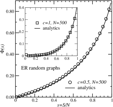
In Fig. 2 the empirical rate function

$$\Phi(s)\equiv-\frac{1}{N}\log P(s)$$ (7)

for $c=0.5$ is displayed, corresponding to the distribution shown in Fig. 1. Note that by just stating the analytical asymptotic rate function $\Phi_{\rm ER}(s,c)$, the corresponding distribution $P(s)$ is not normalised. Hence, for comparison, $\Phi(s)$ is shifted for all values of the connectivity $c$ such that it is zero at its minimum value, like $\Phi_{\rm ER}(s,c)$.

The numerical data agrees very well with the analytic result. Only in the region of intermediate cluster sizes, a small systematic deviation is visible, which is likely to be a finite-size effect. Given that for the numerical simulations only graphs with $N=500$ nodes were treated, the agreement with the $N\to\infty$ leading-order analytical result is remarkable.

The resulting rate function right at the percolation transition $c=c_{\rm c}=1$ is shown in the inset of Fig. 2. Qualitatively, the result is very similar to the non-percolating case $c=0.5$, except that the distribution is much broader, corresponding to smaller values of the rate function. Again, the agreement with the analytical result is very good, except for the data close to the origin $s=0$: The numerical results exhibit a minimum near $s=0.05$, while the analytical result exhibits its minimum naturally at $s=0$. This is clearly due to the finite size of the numerical samples.

Figure 2: Large-deviation rate function $\Phi(s)$ of ER random graphs with average connectivity $c=0.5<c_{\rm c}$, $N=500$ (symbols). The line displays the analytical result from Eq. (2). The inset shows the same for the case $c=1.0=c_{\rm c}$.

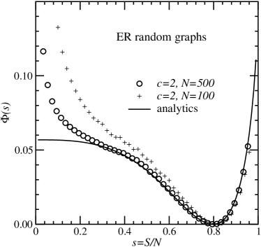
The case of the percolating regime (connectivity $c=2$), is displayed in Fig. 3. The rate function exhibits a minimum at a finite value of $s$, corresponding to the finite average fraction of nodes contained in the largest component. The behaviour of the rate function is more interesting compared to $c\leq c_{\rm c}$, because $\Phi_{\rm ER}(s)$ grows strongly near its minimum, but for $s\to 0$ it levels off horizontally. For most of the support of the distribution, the numerical data for $N=500$ agrees again very well with the analytic result. Nevertheless, for $s\to 0$, strong deviations become visible because the numerical rate function $\Phi(s)$ grows strongly as $s\to 0$. By comparing with the result for a smaller system, $N=100$, where this deviation is even larger, it becomes clear that this is a finite-size effect, corresponding to the non-leading corrections, which will disappear for $N\to\infty$.

Figure 3: Large-deviation rate function $\Phi(s)$ of ER random graphs with average connectivity $c=2>c_{\rm c}$, $N=100$ and $N=500$ (symbols). The line displays the analytical result from Eq. (2).

Although the parameter $T$ is mainly used as a way to address different parts of the distribution, the temperature dependence of $S$, which is shown in Fig. 4, exhibits an interesting behaviour on its own in the percolating regime. When studying the average size $\overline{s}$ as a function of temperature, a strong increase around temperature $T=9.5$ becomes visible, which may correspond to a kind of phase transition, see below.

Figure 4: Average relative size $\overline{s}$ of the largest component as a function of artificial temperature $T$ for ER random graphs in the percolating regime ($c=2$) and (inset) in the non-percolating regime ($c=0.5$).

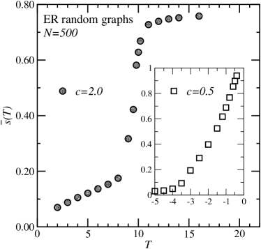
On the other hand, in the non-percolating regime $c<1$, the average size of the largest component is rather smooth, as shown in the inset of Fig. 4. Note that here negative artificial temperatures are used, because the peak of the distribution $P(S)$ is close to $S=0$, in contrast to the percolating regime $c>1$, where the peak of $P(S)$ is at finite values.

In Fig. 5 the size $S$ of the largest component is shown as a function of the number of MC sweeps for a temperature $T=9.5$, which is located in the regime of the assumed transition. One can see that $S(t)$ fluctuates quickly between two sets of typical sizes, which shows also that the data is well equilibrated. In particular, values around $S=350$ and around $S=100$ are more frequent than intermediate values.

Figure 5: Time-series for the size $S$ of largest cluster as function of the number $t_{\rm MCS}$ of MC sweeps for ER random graphs ($c=2$, $N=500$) at artificial temperature $T=9.5$.

This result is made more quantitative by studying the resulting distribution of the sizes of the largest component, see Fig. 6. A two-peak structure can be observed, which indicates that indeed a transition between small and large components of first-order type is present in the percolating regime $c>1$. Similar first-order transitions have been observed for biased simulations of the one-dimensional Ising model jack2010 ; jack2010b . The first-order nature of this transition is a reason that obtaining $\Phi(s)$ becomes harder for large system sizes, because the time for tunnelling between the two sets of values grows quickly. Furthermore, even worse, the number of observed configurations having a value of $S$ which is located between the peaks decreases strongly, such that for large intervals no data can be collected at all, already for $N=1000$. Hence, $P(S)$ cannot be sampled for such system sizes on its complete support, because the different parts of the distribution cannot be “glued” together.

Figure 6: Distribution (normalised such that the integral is one) of the size of the largest component for ER random graphs ($c=2$, $N=500$) at artificial temperature $T=9.5$.

A detailed study of this phase transition is beyond the scope of this work, in particular because its physical relevance is yet not fully clear.

3.2 Two-dimensional percolation

Again the discussion of the rate function for the distribution of the relative size $s=S/N$ of the largest component is started by considering the non-percolating regime. The rate function for $p=0.3<p_{\rm c}$ ($L=32$) is shown in Fig. 7. In principle it looks similar to the ER case displayed in Fig. 2. A striking difference is that it exhibits a large region where it behaves linearly, basically for half of the support, while it grows stronger for $s>0.5$. For $L=16$ (not shown), the same result was found. This means, the finite-size effects are small as in the ER case. This also indicates that the shape of the rate function should basically remain the same for $L\to\infty$. In particular, it appears likely that for $L\to\infty$, $\Phi(s)$ will consist of a linear part for small values of $s$ and it will grow stronger for $s\to 1$.

Figure 7: Large-deviation rate function $\Phi(s)$ of two-dimensional (2d) bond percolation with occupation probability $p=0.3<p_{\rm c}$, $L=32$ (symbols). For small relative cluster sizes $s$, the rate function behaves linearly (the line displays a linear function with slope $0.1125$, obtained from fitting a linear function to the data in the range $s\in[0,0.5]$).

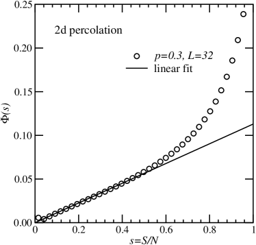
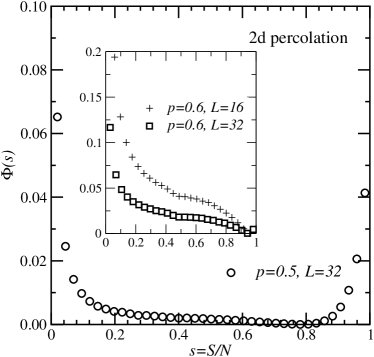
In contrast, the large-deviation rate function right at the percolation transition $p=p_{\rm c}=0.5$ ($L=32$), see Fig. 8, looks very different from the ER case: It exhibits a minimum at a relative cluster size of about $s=S/N=0.78$, see main plot in Fig. 8. This is very large compared to the ER case, but only a finite-size effect: For example for $L=512$ (additional simple sampling simulations, not shown), the minimum of the rate function has already moved to a smaller value of $s\approx 0.5$ and for $p=0.49$, just before the percolation transition, the most likely relative size of a cluster is $s=0.1$. Hence, the finite-size effects, i.e., corrections to the large-deviation rate function, are close to $p_{c}$ much stronger for the finite-dimensional case compared to ER random graphs.

The case of the percolating regime is displayed in the inset of Fig. 8. Here again, the result looks very similar to the ER case, except that the magnitude of the rate function is somehow smaller. Hence, it appears likely that the shape of the rate function for the 2d percolation problem in the limit $L\to\infty$ is very similar to the ER case, i.e., it may level off horizontally for $s\to 0$ at a finite value and the strong increase found for $L=32$ is again a finite size effect. This is confirmed by the result for $L=16$, which exhibits a much stronger increase for $s\to 0$ compared to the $L=32$ result, as in the case of ER random graphs.

Figure 8: Large-deviation rate function $\Phi(s)$ of two-dimensional (2d) bond percolation with occupation probability $p=0.5=p_{\rm c}$, $L=32$ and (inset) $p=0.6$, $L=16$/$L=32$.

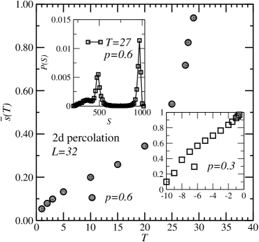
In Fig. 9 the result for the behaviour of $S$ as a function of the artificial temperature is shown. In the non-percolating regime ($p=0.3$), see right inset, the average value $\overline{s}$ behaves very regularly as a function of the temperature, no sign of a transition is visible. On the other hand, inside the percolation regime ($p=0.6$), see main plot, $\overline{s}(T)$ exhibits a strong increase around $T=27$. The distribution of $S$ at $T=27$ exhibits a strong bimodal signature, which indicates that indeed a phase transition of first-order type takes place. In summary, the temperature dependence of the size of the largest component is very similar to the results obtained for the ER random graphs.

Figure 9: Average relative size $\overline{s}$ of the largest component as a function of artificial temperature $T$ for 2d percolation ($L=32$) in the percolating regime ($p=0.6$) and (right inset) in the non-percolating regime ($p=0.6$). The left inset shows the distribution (normalised such that the integral is one) of the size of the largest component ($p=6$) at artificial temperature $T=27$ (line is guide to the eyes only).

4 Summary and outlook

By using an artificial Boltzmann ensemble characterised by an artificial temperature $T$, the distributions of the size of the largest component for ER randoms graphs with finite connectivity $c$ and for 2d percolation have been studied in this work. For not too large system sizes, the distributions can be calculated numerically over the full support, giving access to very small probabilities such as $10^{-180}$.

For the ER case, the numerical results for the large-deviation rate function $\Phi(s)$, obtained for rather small graphs of size $N=500$, agree very well with analytical results obtained previously for the leading behaviour in the limit $N\to\infty$. This proves the usefulness of the numerical approach, which has been applied previously to models where no complete comparison between numerical data and exact analytic results have been performed. The main findings are that below and at the percolation transition, $\Phi(s)$ exhibits a minimum at $s=0$ and rises monotonously for $s\to 1$. Inside the percolating regime, $\Phi(s)$ exhibits a minimum, grows quickly around this minimum and levels off horizontally for $s\to 0$. The finite-size corrections are usually small, except for the percolating regime in an extended region near $s=0$. Furthermore, when studying the average value $\overline{s}$ as a function of temperature, a transition of first-order type is found between a phase where $S$ is untypically small to a phase where $S$ is large.

For the 2d percolation problem, where no analytic results are available, basically the same results are found: the shape of the large-deviation rate functions below, at, and above the percolation threshold are qualitatively the same, except that the finite-size corrections at the percolation threshold appear to be larger compared to the ER results. Also the behaviour of the largest-component size as a function of the temperature seems to be similar, in particular exhibiting a first-order type transition for the percolating regime.

Since the comparison with the exact results for the ER random graphs indicates the usefulness of this approach to study large-deviation properties of random graphs, it appears promising to consider many other properties of different ensembles of random graphs in the same way. For example, it would be interesting to obtain the distribution of the diameter of ER random graphs, where only for $c<1$ there is an analytic result available. Corresponding simulations are currently performed by the author of this work.

References

- (1) F. den Hollander, Large Deviations (American Mathematical Society, Providence, 2000)
- (2) A. Dembo, O. Zeitouni, Large Deviations Techniques and Applications (Springer, Berlin, 2010)
- (3) A.K. Hartmann, Practical Guide to Computer Simulations (World Scientific, Singapore, 2009)
- (4) M.E.J. Newman, G.T. Barkema, Monte Carlo Methods in Statistical Physics (Clarendon Press, Oxford, 1999)
- (5) D.P. Landau, K. Binder, Monte Carlo Simulations in Statistical Physics (Cambridge University Press, Cambridge, 2000)
- (6) A.K. Hartmann, Phys. Rev. E 65, 056102 (2002)
- (7) S. Wolfsheimer, B. Burghardt, A.K. Hartmann, Algorithms for Molecular Biology 2, 9 (2007)
- (8) L. Newberg, J. Comp. Biol. 15, 1187 (2008)
- (9) R. Durbin, S.R. Eddy, A. Krogh, G. Mitchison, Biological Sequence Analysis (Cambridge University Press, Cambridge, 2006)
- (10) A. Engel, R. Monasson, A.K. Hartmann, J. Stat. Phys. 117, 387 (2004)
- (11) A. Hartmann, Phys. Rev. Lett. 94, 050601 (2005)
- (12) M. Körner, H.G. Katzgraber, A.K. Hartmann, JSTAT 2006(04), P04005 (2006), http://stacks.iop.org/1742-5468/2006/i=04/a=P04005
- (13) C. Monthus, T. Garel, Phys. Rev. E 74(5), 051109 (2006)
- (14) Y. Matsuda, H. Nishimori, K. Hukushima, J. Phys. A: Math. Theor. 41(32), 324012 (2008), http://stacks.iop.org/1751-8121/41/i=32/a=324012
- (15) Y. Iba, K. Hukushima, J. Phys. Soc. Japan 77(10), 103801 (2008), http://jpsj.ipap.jp/link?JPSJ/77/103801/
- (16) S. Wolfsheimer, A.K. Hartmann, Phys. Rev. E 82, 021902 (2010)
- (17) T.A. Driscoll, K.L. Maki, SIAM Review 49(4), 673 (2007), http://link.aip.org/link/?SIR/49/673/1
- (18) N. Saito, Y. Iba, K. Hukushima, Phys. Rev. E 82(3), 031142 (2010)
- (19) P. Erdős, A. Rényi, Publ. Math. Inst. Hungar. Acad. Sci. 5, 17 (1960)
- (20) M. Biskup, L. Chayes, S.A. Smith, Rand. Struct. Alg. 31, 354 (2007)
- (21) K. Alexander, J.T. Chayes, L. Chayes, Commun. Math. Phys. 131, 1 (1990)
- (22) Papercore is a free and open-access database for summaries of scientific (currently mainly physics) papers, http://www.papercore.org/Hartmann2010
- (23) A.K. Hartmann, in New Optimization Algorithms in Physics, edited by A.K. Hartmann, H. Rieger (Whiley-VCH, Weinheim, 2004), p. 253
- (24) F. Wang, D.P. Landau, Phys. Rev. Lett. 86, 2050 (2001)
- (25) R.L. Jack, P. Sollich, Prog. Theor. Phys. Supp. 184, 304 (2010)
- (26) R.L. Jack, private communication (2010)