Beyond pressureless gas dynamics : Quadrature-based velocity moment models

Christophe Chalons Université Paris Diderot-Paris 7 & Laboratoire J.-L. Lions, U.M.R. 7598 UMPC, Boîte courrier 187, 75252 Paris Cedex 05, France and Laboratoire EM2C - UPR CNRS 288, Ecole Centrale Paris, Grande Voie des Vignes, 92295 Chatenay-Malabry Cedex (chalons@math.jussieu.fr). This research was partially supported by an ANR Young Investigator Award (French Agence Nationale de la Recherche), contract ANR-08-JCJC-0132-01 - INTOCS - 2009-2013    Damien Kah Laboratoire EM2C - UPR CNRS 288, Ecole Centrale Paris, Grande Voie des Vignes, 92295 Chatenay-Malabry Cedex and IFP Energies Nouvelles, (damienk@stanford.edu). D. Kah was funded during his Ph.D. Thesis by an IFPEN/EM2C CIFRE Ph.D. Grant.    Marc Massot Laboratoire EM2C - UPR CNRS 288, Ecole Centrale Paris, Grande Voie des Vignes, 92295 Chatenay-Malabry Cedex (marc.massot@ecp.fr - Corresponding author. Present address : mmassot@stanford.edu - Center for Turbulence Research, Stanford University). This research was supported by an ANR Young Inverstigator Award for M. Massot, ANR-05-JCJC-0013 - jéDYS - 2005-2009. We would like to thank the Center for Turbulence Research at Stanford University and its director, Parviz Moin, for their kind invitation during the Summer Program 2010 where the present work was completed and Laboratory EM2C for supporting the visit of C. Chalons at Stanford as well as Damien Kah’s Master Thesis during which the study was initiated.
Abstract

Following the seminal work of F. Bouchut on zero pressure gas dynamics, extensively used for gas particle-flows, the present contribution investigates quadrature-based velocity moments models for kinetic equations in the framework of the infinite Knudsen number limit, that is, for dilute clouds of small particles where the collision or coalescence probability asymptotically approaches zero. Such models define a hierarchy based on the number of moments and associated quadrature nodes, the first level of which leads to pressureless gas dynamics. We focus in particular on the four moment model where the flux closure is provided by a two-node quadrature in the velocity phase space and provides the right framework for studying both smooth and singular solutions. The link with both the kinetic underlying equation as well as with zero pressure gas dynamics, i.e. the dynamics at the frontier of the moment space of order four, is provided. We define the notion of measure solutions and characterize the mathematical structure of the resulting system of four PDEs. We exhibit a family of entropies and entropy fluxes and define the notion of entropic solution. We study the Riemann problem and provide entropic solutions in particular cases. This leads to a rigorous link with the possibility of the system of macroscopic PDEs to allow particle trajectory crossing (PTC) in the framework of smooth solutions. Generalized δ𝛿\delta-shock solutions resulting from Riemann problem are also investigated. Finally, using a kinetic scheme proposed in the literature in several areas, we validate such a numerical approach and propose a dedicated extension at the frontier of the moment space in the framework of both regular and singular solutions. This is a key issue for application fields where such an approach is extensively used.

keywords:
Quadrature-based moment methods; gas-particle flows; kinetic theory; particle trajectory crossing; entropic measure solution; frontier of the moment space
subject classifications 76N15 (35L65 65M99 76M25 82C40).

1 Introduction

The physics of particles and droplets in a carrier gaseous flow field are described in many applications (fluidized beds, spray dynamics, alumina particles in rocket boosters, \dots) by a number density function (NDF) satisfying a kinetic equation introduced by [Williams (1958)]. Solving such a kinetic equation relies either on a sample of discrete numerical parcels of particles through a Lagrangian–Monte-Carlo approach or on a moment approach resulting in a Eulerian system of conservation laws on velocity moments eventually conditioned on size. In the latter case investigated in the present contribution, the main difficulty for particle flows with high Knudsen numbers (i.e. weakly collisional flows), where the velocity distribution can be very far from equilibrium, is the closure of the convective transport at the macroscopic level. One way to proceed is to use quadrature-based moment methods where the higher-order moments required for closure are evaluated from the lower-order transported moments using quadratures in the form of a sum of Dirac delta functions in velocity phase space (see [Yuan & Fox (2010), Kah (2010)] and the references therein).

Such an approach also allows for a well-behaved kinetic numerical scheme in the spirit of Bouchut [Bouchut & al (2003)] (See references from [Laurent (2002), Fréret & al (2008), de Chaisemartin (2009), Massot & al (2009), de Chaisemartin & al (2008)] to [Kah et al. (2010), Fréret et al. (2010), Yuan & Fox (2010)]) where the fluxes in a cell-centered finite-volume formulation are directly evaluated from the knowledge of the quadrature abscissas and weights with guaranteed realizability conditions and singularity treatment. Such a quadrature approach and the related numerical methods have been shown to be able to capture particle trajectory crossing (PTC) in a Direct Numerical Simulation (DNS) context, where the distribution in the exact kinetic equation remains at all times in the form of a sum of Dirac delta functions. Such methods can be extended to partially high-order numerical schemes ([Vikas et al. (2010)]).

In another component of the literature devoted to multiphase semiclassical limits of the Schrödinger equation [Jin & Li (2003), Gosse et al. (2003), Gosse & Runborg (2005)], the series of Wigner measures obtained from the Wigner transform for studying the semiclassical limits can be shown to converge towards a measure solution of the Liouville equation. Such an equation naturally unfolds the caustics and can generate the proper multiphase solutions globally in time. Two approaches have been used to solve this equation with a moment approach, either the Heaviside closure [Brenier & Corrias (1998)] as it is called in [Jin & Li (2003), Gosse et al. (2003)], or, the one which is related to the present work, the delta closure (see [Jin & Li (2003), Gosse et al. (2003)] and references therein). It leads to a weakly hyperbolic systems of conservation laws by taking moments of a Liouville equation exactly identical to the Williams-Boltzmann equation studies in gas-particle flows previously mentioned. Such approaches naturally degenerate towards the pressureless gas system of equation in the context of monokinetic velocity distributions [Massot & al (2009), Kah et al. (2010), Kah (2010), Runborg (2000)].

Numerical algorithms in order to simulate such systems of conservations laws with the related delta closure or quadrature-based closure have been proposed in [Jin & Li (2003), Gosse et al. (2003)] and [Desjardins et al. (2008)] independently, from the work for [Bouchut & al (2003), Laurent (2002)] using naturally kinetic scheme with finite volume methods. However, many issues are still to be tackled in order to reach fully high order numerical schemes that preserve the vector of moments inside or at the frontier of the moment space, thus leading to several possibilities of degeneration from a given number of abscissas to a lower one. In fact, such models are meant to capture a given level of complexity in the phase space which is fixed in advance by the number of moments and related quadrature nodes. In some particular situations, for perfectly controlled dynamics, it can be guaranteed that the solutions will remain smooth and consist in free boundary value (contact discontinuities) problem associated with switches between various numbers of quadrature abscissas. However, in most cases the numerical schemes have to tackle the possibility of singular solutions when the dynamics complexity goes beyond the one allowed by the model. In such cases the solution of the resulting system of PDEs is the viscosity solution and does not reproduce the exact dynamics in phase space and measure solutions are expected, for which we need a precise framework. More specifically, even if for the pressureless gas system, [Bouchut (1994)] had set the correct mathematical background to define general entropic solutions, such a work had not yet been performed for higher order moment methods in the cited publications and no rigorous link has been provided between these and zero pressure gas dynamics. This is the purpose of the present contribution for both theoretical and numerical points of view.

The paper is organized as follows. First we introduce the quadrature-based or delta closure velocity moment models for kinetic equations and focus on the four moment model in order to generalize to what can be done to higher orders but which would be difficult to expose due to algebra complications. The behavior at the frontier of the moment space is characterized as well as the mathematical structure of the system of conservation laws. We then define entropy conditions and provide, for smooth solution, the one-to-one kinetic-macroscopic relation. We then tackle the Riemann problem and define entropy measure solutions. Three examples of piecewise linear and singular solutions are then provided for which we rigorously identify the entropic character of the solution and which are then reproduced numerically.

2 Quadrature-based velocity moment models for kinetic equations

Consider the solution f=f(t,x,v)𝑓𝑓𝑡𝑥𝑣f=f(t,x,v) of the free transport kinetic equation

tf+vxf=0,t>0,x,v,f(0,x,v)=f0(x,v)formulae-sequencesubscript𝑡𝑓𝑣subscript𝑥𝑓0formulae-sequence𝑡0formulae-sequence𝑥formulae-sequence𝑣𝑓0𝑥𝑣subscript𝑓0𝑥𝑣\partial_{t}f+v\partial_{x}f=0,\quad t>0,\,x\in\mathbb{R},\,v\in\mathbb{R},\qquad f(0,x,v)=f_{0}(x,v)\\ (2.1)

The exact solution is given by f(t,x,v)=f(0,xvt,v)=f0(xvt,v)𝑓𝑡𝑥𝑣𝑓0𝑥𝑣𝑡𝑣subscript𝑓0𝑥𝑣𝑡𝑣f(t,x,v)=f(0,x-vt,v)=f_{0}(x-vt,v). Defining the i𝑖i-order moment Mi=vf(t,x,v)vi𝑑vsubscript𝑀𝑖subscript𝑣𝑓𝑡𝑥𝑣superscript𝑣𝑖differential-d𝑣M_{i}=\int_{v}f(t,x,v)v^{i}dv, i=1,,N,Nformulae-sequence𝑖1𝑁𝑁i=1,...,N,\quad N\in\mathbb{N}, the associated governing equations are easily obtained from (2.1) after multiplication by visuperscript𝑣𝑖v^{i} and integration over v𝑣v, and write

tMi+xMi+1=0,i0.formulae-sequencesubscript𝑡subscript𝑀𝑖subscript𝑥subscript𝑀𝑖10𝑖0\partial_{t}M_{i}+\partial_{x}M_{i+1}=0,\quad i\geq 0.\\

For the sake of simplicity, but without any restriction, we will focus our attention hereafter on the four-moment model

{tM0+xM1=0,tM1+xM2=0,tM2+xM3=0,tM3+xM4¯=0.casessubscript𝑡subscript𝑀0subscript𝑥subscript𝑀10subscript𝑡subscript𝑀1subscript𝑥subscript𝑀20subscript𝑡subscript𝑀2subscript𝑥subscript𝑀30subscript𝑡subscript𝑀3subscript𝑥¯subscript𝑀40\left\{\begin{array}[]{l}\partial_{t}M_{0}+\partial_{x}M_{1}=0,\\ \partial_{t}M_{1}+\partial_{x}M_{2}=0,\\ \partial_{t}M_{2}+\partial_{x}M_{3}=0,\\ \partial_{t}M_{3}+\partial_{x}\overline{M_{4}}=0.\end{array}\right. (2.2)

It will be convenient to write (2.2) under the following abstract form

t𝐌+x𝐅(𝐌)=0,subscript𝑡𝐌subscript𝑥𝐅𝐌0\partial_{t}{\bf M}+\partial_{x}{\bf F}({\bf M})=0, (2.3)

with 𝐌=(M0,M1,M2,M3)t𝐌superscriptsubscript𝑀0subscript𝑀1subscript𝑀2subscript𝑀3𝑡{\bf M}=(M_{0},M_{1},M_{2},M_{3})^{t} and 𝐅(𝐌)=(M1,M2,M3,M4¯)t𝐅𝐌superscriptsubscript𝑀1subscript𝑀2subscript𝑀3¯subscript𝑀4𝑡{\bf F}({\bf M})=(M_{1},M_{2},M_{3},\overline{M_{4}})^{t}.

2.1 Quadrature inside the moment space

This model is closed provided that M4¯¯subscript𝑀4\overline{M_{4}} is defined as a function of 𝐌𝐌{\bf M}. In quadrature-based moment methods, the starting point to define this closure relation consists in representing the velocity distribution of f(t,x,v)𝑓𝑡𝑥𝑣f(t,x,v) by a set of two Dirac delta functions, that is a two-node quadrature :

f(t,x,v)=ρ1(t,x)δ(vv1(x,t))+ρ2(t,x)δ(vv2(x,t)),𝑓𝑡𝑥𝑣subscript𝜌1𝑡𝑥𝛿𝑣subscript𝑣1𝑥𝑡subscript𝜌2𝑡𝑥𝛿𝑣subscript𝑣2𝑥𝑡f(t,x,v)=\rho_{1}(t,x)\delta(v-v_{1}(x,t))+\rho_{2}(t,x)\delta(v-v_{2}(x,t)), (2.4)

where the weights ρ1(t,x)>0subscript𝜌1𝑡𝑥0\rho_{1}(t,x)>0, ρ2(t,x)>0subscript𝜌2𝑡𝑥0\rho_{2}(t,x)>0 and the velocity abscissas v1(t,x)subscript𝑣1𝑡𝑥v_{1}(t,x), v2(t,x)subscript𝑣2𝑡𝑥v_{2}(t,x) are expected to be uniquely determined from the knowledge of 𝐌(x,t)𝐌𝑥𝑡{\bf M}(x,t). Dropping the (x,t)𝑥𝑡(x,t)-dependance to avoid cumbersome notations, such a function f𝑓f has exact moments of order i=0,,4𝑖04i=0,...,4 given by ρ1v1i+ρ2v2isubscript𝜌1superscriptsubscript𝑣1𝑖subscript𝜌2superscriptsubscript𝑣2𝑖\rho_{1}v_{1}^{i}+\rho_{2}v_{2}^{i}. The next step then naturally consists in setting

M4¯=ρ1v14+ρ2v24¯subscript𝑀4subscript𝜌1superscriptsubscript𝑣14subscript𝜌2superscriptsubscript𝑣24\overline{M_{4}}=\rho_{1}v_{1}^{4}+\rho_{2}v_{2}^{4} (2.5)

where ρ1subscript𝜌1\rho_{1}, ρ2subscript𝜌2\rho_{2} and v1subscript𝑣1v_{1}, v2subscript𝑣2v_{2} are defined from 𝐌𝐌{\bf M} by the following nonlinear system :

{M0=ρ1+ρ2,M1=ρ1v1+ρ2v2,M2=ρ1v12+ρ2v22,M3=ρ1v13+ρ2v23.casessubscript𝑀0subscript𝜌1subscript𝜌2subscript𝑀1subscript𝜌1subscript𝑣1subscript𝜌2subscript𝑣2subscript𝑀2subscript𝜌1superscriptsubscript𝑣12subscript𝜌2superscriptsubscript𝑣22subscript𝑀3subscript𝜌1superscriptsubscript𝑣13subscript𝜌2superscriptsubscript𝑣23\left\{\begin{array}[]{l}M_{0}=\rho_{1}+\rho_{2},\\ M_{1}=\rho_{1}v_{1}+\rho_{2}v_{2},\\ M_{2}=\rho_{1}v_{1}^{2}+\rho_{2}v_{2}^{2},\\ M_{3}=\rho_{1}v_{1}^{3}+\rho_{2}v_{2}^{3}.\\ \end{array}\right. (2.6)

At last, it remains to prove that this system is well-posed, which is the matter of the next proposition. We refer to [Jin & Li (2003), Gosse et al. (2003), Desjardins et al. (2008)] for the proof.

Proposition 2.1.

System (2.3)-(2.5)-(2.6) is well-defined on the convex phase space ΩΩ\Omega, also called the moment space, given by

Ω={𝐌=(M0,M1,M2,M3)t,M0>0,M0M2M12>0}.Ωformulae-sequence𝐌superscriptsubscript𝑀0subscript𝑀1subscript𝑀2subscript𝑀3𝑡formulae-sequencesubscript𝑀00subscript𝑀0subscript𝑀2superscriptsubscript𝑀120\Omega=\{{\bf M}=(M_{0},M_{1},M_{2},M_{3})^{t},M_{0}>0,M_{0}M_{2}-M_{1}^{2}>0\}.

Moreover, setting 𝐔=(ρ1,ρ2,ρ1v1,ρ2v2)t𝐔superscriptsubscript𝜌1subscript𝜌2subscript𝜌1subscript𝑣1subscript𝜌2subscript𝑣2𝑡{\bf U}=(\rho_{1},\rho_{2},\rho_{1}v_{1},\rho_{2}v_{2})^{t}, the function 𝐔=𝐔(𝐌)𝐔𝐔𝐌{\bf U}={\bf U}({\bf M}) is one-to-one and onto as soon as we set for instance v1>v2subscript𝑣1subscript𝑣2v_{1}>v_{2}. Moreover we have 0<ρ1<M00subscript𝜌1subscript𝑀00<\rho_{1}<M_{0} and 0<ρ2<M00subscript𝜌2subscript𝑀00<\rho_{2}<M_{0}.

Proposition 2.1 can be extended to the more general case of a 2k2𝑘2k-moment models, k>1𝑘1k>1. The velocity distribution is represented in this situation by a set of k𝑘k Dirac delta functions, leading to Mi=j=1kρjvjisubscript𝑀𝑖superscriptsubscript𝑗1𝑘subscript𝜌𝑗superscriptsubscript𝑣𝑗𝑖M_{i}=\sum_{j=1}^{k}\rho_{j}v_{j}^{i}, i=0,,2k1𝑖02𝑘1i=0,...,2k-1, and M2k¯=j=1kρjvj2k¯subscript𝑀2𝑘superscriptsubscript𝑗1𝑘subscript𝜌𝑗superscriptsubscript𝑣𝑗2𝑘\overline{M_{2k}}=\sum_{j=1}^{k}\rho_{j}v_{j}^{2k}.

2.2 Hyperbolic structure inside the moment space

The two-moment model, corresponding to k=1𝑘1k=1 (one-node quadrature) writes

{tρ+xρv=0,tρv+xρv2=0,casessubscript𝑡𝜌subscript𝑥𝜌𝑣0subscript𝑡𝜌𝑣subscript𝑥𝜌superscript𝑣20\left\{\begin{array}[]{l}\partial_{t}\rho+\partial_{x}\rho v=0,\\ \partial_{t}\rho v+\partial_{x}\rho v^{2}=0,\end{array}\right.

which is the well-known pressureless gas dynamics system. Recall that this model is weakly hyperbolic (the jacobian matrix is not diagonalizable) with v𝑣v as unique eigenvalue, the characteristic field being linearly degenerate. Since there can be areas in the solution where a single quadrature node is sufficient at the frontier of the moment space in order to describe the dynamics, the solution in such zones will satisfy the previous system of two conservation laws. However we will first work inside the moment space and leave the behavior at the frontier for the next subsection.

Actually, we will observe in the course of the next section that the four-moment model (2.3) is equivalent for smooth solutions (only) to two decoupled pressureless gas dynamics systems associated with (ρ1,ρ1v1)subscript𝜌1subscript𝜌1subscript𝑣1(\rho_{1},\rho_{1}v_{1}) and (ρ2,ρ2v2)subscript𝜌2subscript𝜌2subscript𝑣2(\rho_{2},\rho_{2}v_{2}) respectively. Then (2.3) is expected to admit two eigenvalues v1subscript𝑣1v_{1} and v2subscript𝑣2v_{2} and to be weakly hyperbolic with linearly degenerate characteristic fields, as stated in the following proposition.

Proposition 2.2.

([Jin & Li (2003), Gosse et al. (2003)]) System (2.3)-(2.5)-(2.6) is weakly hyperbolic on ΩΩ\Omega and admits the two eigenvalues v1subscript𝑣1v_{1} and v2subscript𝑣2v_{2}, v1v2subscript𝑣1subscript𝑣2v_{1}\neq v_{2}. The associated characteristic fields are linearly degenerate.

Proof 2.3.

For the sake of completeness, we propose here a direct proof of the eigenvalues v1subscript𝑣1v_{1} and v2subscript𝑣2v_{2} of (2.3)-(2.5)-(2.6). By (2.6), we first easily get

{M0=ρ1+ρ2,M1v1M0=ρ2(v2v1),M2v1M1=ρ2v2(v2v1),M3v1M2=ρ2v22(v2v1),casessubscript𝑀0subscript𝜌1subscript𝜌2subscript𝑀1subscript𝑣1subscript𝑀0subscript𝜌2subscript𝑣2subscript𝑣1subscript𝑀2subscript𝑣1subscript𝑀1subscript𝜌2subscript𝑣2subscript𝑣2subscript𝑣1subscript𝑀3subscript𝑣1subscript𝑀2subscript𝜌2superscriptsubscript𝑣22subscript𝑣2subscript𝑣1\left\{\begin{array}[]{l}M_{0}=\rho_{1}+\rho_{2},\\ M_{1}-v_{1}M_{0}=\rho_{2}(v_{2}-v_{1}),\\ M_{2}-v_{1}M_{1}=\rho_{2}v_{2}(v_{2}-v_{1}),\\ M_{3}-v_{1}M_{2}=\rho_{2}v_{2}^{2}(v_{2}-v_{1}),\\ \end{array}\right.

and then, setting σ0=v1v2subscript𝜎0subscript𝑣1subscript𝑣2\sigma_{0}=v_{1}v_{2} and σ1=(v1+v2)subscript𝜎1subscript𝑣1subscript𝑣2\sigma_{1}=-(v_{1}+v_{2}),

(M0M1M1M2)(σ0σ1)=(M2M3).subscript𝑀0subscript𝑀1subscript𝑀1subscript𝑀2subscript𝜎0subscript𝜎1subscript𝑀2subscript𝑀3\left(\begin{array}[]{cc}M_{0}&M_{1}\\ M_{1}&M_{2}\\ \end{array}\right)\,\left(\begin{array}[]{c}\sigma_{0}\\ \sigma_{1}\\ \end{array}\right)\,=-\left(\begin{array}[]{c}M_{2}\\ M_{3}\\ \end{array}\right).

This system is invertible in the phase space ΩΩ\Omega (M0M2M120subscript𝑀0subscript𝑀2superscriptsubscript𝑀120M_{0}M_{2}-M_{1}^{2}\neq 0) and uniquely defines σ0subscript𝜎0\sigma_{0} and σ1subscript𝜎1\sigma_{1} with respect to 𝐌𝐌{\bf M} :

(σ0σ1)=1M0M2M12(M1M3M22M1M2M0M3).subscript𝜎0subscript𝜎11subscript𝑀0subscript𝑀2superscriptsubscript𝑀12subscript𝑀1subscript𝑀3superscriptsubscript𝑀22subscript𝑀1subscript𝑀2subscript𝑀0subscript𝑀3\left(\begin{array}[]{c}\sigma_{0}\\ \sigma_{1}\\ \end{array}\right)=\frac{1}{M_{0}M_{2}-M_{1}^{2}}\left(\begin{array}[]{c}M_{1}M_{3}-M_{2}^{2}\\ M_{1}M_{2}-M_{0}M_{3}\\ \end{array}\right). (2.7)

Then, we have

M4¯=ρ1v14+ρ2v24=ρ1v13v1+ρ2v23v2=(ρ1v13+ρ2v23)(v1+v2)(ρ1v12+ρ2v22)v1v2=M2σ0M3σ1,¯subscript𝑀4subscript𝜌1superscriptsubscript𝑣14subscript𝜌2superscriptsubscript𝑣24missing-subexpressionsubscript𝜌1superscriptsubscript𝑣13subscript𝑣1subscript𝜌2superscriptsubscript𝑣23subscript𝑣2missing-subexpressionsubscript𝜌1superscriptsubscript𝑣13subscript𝜌2superscriptsubscript𝑣23subscript𝑣1subscript𝑣2subscript𝜌1superscriptsubscript𝑣12subscript𝜌2superscriptsubscript𝑣22subscript𝑣1subscript𝑣2missing-subexpressionsubscript𝑀2subscript𝜎0subscript𝑀3subscript𝜎1\begin{array}[]{rcl}{\overline{M_{4}}}&=&\rho_{1}v_{1}^{4}+\rho_{2}v_{2}^{4}\\ &=&\rho_{1}v_{1}^{3}v_{1}+\rho_{2}v_{2}^{3}v_{2}\\ &=&(\rho_{1}v_{1}^{3}+\rho_{2}v_{2}^{3})(v_{1}+v_{2})-(\rho_{1}v_{1}^{2}+\rho_{2}v_{2}^{2})v_{1}v_{2}\\ &=&-M_{2}\sigma_{0}-M_{3}\sigma_{1},\\ \end{array} (2.8)

which finally gives M4¯¯subscript𝑀4{\overline{M_{4}}} with respect to 𝐌𝐌{\bf M}. The Jacobian matrix 𝐉=𝐌𝐅𝐉subscript𝐌𝐅{\bf J}=\nabla_{{\bf M}}{\bf F} is given by

𝐉=(010000100001abcd)with{a=M0M4¯,b=M1M4¯,c=M2M4¯,d=M3M4¯.𝐉010000100001𝑎𝑏𝑐𝑑withcases𝑎subscriptsubscript𝑀0¯subscript𝑀4𝑏subscriptsubscript𝑀1¯subscript𝑀4𝑐subscriptsubscript𝑀2¯subscript𝑀4𝑑subscriptsubscript𝑀3¯subscript𝑀4{\bf J}=\left(\begin{array}[]{cccc}0&1&0&0\\ 0&0&1&0\\ 0&0&0&1\\ a&b&c&d\\ \end{array}\right)\quad\mbox{with}\quad\left\{\begin{array}[]{l}a=\partial_{M_{0}}{\overline{M_{4}}},\\ b=\partial_{M_{1}}{\overline{M_{4}}},\\ c=\partial_{M_{2}}{\overline{M_{4}}},\\ d=\partial_{M_{3}}{\overline{M_{4}}}.\\ \end{array}\right.

Using (2.7) and (2.8), the calculations of the last row coefficients eventually lead to

𝐉=(010000100001σ022σ0σ12σ0σ122σ1).𝐉010000100001superscriptsubscript𝜎022subscript𝜎0subscript𝜎12subscript𝜎0superscriptsubscript𝜎122subscript𝜎1{\bf J}=\left(\begin{array}[]{cccc}0&1&0&0\\ 0&0&1&0\\ 0&0&0&1\\ -\sigma_{0}^{2}&-2\sigma_{0}\sigma_{1}&-2\sigma_{0}-\sigma_{1}^{2}&-2\sigma_{1}\\ \end{array}\right).

Finally, the characteristic polynomial p(λ)𝑝𝜆p(\lambda) of 𝐉𝐉{\bf J} is easily shown to equal

p(λ)=(λv1)2(λv2)2.𝑝𝜆superscript𝜆subscript𝑣12superscript𝜆subscript𝑣22p(\lambda)=(\lambda-v_{1})^{2}(\lambda-v_{2})^{2}.\\

This concludes the proof.

Propositions 2.1 and 2.2 show that System (2.3)-(2.5)-(2.6) is well-defined and weakly hyperbolic only on ΩΩ\Omega, which gives in particular v1v2subscript𝑣1subscript𝑣2v_{1}\neq v_{2} in the interior of the moment space. At a first sight, this might appear to be restrictive in the sense that one of the main objectives of the model is to allow particle trajectory crossing, that is in particular to deal with initial data consisting of two colliding particle packets such that v1=v2subscript𝑣1subscript𝑣2v_{1}=v_{2} at each point initially (see for instance Section 7). Thus, in the last part of the present section, we characterize the behavior at the frontier ΓΓ\Gamma of the moment space when M0>0subscript𝑀00M_{0}>0 : Γ={𝐌=(M0,M1,M2,M3)t,M0>0,M0M2M12=0}Γformulae-sequence𝐌superscriptsubscript𝑀0subscript𝑀1subscript𝑀2subscript𝑀3𝑡formulae-sequencesubscript𝑀00subscript𝑀0subscript𝑀2superscriptsubscript𝑀120\Gamma=\{{\bf M}=(M_{0},M_{1},M_{2},M_{3})^{t},M_{0}>0,M_{0}M_{2}-M_{1}^{2}=0\}.

2.3 Behavior at the frontier of the moment space

As mentioned previously, it is rather natural to envision the coexistence, in a single smooth moment solution, of zones where the number of quadrature nodes are different. More specifically, we will examine the coexistence of zones where only one quadrature node is needed (v1=v2subscript𝑣1subscript𝑣2v_{1}=v_{2}), that is where 𝐌=(M0,M1,M2,M3)t𝐌superscriptsubscript𝑀0subscript𝑀1subscript𝑀2subscript𝑀3𝑡{\bf M}=(M_{0},M_{1},M_{2},M_{3})^{t} with M0>0subscript𝑀00M_{0}>0 and M0M2M12=0subscript𝑀0subscript𝑀2superscriptsubscript𝑀120M_{0}M_{2}-M_{1}^{2}=0, and zones where M0M2M12>0subscript𝑀0subscript𝑀2superscriptsubscript𝑀120M_{0}M_{2}-M_{1}^{2}>0 which are inside the moment space ΩΩ\Omega, whereas the vector of moments are smooth everywhere.

After easy calculations in terms of ρ1subscript𝜌1\rho_{1}, ρ2subscript𝜌2\rho_{2}, v1subscript𝑣1v_{1} and v2subscript𝑣2v_{2}, the latter equality M0M2M12=0subscript𝑀0subscript𝑀2superscriptsubscript𝑀120M_{0}M_{2}-M_{1}^{2}=0 writes ρ1ρ2(v1v2)2=0subscript𝜌1subscript𝜌2superscriptsubscript𝑣1subscript𝑣220\rho_{1}\rho_{2}(v_{1}-v_{2})^{2}=0, so that if the vector (ρ1,ρ2,ρ1v1,ρ2v2)tsuperscriptsubscript𝜌1subscript𝜌2subscript𝜌1subscript𝑣1subscript𝜌2subscript𝑣2𝑡(\rho_{1},\rho_{2},\rho_{1}v_{1},\rho_{2}v_{2})^{t} exists, this actually corresponds to the case v:=v1=v2assign𝑣subscript𝑣1subscript𝑣2v:=v_{1}=v_{2} (still under the assumption ρ10subscript𝜌10\rho_{1}\neq 0 and ρ20subscript𝜌20\rho_{2}\neq 0) or to the case where one of the weights is zero. We also note that in both cases Mk=M0vksubscript𝑀𝑘subscript𝑀0superscript𝑣𝑘M_{k}=M_{0}v^{k}, whatever k𝑘k in this case, so that the whole set of moments should be provided once M0subscript𝑀0M_{0} and M1subscript𝑀1M_{1} are given, in close connection to the case of pressureless gas dynamics. There are in fact two possibilities :
- either 𝐌=(M0,M1,M2,M3)t𝐌superscriptsubscript𝑀0subscript𝑀1subscript𝑀2subscript𝑀3𝑡{\bf M}=(M_{0},M_{1},M_{2},M_{3})^{t} is such that M0M3M1M20subscript𝑀0subscript𝑀3subscript𝑀1subscript𝑀20M_{0}M_{3}-M_{1}M_{2}\neq 0 : in this case (2.6) cannot be solved and the vector (ρ1,ρ2,ρ1v1,ρ2v2)tsuperscriptsubscript𝜌1subscript𝜌2subscript𝜌1subscript𝑣1subscript𝜌2subscript𝑣2𝑡(\rho_{1},\rho_{2},\rho_{1}v_{1},\rho_{2}v_{2})^{t} does not exist,
- or 𝐌=(M0,M1,M2,M3)t𝐌superscriptsubscript𝑀0subscript𝑀1subscript𝑀2subscript𝑀3𝑡{\bf M}=(M_{0},M_{1},M_{2},M_{3})^{t} is also such that M0M3M1M2=0subscript𝑀0subscript𝑀3subscript𝑀1subscript𝑀20M_{0}M_{3}-M_{1}M_{2}=0 : in this case (2.6) can be solved and we have v=v1=v2=M1/M0𝑣subscript𝑣1subscript𝑣2subscript𝑀1subscript𝑀0v=v_{1}=v_{2}=M_{1}/M_{0}, together with ρ1subscript𝜌1\rho_{1} and ρ2subscript𝜌2\rho_{2} defined by the one-parameter equation ρ1+ρ2=M0subscript𝜌1subscript𝜌2subscript𝑀0\rho_{1}+\rho_{2}=M_{0}. As we will see just below, the choice ρ1=ρ2=M0/2subscript𝜌1subscript𝜌2subscript𝑀02\rho_{1}=\rho_{2}=M_{0}/2 is the most natural one when we have to deal with an isolated point at the frontier of the moment space.
 
In order to justify the choice ρ1=ρ2=M0/2subscript𝜌1subscript𝜌2subscript𝑀02\rho_{1}=\rho_{2}=M_{0}/2, we first observe that both conditions

{M0M2M12=0,M0M3M1M2=0,casessubscript𝑀0subscript𝑀2superscriptsubscript𝑀120subscript𝑀0subscript𝑀3subscript𝑀1subscript𝑀20\left\{\begin{array}[]{l}M_{0}M_{2}-M_{1}^{2}=0,\\ M_{0}M_{3}-M_{1}M_{2}=0,\\[-4.30554pt] \end{array}\right.

are equivalent to conditions

{e=0,q=0,,where{e=M0M2M12,q=(M3M02M13)3M1(M0M2M12),cases𝑒0𝑞0wherecases𝑒subscript𝑀0subscript𝑀2superscriptsubscript𝑀12𝑞subscript𝑀3superscriptsubscript𝑀02superscriptsubscript𝑀133subscript𝑀1subscript𝑀0subscript𝑀2superscriptsubscript𝑀12\left\{\begin{array}[]{l}e=0,\\ q=0,\end{array}\right.,\quad\text{where}\quad\left\{\begin{array}[]{l}e=M_{0}M_{2}-M_{1}^{2},\\ q=(M_{3}M_{0}^{2}-M_{1}^{3})-3M_{1}(M_{0}M_{2}-M_{1}^{2}),\end{array}\right.

and we consider ρ1subscript𝜌1\rho_{1}, ρ2subscript𝜌2\rho_{2}, v1subscript𝑣1v_{1} and v2subscript𝑣2v_{2} as functions of (M0,M1,q,e)subscript𝑀0subscript𝑀1𝑞𝑒(M_{0},M_{1},q,e) with M0>0subscript𝑀00M_{0}>0, and e>0𝑒0e>0111The definitions of e𝑒e and q𝑞q naturally comes out after noticing that setting ρ¯1=ρ1M0,subscript¯𝜌1subscript𝜌1subscript𝑀0\overline{\rho}_{1}=\frac{\rho_{1}}{M_{0}}, ρ¯2=ρ2M0subscript¯𝜌2subscript𝜌2subscript𝑀0\overline{\rho}_{2}=\frac{\rho_{2}}{M_{0}}, v¯1=v1M1M0subscript¯𝑣1subscript𝑣1subscript𝑀1subscript𝑀0\overline{v}_{1}=v_{1}-\frac{M_{1}}{M_{0}}, v¯2=v2M1M0subscript¯𝑣2subscript𝑣2subscript𝑀1subscript𝑀0\overline{v}_{2}=v_{2}-\frac{M_{1}}{M_{0}}, solving (2.6) is equivalent to solving {1=ρ¯1+ρ¯2,0=ρ¯1v¯1+ρ¯2v¯2,e=ρ¯1v¯12+ρ¯2v¯22,q=ρ¯1v¯13+ρ¯2v¯23,cases1subscript¯𝜌1subscript¯𝜌20subscript¯𝜌1subscript¯𝑣1subscript¯𝜌2subscript¯𝑣2𝑒subscript¯𝜌1superscriptsubscript¯𝑣12subscript¯𝜌2superscriptsubscript¯𝑣22𝑞subscript¯𝜌1superscriptsubscript¯𝑣13subscript¯𝜌2superscriptsubscript¯𝑣23\left\{\begin{array}[]{l}1=\overline{\rho}_{1}+\overline{\rho}_{2},\\ 0=\overline{\rho}_{1}\overline{v}_{1}+\overline{\rho}_{2}\overline{v}_{2},\\ e=\overline{\rho}_{1}\overline{v}_{1}^{2}+\overline{\rho}_{2}\overline{v}_{2}^{2},\\ q=\overline{\rho}_{1}\overline{v}_{1}^{3}+\overline{\rho}_{2}\overline{v}_{2}^{3},\end{array}\right. with e=(M0M2M12)/M02𝑒subscript𝑀0subscript𝑀2superscriptsubscript𝑀12superscriptsubscript𝑀02e=(M_{0}M_{2}-M_{1}^{2})/M_{0}^{2} and q=((M3M02M13)3M1(M0M2M12))/M03𝑞subscript𝑀3superscriptsubscript𝑀02superscriptsubscript𝑀133subscript𝑀1subscript𝑀0subscript𝑀2superscriptsubscript𝑀12superscriptsubscript𝑀03q=((M_{3}M_{0}^{2}-M_{1}^{3})-3M_{1}(M_{0}M_{2}-M_{1}^{2}))/M_{0}^{3}. . We then propose to study the asymptotic behavior of these functions when e0+𝑒superscript0e\to 0^{+}, considering that M0>0subscript𝑀00M_{0}>0, M1subscript𝑀1M_{1} and q𝑞q are fixed. Note that Γ={(M0,M1,e,q)t,M0>0,e=0}\Gamma=\{(M_{0},M_{1},e,q)^{t},M_{0}>0,e=0\}. We get the following result.

Lemma 2.4.

Let be given M0>0subscript𝑀00M_{0}>0, M1subscript𝑀1M_{1} and q𝑞q. Then we have

lime0+ρ2={M0ifq>0,0ifq<0,M02ifq=0,lime0+ρ1={0ifq>0,M0ifq<0,M02ifq=0,formulae-sequencesubscript𝑒superscript0subscript𝜌2casessubscript𝑀0if𝑞00if𝑞0subscript𝑀02if𝑞0subscript𝑒superscript0subscript𝜌1cases0if𝑞0subscript𝑀0if𝑞0subscript𝑀02if𝑞0\lim_{e\to 0^{+}}\rho_{2}=\left\{\begin{array}[]{rcl}M_{0}&\mbox{if}&q>0,\\ 0&\mbox{if}&q<0,\\ \frac{M_{0}}{2}&\mbox{if}&q=0,\\ \end{array}\right.\quad\quad\lim_{e\to 0^{+}}\rho_{1}=\left\{\begin{array}[]{rcl}0&\mbox{if}&q>0,\\ M_{0}&\mbox{if}&q<0,\\ \frac{M_{0}}{2}&\mbox{if}&q=0,\\ \end{array}\right.
lime0+v2={M1M0ifq>0,ifq<0,M1M0ifq=0,lime0+v1={+ifq>0,M1M0ifq<0,M1M0ifq=0,formulae-sequencesubscript𝑒superscript0subscript𝑣2casessubscript𝑀1subscript𝑀0if𝑞0if𝑞0subscript𝑀1subscript𝑀0if𝑞0subscript𝑒superscript0subscript𝑣1casesif𝑞0subscript𝑀1subscript𝑀0if𝑞0subscript𝑀1subscript𝑀0if𝑞0\lim_{e\to 0^{+}}v_{2}=\left\{\begin{array}[]{rcl}\frac{M_{1}}{M_{0}}&\mbox{if}&q>0,\\ -\infty&\mbox{if}&q<0,\\ \frac{M_{1}}{M_{0}}&\mbox{if}&q=0,\\ \end{array}\right.\quad\quad\lim_{e\to 0^{+}}v_{1}=\left\{\begin{array}[]{rcl}+\infty&\mbox{if}&q>0,\\ \frac{M_{1}}{M_{0}}&\mbox{if}&q<0,\\ \frac{M_{1}}{M_{0}}&\mbox{if}&q=0,\\ \end{array}\right.
lime0+ρ2v2={M1ifq>0,0ifq<0,M12ifq=0,lime0+ρ1v1={0ifq>0,M1ifq<0,M12ifq=0.formulae-sequencesubscript𝑒superscript0subscript𝜌2subscript𝑣2casessubscript𝑀1if𝑞00if𝑞0subscript𝑀12if𝑞0subscript𝑒superscript0subscript𝜌1subscript𝑣1cases0if𝑞0subscript𝑀1if𝑞0subscript𝑀12if𝑞0\lim_{e\to 0^{+}}\rho_{2}v_{2}=\left\{\begin{array}[]{rcl}M_{1}&\mbox{if}&q>0,\\ 0&\mbox{if}&q<0,\\ \frac{M_{1}}{2}&\mbox{if}&q=0,\\ \end{array}\right.\quad\quad\lim_{e\to 0^{+}}\rho_{1}v_{1}=\left\{\begin{array}[]{rcl}0&\mbox{if}&q>0,\\ M_{1}&\mbox{if}&q<0,\\ \frac{M_{1}}{2}&\mbox{if}&q=0.\\ \end{array}\right.
Proof 2.5.

The admissible change of variables (M0,M1,M2,M3)(M0,M1,e,q)subscript𝑀0subscript𝑀1subscript𝑀2subscript𝑀3subscript𝑀0subscript𝑀1𝑒𝑞(M_{0},M_{1},M_{2},M_{3})\to(M_{0},M_{1},e,q) allows to write after easy calculations

v1=M1M0+q+q2+4e32M0e,ρ2=M0e(v1M0M1)q2+4e3,formulae-sequencesubscript𝑣1subscript𝑀1subscript𝑀0𝑞superscript𝑞24superscript𝑒32subscript𝑀0𝑒subscript𝜌2subscript𝑀0𝑒subscript𝑣1subscript𝑀0subscript𝑀1superscript𝑞24superscript𝑒3v_{1}=\frac{M_{1}}{M_{0}}+\frac{q+\sqrt{q^{2}+4e^{3}}}{2M_{0}e},\quad\rho_{2}=\frac{M_{0}\,e(v_{1}M_{0}-M_{1})}{\sqrt{q^{2}+4e^{3}}},

and if q0𝑞0q\neq 0

v1=M1M0+qM0e(1+sign(q)1+4e3/q2)2,ρ2=M0eq(v1M0M1sign(q)1+4e3/q2),formulae-sequencesubscript𝑣1subscript𝑀1subscript𝑀0𝑞subscript𝑀0𝑒1𝑠𝑖𝑔𝑛𝑞14superscript𝑒3superscript𝑞22subscript𝜌2subscript𝑀0𝑒𝑞subscript𝑣1subscript𝑀0subscript𝑀1𝑠𝑖𝑔𝑛𝑞14superscript𝑒3superscript𝑞2v_{1}=\frac{M_{1}}{M_{0}}+\frac{q}{M_{0}\,e}\,\frac{\big{(}1+sign(q)\sqrt{1+4e^{3}/q^{2}}\big{)}}{2},\quad\rho_{2}=\frac{M_{0}\,e}{q}\,\left(\frac{v_{1}M_{0}-M_{1}}{sign(q)\sqrt{1+4e^{3}/q^{2}}}\right),

where we have set

sign(q)={1ifq>0,1ifq<0.𝑠𝑖𝑔𝑛𝑞cases1if𝑞01if𝑞0sign(q)=\left\{\begin{array}[]{rcl}1&\mbox{if}&q>0,\\ -1&\mbox{if}&q<0.\end{array}\right.

It is then an easy matter to get the expected results distinguishing between the three cases q<0𝑞0q<0, q>0𝑞0q>0 and q=0𝑞0q=0. It is then clear by a continuity argument that the proposed choice ρ1=ρ2=M0/2subscript𝜌1subscript𝜌2subscript𝑀02\rho_{1}=\rho_{2}=M_{0}/2 when e=q=0𝑒𝑞0e=q=0 is actually natural.

An important consequence of this lemma is that in the half plane e>0𝑒0e>0, the region close to the frontier ΓΓ\Gamma for a non-zero q𝑞q corresponds to abscissas going to infinity with arbitrary small weights. Moreover, when the velocity distributions at the kinetic level have compact support in the initial distribution, such a property will be preserved in the dynamics of the system and we want to be able to switch continuously from two-node to one-node quadrature without pathological behavior on abscissas and weights.

Let us provide a first example where such a behavior is present. We consider a path in the moment space parametrized by the variable x𝑥x, such that ρ1=x3subscript𝜌1superscript𝑥3\rho_{1}=x^{3}, ρ2=1subscript𝜌21\rho_{2}=1, v1=1/xsubscript𝑣11𝑥v_{1}=1/x and v2=0subscript𝑣20v_{2}=0. As x𝑥x approaches zero, the smooth moment vector 𝐌=(1+x3,x2,x,1)t𝐌superscript1superscript𝑥3superscript𝑥2𝑥1𝑡{\bf M}=(1+x^{3},x^{2},x,1)^{t} has a very regular limit at the frontier of the moment space along the lines presented before with an unbounded abscissa. Indeed we have here e=x𝑒𝑥e=x and q=1x3𝑞1superscript𝑥3q=1-x^{3} approaches the fixed non-zero value of 111. Note that if we replace the first weight by ρ1=x4subscript𝜌1superscript𝑥4\rho_{1}=x^{4}, we still have an unbounded abscissa even if we converge toward the point (0,0)00(0,0) in the (e,q)𝑒𝑞(e,q) plane (e=x2,q=x(1x4)formulae-sequence𝑒superscript𝑥2𝑞𝑥1superscript𝑥4e=x^{2},q=x(1-x^{4})).

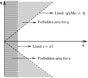
We thus have to find a framework in a subset of the plane (e,q)𝑒𝑞(e,q) such that the limits are better behaved. A natural choice presented above is the line q=0𝑞0q=0 but it is too restrictive. In order to naturally introduce the relevant subset of ΩΩ\Omega, let us consider the other example with ρ1=αxβsubscript𝜌1𝛼superscript𝑥𝛽\rho_{1}=\alpha x^{\beta}, ρ2=1subscript𝜌21\rho_{2}=1, v1=γxδsubscript𝑣1𝛾superscript𝑥𝛿v_{1}=\gamma x^{\delta} and v2=0subscript𝑣20v_{2}=0, with α>0𝛼0\alpha>0, γ>0𝛾0\gamma>0, β0𝛽0\beta\geq 0 and δ0𝛿0\delta\geq 0. As x𝑥x approaches zero, the moment vector 𝐌=(1+αxβ,αγxβ+δ,αγ2xβ+2δ,αγ3xβ+3δ)t𝐌superscript1𝛼superscript𝑥𝛽𝛼𝛾superscript𝑥𝛽𝛿𝛼superscript𝛾2superscript𝑥𝛽2𝛿𝛼superscript𝛾3superscript𝑥𝛽3𝛿𝑡{\bf M}=(1+\alpha x^{\beta},\alpha\gamma x^{\beta+\delta},\alpha\gamma^{2}x^{\beta+2\delta},\alpha\gamma^{3}x^{\beta+3\delta})^{t} reaches the frontier ΓΓ\Gamma of the moment space222The corresponding values of e𝑒e and q𝑞q are e=αγ2xβ+2δ𝑒𝛼superscript𝛾2superscript𝑥𝛽2𝛿e=\alpha\gamma^{2}x^{\beta+2\delta} and q=αγ3xβ+3δ(1αxβ)𝑞𝛼superscript𝛾3superscript𝑥𝛽3𝛿1𝛼superscript𝑥𝛽q=\alpha\gamma^{3}x^{\beta+3\delta}(1-\alpha x^{\beta}).. Two cases are interesting; firstly when β=0𝛽0\beta=0, we reach the point (0,0)00(0,0) in the (e,q)𝑒𝑞(e,q) plane asymptotically along the line q/e3/2=(1α)/α1/2𝑞superscript𝑒321𝛼superscript𝛼12q/e^{3/2}=(1-\alpha)/\alpha^{1/2} and no weight is approaching zero, whereas the two abscissas are joining (see formulas in the proof above). Secondly, when δ=0𝛿0\delta=0, one of the weights is reaching zero, whereas the two abscissas remain different at a distance of γ𝛾\gamma at the limit and we reach the point (0,0)00(0,0) in the (e,q)𝑒𝑞(e,q) plane asymptotically along the line q/(M0e)=γ𝑞subscript𝑀0𝑒𝛾q/(M_{0}\,e)=\gamma at the limit x0𝑥0x\to 0 (see again formulas in the proof above). We will prove in the following proposition that the proper framework is a symmetric cone in the (e,q)𝑒𝑞(e,q) plane centered at the point (0,0)00(0,0) corresponding the |q/(M0e)|η𝑞subscript𝑀0𝑒𝜂|q/(M_{0}\,e)|\leq\eta, where η𝜂\eta is a measure of the maximal distance allowed between the two abscissas.

Definition 2.6 (Regular path).

We define a regular path parametrized by x𝑥x in the moment space, 𝐌x=(M0x,M1x,M2xM3x)subscript𝐌𝑥subscript𝑀0𝑥subscript𝑀1𝑥subscript𝑀2𝑥subscript𝑀3𝑥{\bf M}_{x}=(M_{0\,x},M_{1\,x},M_{2\,x}M_{3\,x}) which admits a limit as x𝑥x goes to zero and is at least 𝒞1superscript𝒞1{\mathcal{C}}^{1} up to the limit 𝐌0subscript𝐌0{\bf M}_{0}. Moreover, we define its reduced second and third order moments ex=M0xM2xM1x2subscript𝑒𝑥subscript𝑀0𝑥subscript𝑀2𝑥superscriptsubscript𝑀1𝑥2e_{x}=M_{0\,x}M_{2\,x}-M_{1\,x}^{2} and qx=(M3xM0xM1x3)3M1x(M0xM2xM1x2)subscript𝑞𝑥subscript𝑀3𝑥subscript𝑀0𝑥superscriptsubscript𝑀1𝑥33subscript𝑀1𝑥subscript𝑀0𝑥subscript𝑀2𝑥superscriptsubscript𝑀1𝑥2q_{x}=(M_{3\,x}M_{0\,x}-M_{1\,x}^{3})-3M_{1\,x}(M_{0\,x}M_{2\,x}-M_{1\,x}^{2}). Its limit further satisfies e0=ex=0=0subscript𝑒0subscript𝑒𝑥00e_{0}=e_{x=0}=0 and we assume ex>0>0subscript𝑒𝑥00e_{x>0}>0, M0x>ν>0subscript𝑀0𝑥𝜈0M_{0\,x}>\nu>0, |qx/(M0xex)|ηsubscript𝑞𝑥subscript𝑀0𝑥subscript𝑒𝑥𝜂|q_{x}/(M_{0\,x}\,e_{x})|\leq\eta, where η>0𝜂0\eta>0.

Proposition 2.7.

We then have the following properties :

  • limx0qx=q0=0subscript𝑥0subscript𝑞𝑥subscript𝑞00\lim_{x\to 0}q_{x}=q_{0}=0.

  • the weights and abscissas admit limits ρi 0=limx0ρixsubscript𝜌𝑖 0subscript𝑥0subscript𝜌𝑖𝑥\rho_{i\,0}=\lim_{x\to 0}\rho_{i\,x}, vi 0=limx0vixsubscript𝑣𝑖 0subscript𝑥0subscript𝑣𝑖𝑥v_{i\,0}=\lim_{x\to 0}v_{i\,x}. If we assume that ρi 0>0subscript𝜌𝑖 00\rho_{i\,0}>0 for both i𝑖i, then v1 0=v2 0subscript𝑣10subscript𝑣20v_{1\,0}=v_{2\,0}, or, if one weight approaches zero, such as ρ1 0=0subscript𝜌100\rho_{1\,0}=0 then we have |v1 0v2 0|ηsubscript𝑣10subscript𝑣20𝜂|v_{1\,0}-v_{2\,0}|\leq\eta and η𝜂\eta is then a bound on the distance between the two abscissas.

  • 𝐌0=(M0 0,M1 0,M1 02/M0 0,M1 03/M0 02)tsubscript𝐌0superscriptsubscript𝑀00subscript𝑀10superscriptsubscript𝑀102subscript𝑀00superscriptsubscript𝑀103superscriptsubscript𝑀002𝑡{\bf M}_{0}=(M_{0\,0},M_{1\,0},M_{1\,0}^{2}/M_{0\,0},M_{1\,0}^{3}/M_{0\,0}^{2})^{t}.

Proof 2.8.

It is first clear that limx0qx=q0=0subscript𝑥0subscript𝑞𝑥subscript𝑞00\lim_{x\to 0}q_{x}=q_{0}=0 since |qx|ηM0xexsubscript𝑞𝑥𝜂subscript𝑀0𝑥subscript𝑒𝑥|q_{x}|\leq\eta M_{0\,x}\,e_{x} and e0=0subscript𝑒00e_{0}=0. Then, easy calculations give

v1v2=q2M02e2+4eM02subscript𝑣1subscript𝑣2superscript𝑞2superscriptsubscript𝑀02superscript𝑒24𝑒superscriptsubscript𝑀02v_{1}-v_{2}=\sqrt{\frac{q^{2}}{M_{0}^{2}e^{2}}+\frac{4e}{M_{0}^{2}}}\\

so that denoting l=limx0|qx|/(M0xex)0𝑙subscript𝑥0subscript𝑞𝑥subscript𝑀0𝑥subscript𝑒𝑥0l=\lim_{x\to 0}|q_{x}|/(M_{0x}e_{x})\geq 0, we clearly have v1xv2xlsubscript𝑣1𝑥subscript𝑣2𝑥𝑙v_{1x}-v_{2x}\to l when x0𝑥0x\to 0 and η𝜂\eta represents an upper bound for v1 0v2 0subscript𝑣10subscript𝑣20v_{1\,0}-v_{2\,0}. Let us now distinguish between the cases l>0𝑙0l>0 and l=0𝑙0l=0. We first note the following expression for q/(M0e)𝑞subscript𝑀0𝑒q/(M_{0}\,e) :

qM0e=(ω1ω2)(v2v1),ωi=ρi/M0,ω1+ω2=1.formulae-sequence𝑞subscript𝑀0𝑒subscript𝜔1subscript𝜔2subscript𝑣2subscript𝑣1formulae-sequencesubscript𝜔𝑖subscript𝜌𝑖subscript𝑀0subscript𝜔1subscript𝜔21\frac{q}{M_{0}\,e}=(\omega_{1}-\omega_{2})(v_{2}-v_{1}),\quad\omega_{i}=\rho_{i}/M_{0},\quad\omega_{1}+\omega_{2}=1.

If l>0𝑙0l>0, one can write

|ρ1xρ2x|=|qxM0xex|×1|v1xv2x|×M0x,subscript𝜌1𝑥subscript𝜌2𝑥subscript𝑞𝑥subscript𝑀0𝑥subscript𝑒𝑥1subscript𝑣1𝑥subscript𝑣2𝑥subscript𝑀0𝑥|\rho_{1\,x}-\rho_{2\,x}|=|\frac{q_{x}}{M_{0\,x}\,e_{x}}|\times\frac{1}{|v_{1\,x}-v_{2\,x}|}\times M_{0\,x},

and this quantity clearly tends to M0 0subscript𝑀00M_{0\,0} as x𝑥x goes to zero. Which means that one weight approaches zero, ρ1 0=0subscript𝜌100\rho_{1\,0}=0 or ρ2 0=0subscript𝜌200\rho_{2\,0}=0, and the other one M0 0subscript𝑀00M_{0\,0} (with ρ1x+ρ2x=M0xsubscript𝜌1𝑥subscript𝜌2𝑥subscript𝑀0𝑥\rho_{1\,x}+\rho_{2\,x}=M_{0\,x}).
If l=0𝑙0l=0, it is clear by the following formula for v1subscript𝑣1v_{1} (see the proof above)

v1=M1M0+q+q2+4e32M0esubscript𝑣1subscript𝑀1subscript𝑀0𝑞superscript𝑞24superscript𝑒32subscript𝑀0𝑒v_{1}=\frac{M_{1}}{M_{0}}+\frac{q+\sqrt{q^{2}+4e^{3}}}{2M_{0}e}

that v1 0=v2 0=M1 0/M0 0subscript𝑣10subscript𝑣20subscript𝑀10subscript𝑀00v_{1\,0}=v_{2\,0}=M_{1\,0}/M_{0\,0}. Using now the definition of ρ1subscript𝜌1\rho_{1} and ρ2subscript𝜌2\rho_{2} (see again the proof above), one easily get

ω2=ρ2M0=1+4e3/q2+sign(q)21+4e3/q2,ω1=ρ1M0=1+4e3/q2sign(q)21+4e3/q2,formulae-sequencesubscript𝜔2subscript𝜌2subscript𝑀014superscript𝑒3superscript𝑞2𝑠𝑖𝑔𝑛𝑞214superscript𝑒3superscript𝑞2subscript𝜔1subscript𝜌1subscript𝑀014superscript𝑒3superscript𝑞2𝑠𝑖𝑔𝑛𝑞214superscript𝑒3superscript𝑞2\omega_{2}=\frac{\rho_{2}}{M_{0}}=\frac{\sqrt{1+4e^{3}/q^{2}}+sign(q)}{2\sqrt{1+4e^{3}/q^{2}}},\quad\omega_{1}=\frac{\rho_{1}}{M_{0}}=\frac{\sqrt{1+4e^{3}/q^{2}}-sign(q)}{2\sqrt{1+4e^{3}/q^{2}}},

so that both weights have limits depending on the limit of q/e3/2𝑞superscript𝑒32q/e^{3/2}.
Clearly, 𝐌0=(M0 0,M1 0,M1 02/M0 0,M1 03/M0 02)tsubscript𝐌0superscriptsubscript𝑀00subscript𝑀10superscriptsubscript𝑀102subscript𝑀00superscriptsubscript𝑀103superscriptsubscript𝑀002𝑡{\bf M}_{0}=(M_{0\,0},M_{1\,0},M_{1\,0}^{2}/M_{0\,0},M_{1\,0}^{3}/M_{0\,0}^{2})^{t}, which completes the proof.

A very important consequence of the previous proposition is the fact that along smooth paths inside the proposed cone which reach the point (0,0)00(0,0) in the (e,q)𝑒𝑞(e,q) plane, the flux introduced in equation 2.3 is regular up to the frontier of the moment space, even if the mapping of 𝐌𝐌{\bf M} onto 𝐔𝐔{\bf U} is not333The mapping of 𝐌𝐌{\bf M} onto 𝐔𝐔{\bf U} will never be smooth at point (0,0)00(0,0) in the (e,q)𝑒𝑞(e,q) plane since the limit of 𝐔𝐔{\bf U} will depend on the limit of q/(M0e)𝑞subscript𝑀0𝑒q/(M_{0}e), whereas the limit value of 𝐌𝐌{\bf M} in the proposed cone is always fixed.

Proposition 2.9.

For any regular path in the moment space satisfying the assumptions of the previous proposition, that is living in the proper cone in the (e,q)𝑒𝑞(e,q) plane and reaching smoothly the point (0,0)00(0,0), the flux 𝐅(𝐌)𝐅𝐌{\bf F}({\bf M}) is continuous up to the frontier of the moment space and 𝒞1superscript𝒞1{\mathcal{C}}^{1} at (0,0)00(0,0) in any direction inside the proposed cone.

Proof 2.10.

The proof is rather straightforward when one has noticed the two equations, the first of which is the expression (2.8) of M4¯=σ0M2σ1M3¯subscript𝑀4subscript𝜎0subscript𝑀2subscript𝜎1subscript𝑀3\overline{M_{4}}=-\sigma_{0}\,M_{2}-\sigma_{1}\,M_{3} as a function of M2subscript𝑀2M_{2}, M3subscript𝑀3M_{3}, σ0subscript𝜎0\sigma_{0} and σ1subscript𝜎1\sigma_{1}, and the second is the expression of σ0subscript𝜎0\sigma_{0} and σ1subscript𝜎1\sigma_{1} :

(σ0σ1)=(qM0eM1M0+(M1M0)2eM02qM0e2M1M0).subscript𝜎0subscript𝜎1𝑞subscript𝑀0𝑒subscript𝑀1subscript𝑀0superscriptsubscript𝑀1subscript𝑀02𝑒superscriptsubscript𝑀02𝑞subscript𝑀0𝑒2subscript𝑀1subscript𝑀0\left(\begin{array}[]{c}\sigma_{0}\vphantom{\displaystyle\frac{q}{M_{0}\,e}}\\ \sigma_{1}\vphantom{\Biggl{(}}\\ \end{array}\right)=\left(\begin{array}[]{c}\displaystyle\frac{q}{M_{0}\,e}\frac{M_{1}}{M_{0}}+\left(\frac{M_{1}}{M_{0}}\right)^{2}-\frac{e}{M_{0}^{2}}\\ \displaystyle-\frac{q}{M_{0}\,e}-2\,\frac{M_{1}}{M_{0}}\vphantom{\Biggl{(}}\end{array}\right).

Finally, following the same lines for the evaluation of the Jacobian matrix of the flux (see matrix J𝐽J in section 2.2), it becomes clear that the flux is continuous and continuously differentiable in any direction inside the proposed cone. Besides, it can be easily seen that the expression of the flux as a function of (M0,M1,e,q)tsuperscriptsubscript𝑀0subscript𝑀1𝑒𝑞𝑡(M_{0},M_{1},e,q)^{t} becomes

M4¯M0=(qM0eM1M0+(M1M0)2eM02)(eM02+(M1M0)2)+(qM0e+2M1M0)(qM03+(M1M0)3+3M1M0eM02).¯subscript𝑀4subscript𝑀0𝑞subscript𝑀0𝑒subscript𝑀1subscript𝑀0superscriptsubscript𝑀1subscript𝑀02𝑒superscriptsubscript𝑀02𝑒superscriptsubscript𝑀02superscriptsubscript𝑀1subscript𝑀02𝑞subscript𝑀0𝑒2subscript𝑀1subscript𝑀0𝑞superscriptsubscript𝑀03superscriptsubscript𝑀1subscript𝑀033subscript𝑀1subscript𝑀0𝑒superscriptsubscript𝑀02\begin{split}\frac{\overline{M_{4}}}{M_{0}}=-\left(\frac{q}{M_{0}\,e}\,\frac{M_{1}}{M_{0}}+\left(\frac{M_{1}}{M_{0}}\right)^{2}-\frac{e}{M_{0}^{2}}\right)\left(\frac{e}{M_{0}^{2}}+\left(\frac{M_{1}}{M_{0}}\right)^{2}\right)+\\ \left(\frac{q}{M_{0}\,e}+2\,\frac{M_{1}}{M_{0}}\right)\left(\frac{q}{M_{0}^{3}}+\left(\frac{M_{1}}{M_{0}}\right)^{3}+3\frac{M_{1}}{M_{0}}\,\frac{e}{M_{0}^{2}}\right).\end{split}

M4¯/M0¯subscript𝑀4subscript𝑀0\overline{M_{4}}/M_{0} tends to (M10/M00)4superscriptsubscript𝑀10subscript𝑀004(M_{10}/M_{00})^{4} when e𝑒e goes to 0+superscript00^{+} which concludes the proof.

Remark 1.

Let us emphasize that in the various configurations we have proposed when the convergence toward the frontier of the moment space does not lie inside the cone |qx/(M0xex)|ηsubscript𝑞𝑥subscript𝑀0𝑥subscript𝑒𝑥𝜂|q_{x}/(M_{0\,x}\,e_{x})|\leq\eta in the (e,q)𝑒𝑞(e,q) plane, the flux can dramatically loose regularity. It can either have a limit without being differentiable or even not have a limit at all. The impact of the previous proposition thus becomes clear and sets the proper framework for solutions which will reach the frontier of the moment space.

Remark 2.

In the case M0>0subscript𝑀00M_{0}>0, at the frontier of the moment space within the previous proposed framework, we have e=0𝑒0e=0, q=0𝑞0q=0; the model is made of the two unknowns M0subscript𝑀0M_{0} and M1subscript𝑀1M_{1} and then degenerates to the usual pressureless gas dynamics which is weakly hyperbolic with a single eigenvalue v=M1/M0𝑣subscript𝑀1subscript𝑀0v=M_{1}/M_{0}. It should be noticed that for smooth solutions, the last two equations of system 2.2 on M2=M12/M0subscript𝑀2superscriptsubscript𝑀12subscript𝑀0M_{2}=M_{1}^{2}/M_{0} and M3=M13/M02subscript𝑀3superscriptsubscript𝑀13superscriptsubscript𝑀02M_{3}=M_{1}^{3}/M_{0}^{2} are still satisfied with M4¯=M14/M03¯subscript𝑀4superscriptsubscript𝑀14superscriptsubscript𝑀03\overline{M_{4}}=M_{1}^{4}/M_{0}^{3} coherent with the previous limit obtained for the flux. As a consequence, we can notice, that at least for smooth solutions, the system of partial differential equations (2.2) can describe the dynamics inside and at the frontier of the moment space.

3 Entropy conditions

In this section, we will work in the interior of the moment space and we exhibit natural entropy inequalities for the following small viscosity system associated with (2.2) :

{tM0+xM1=εxxM0,tM1+xM2=εxxM1,tM2+xM3=εxxM2,tM3+xM4=εxxM3,casessubscript𝑡subscript𝑀0subscript𝑥subscript𝑀1𝜀subscript𝑥𝑥subscript𝑀0subscript𝑡subscript𝑀1subscript𝑥subscript𝑀2𝜀subscript𝑥𝑥subscript𝑀1subscript𝑡subscript𝑀2subscript𝑥subscript𝑀3𝜀subscript𝑥𝑥subscript𝑀2subscript𝑡subscript𝑀3subscript𝑥subscript𝑀4𝜀subscript𝑥𝑥subscript𝑀3\left\{\begin{array}[]{l}\partial_{t}M_{0}+\partial_{x}M_{1}=\varepsilon\partial_{xx}M_{0},\\ \partial_{t}M_{1}+\partial_{x}M_{2}=\varepsilon\partial_{xx}M_{1},\\ \partial_{t}M_{2}+\partial_{x}M_{3}=\varepsilon\partial_{xx}M_{2},\\ \partial_{t}M_{3}+\partial_{x}M_{4}=\varepsilon\partial_{xx}M_{3},\end{array}\right. (3.9)

which gives in condensed form

t𝐌+x𝐅(𝐌)=εxx𝐌.subscript𝑡𝐌subscript𝑥𝐅𝐌𝜀subscript𝑥𝑥𝐌\partial_{t}{\bf M}+\partial_{x}{\bf F}({\bf M})=\varepsilon\partial_{xx}{\bf M}. (3.10)

Throughout this section, we will consider smooth solutions only. We thus have

t𝐌+𝐉x𝐌=εxx𝐌with𝐉=𝐌𝐅.formulae-sequencesubscript𝑡𝐌𝐉subscript𝑥𝐌𝜀subscript𝑥𝑥𝐌with𝐉subscript𝐌𝐅\partial_{t}{\bf M}+{\bf J}\partial_{x}{\bf M}=\varepsilon\partial_{xx}{\bf M}\quad\mbox{with}\quad{\bf J}=\nabla_{{\bf M}}{\bf F}.

Setting 𝐀=𝐔𝐌𝐀subscript𝐔𝐌{\bf A}=\nabla_{{\bf U}}{\bf M}, we then get

t𝐔+𝐀1𝐉𝐀x𝐔=ε𝐀1x(𝐀x𝐔).subscript𝑡𝐔superscript𝐀1𝐉𝐀subscript𝑥𝐔𝜀superscript𝐀1subscript𝑥𝐀subscript𝑥𝐔\partial_{t}{\bf U}+{\bf A}^{-1}{\bf J}{\bf A}\partial_{x}{\bf U}=\varepsilon{\bf A}^{-1}\partial_{x}({\bf A}\partial_{x}{\bf U}). (3.11)

Our objective is to prove that

tη+xqεxxη,subscript𝑡𝜂subscript𝑥𝑞𝜀subscript𝑥𝑥𝜂\partial_{t}\eta+\partial_{x}q\leq\varepsilon\partial_{xx}\eta, (3.12)

for a natural choice of couple (η,q)𝜂𝑞(\eta,q) given by

{η=ρ1S(v1)+ρ2S(v2),q=ρ1v1S(v1)+ρ2v2S(v2).cases𝜂subscript𝜌1𝑆subscript𝑣1subscript𝜌2𝑆subscript𝑣2𝑞subscript𝜌1subscript𝑣1𝑆subscript𝑣1subscript𝜌2subscript𝑣2𝑆subscript𝑣2\left\{\begin{array}[]{l}\eta=\rho_{1}S(v_{1})+\rho_{2}S(v_{2}),\\ q=\rho_{1}v_{1}S(v_{1})+\rho_{2}v_{2}S(v_{2}).\end{array}\right. (3.13)

Here S𝑆S denotes a convex function from \mathbb{R} to \mathbb{R}, and we will especially consider the case where S(v)=v2α𝑆𝑣superscript𝑣2𝛼S(v)=v^{2\alpha}, α0𝛼0\alpha\geq 0. Of course, the densities ρ1subscript𝜌1\rho_{1}, ρ2subscript𝜌2\rho_{2} and velocities v1subscript𝑣1v_{1}, v2subscript𝑣2v_{2} involved in (3.13) are naturally defined by means of the one-to-one and onto function 𝐔=𝐔(𝐌)𝐔𝐔𝐌{\bf U}={\bf U}({\bf M}). In the following and with a little abuse in the notations, we will consider without distinction η𝜂\eta and q𝑞q as functions of 𝐌𝐌{\bf M} or 𝐔𝐔{\bf U}.
 
We first observe

tη+xq=tη(𝐔)+xq(𝐔)=𝐔ηt𝐔+𝐔qx𝐔=𝐔η{𝐀1𝐉𝐀x𝐔+ε𝐀1x(𝐀x𝐔)}+𝐔qx𝐔.subscript𝑡𝜂subscript𝑥𝑞subscript𝑡𝜂𝐔subscript𝑥𝑞𝐔missing-subexpressionsubscript𝐔𝜂subscript𝑡𝐔subscript𝐔𝑞subscript𝑥𝐔missing-subexpressionsubscript𝐔𝜂superscript𝐀1𝐉𝐀subscript𝑥𝐔𝜀superscript𝐀1subscript𝑥𝐀subscript𝑥𝐔subscript𝐔𝑞subscript𝑥𝐔\begin{array}[]{rcl}\partial_{t}\eta+\partial_{x}q&=&\partial_{t}\eta({\bf U})+\partial_{x}q({\bf U})\\ &=&\nabla_{{\bf U}}\eta\partial_{t}{\bf U}+\nabla_{{\bf U}}q\partial_{x}{\bf U}\\ &=&\nabla_{{\bf U}}\eta\{-{\bf A}^{-1}{\bf J}{\bf A}\partial_{x}{\bf U}+\varepsilon{\bf A}^{-1}\partial_{x}({\bf A}\partial_{x}{\bf U})\}+\nabla_{{\bf U}}q\partial_{x}{\bf U}.\end{array}

The following two lemmas, the proofs of which are left to the reader, will be useful in order to estimate the entropy dissipation rate 𝐃𝐃{\bf D} defined by

𝐃=𝐔η{𝐀1𝐉𝐀x𝐔+ε𝐀1x(𝐀x𝐔)}+𝐔qx𝐔.𝐃subscript𝐔𝜂superscript𝐀1𝐉𝐀subscript𝑥𝐔𝜀superscript𝐀1subscript𝑥𝐀subscript𝑥𝐔subscript𝐔𝑞subscript𝑥𝐔{\bf D}=\nabla_{{\bf U}}\eta\{-{\bf A}^{-1}{\bf J}{\bf A}\partial_{x}{\bf U}+\varepsilon{\bf A}^{-1}\partial_{x}({\bf A}\partial_{x}{\bf U})\}+\nabla_{{\bf U}}q\partial_{x}{\bf U}.
Lemma 3.1.

The matrices 𝐉𝐉{\bf J} and 𝐀𝐀{\bf A} and 𝐀1𝐉𝐀superscript𝐀1𝐉𝐀{\bf A}^{-1}{\bf J}{\bf A} are given by

𝐉=(010000100001v12v222v1v2(v1+v2)2v1v2(v1+v2)22(v1+v2)),𝐉010000100001superscriptsubscript𝑣12superscriptsubscript𝑣222subscript𝑣1subscript𝑣2subscript𝑣1subscript𝑣22subscript𝑣1subscript𝑣2superscriptsubscript𝑣1subscript𝑣222subscript𝑣1subscript𝑣2{\bf J}=\left(\begin{array}[]{cccc}0&1&0&0\\ 0&0&1&0\\ 0&0&0&1\\ -v_{1}^{2}v_{2}^{2}&2v_{1}v_{2}(v_{1}+v_{2})&-2v_{1}v_{2}-(v_{1}+v_{2})^{2}&2(v_{1}+v_{2})\\ \end{array}\right),
𝐀=(11000011v12v222v12v22v132v233v123v22),𝐀1𝐉𝐀=(00100001v1202v100v2202v2).formulae-sequence𝐀11000011superscriptsubscript𝑣12superscriptsubscript𝑣222subscript𝑣12subscript𝑣22superscriptsubscript𝑣132superscriptsubscript𝑣233superscriptsubscript𝑣123superscriptsubscript𝑣22superscript𝐀1𝐉𝐀00100001superscriptsubscript𝑣1202subscript𝑣100superscriptsubscript𝑣2202subscript𝑣2{\bf A}=\left(\begin{array}[]{cccc}1&1&0&0\\ 0&0&1&1\\ -v_{1}^{2}&-v_{2}^{2}&2v_{1}&2v_{2}\\ -2v_{1}^{3}&-2v_{2}^{3}&3v_{1}^{2}&3v_{2}^{2}\\ \end{array}\right),\quad{\bf A}^{-1}{\bf J}{\bf A}=\left(\begin{array}[]{cccc}0&0&1&0\\ 0&0&0&1\\ -v_{1}^{2}&0&2v_{1}&0\\ 0&-v_{2}^{2}&0&2v_{2}\\ \end{array}\right).
Lemma 3.2.

The gradients 𝐔ηsubscript𝐔𝜂\nabla_{{\bf U}}\eta and 𝐔qsubscript𝐔𝑞\nabla_{{\bf U}}q are given by

𝐔η=(S(v1)v1S(v1)S(v2)v2S(v2)S(v1)S(v2))t,𝐔q=(v12S(v1)v22S(v2)S(v1)+v1S(v1)S(v1)+v1S(v1))t,formulae-sequencesubscript𝐔𝜂superscript𝑆subscript𝑣1subscript𝑣1superscript𝑆subscript𝑣1𝑆subscript𝑣2subscript𝑣2superscript𝑆subscript𝑣2superscript𝑆subscript𝑣1superscript𝑆subscript𝑣2𝑡subscript𝐔𝑞superscriptsuperscriptsubscript𝑣12superscript𝑆subscript𝑣1superscriptsubscript𝑣22superscript𝑆subscript𝑣2𝑆subscript𝑣1subscript𝑣1superscript𝑆subscript𝑣1𝑆subscript𝑣1subscript𝑣1superscript𝑆subscript𝑣1𝑡\nabla_{{\bf U}}\eta=\left(\begin{array}[]{c}S(v_{1})-v_{1}S^{{}^{\prime}}(v_{1})\\ S(v_{2})-v_{2}S^{{}^{\prime}}(v_{2})\\ S^{{}^{\prime}}(v_{1})\\ S^{{}^{\prime}}(v_{2})\\ \end{array}\right)^{t},\quad\nabla_{{\bf U}}q=\left(\begin{array}[]{c}-v_{1}^{2}S^{{}^{\prime}}(v_{1})\\ -v_{2}^{2}S^{{}^{\prime}}(v_{2})\\ S(v_{1})+v_{1}S^{{}^{\prime}}(v_{1})\\ S(v_{1})+v_{1}S^{{}^{\prime}}(v_{1})\\ \end{array}\right)^{t},

and we have

𝐔q=𝐔η𝐀1𝐉𝐀.subscript𝐔𝑞subscript𝐔𝜂superscript𝐀1𝐉𝐀\nabla_{{\bf U}}q=\nabla_{{\bf U}}\eta{\bf A}^{-1}{\bf J}{\bf A}.

Before going on, let us make the following two remarks. We first note that thanks to the first lemma, (3.11) with ε=0𝜀0\varepsilon=0 inside the moment space gives :

{tρ1+xρ1v1=0,tρ2+xρ2v2=0,tρ1v1v12xρ1+2v1xρ1v1=0,tρ2v2v22xρ2+2v2xρ2v2=0,casessubscript𝑡subscript𝜌1subscript𝑥subscript𝜌1subscript𝑣10subscript𝑡subscript𝜌2subscript𝑥subscript𝜌2subscript𝑣20subscript𝑡subscript𝜌1subscript𝑣1superscriptsubscript𝑣12subscript𝑥subscript𝜌12subscript𝑣1subscript𝑥subscript𝜌1subscript𝑣10subscript𝑡subscript𝜌2subscript𝑣2superscriptsubscript𝑣22subscript𝑥subscript𝜌22subscript𝑣2subscript𝑥subscript𝜌2subscript𝑣20\left\{\begin{array}[]{l}\partial_{t}\rho_{1}+\partial_{x}\rho_{1}v_{1}=0,\\ \partial_{t}\rho_{2}+\partial_{x}\rho_{2}v_{2}=0,\\ \partial_{t}\rho_{1}v_{1}-v_{1}^{2}\partial_{x}\rho_{1}+2v_{1}\partial_{x}\rho_{1}v_{1}=0,\\ \partial_{t}\rho_{2}v_{2}-v_{2}^{2}\partial_{x}\rho_{2}+2v_{2}\partial_{x}\rho_{2}v_{2}=0,\\ \end{array}\right.

which is equivalent to

{tρ1+xρ1v1=0,tρ1v1+xρ1v12=0,tρ2+xρ2v2=0,tρ2v2+xρ2v22=0.casessubscript𝑡subscript𝜌1subscript𝑥subscript𝜌1subscript𝑣10subscript𝑡subscript𝜌1subscript𝑣1subscript𝑥subscript𝜌1superscriptsubscript𝑣120subscript𝑡subscript𝜌2subscript𝑥subscript𝜌2subscript𝑣20subscript𝑡subscript𝜌2subscript𝑣2subscript𝑥subscript𝜌2superscriptsubscript𝑣220\left\{\begin{array}[]{l}\partial_{t}\rho_{1}+\partial_{x}\rho_{1}v_{1}=0,\\ \partial_{t}\rho_{1}v_{1}+\partial_{x}\rho_{1}v_{1}^{2}=0,\\ \partial_{t}\rho_{2}+\partial_{x}\rho_{2}v_{2}=0,\\ \partial_{t}\rho_{2}v_{2}+\partial_{x}\rho_{2}v_{2}^{2}=0.\\ \end{array}\right. (3.14)

Besides, at the frontier of the moment space, we obtain the pressureless gas dynamics on a single quadrature node. We then observe that for smooth solutions, thanks to the remark at the end of the previous section, the system (2.3) is nothing but either two decoupled or one single pressureless gas dynamics system of equations. We then observe that still with ε=0𝜀0\varepsilon=0, 𝐃=0𝐃0{\bf D}=0, by lemma 3.2, in both cases :

tη+xq=0,subscript𝑡𝜂subscript𝑥𝑞0\partial_{t}\eta+\partial_{x}q=0, (3.15)

that is for smooth solution both inside and at the frontier of the moment space.

Let us go back to the case ε>0𝜀0\varepsilon>0. We thus have the following equality,

𝐃=ε𝐔η𝐀1x(𝐀x𝐔),𝐃𝜀subscript𝐔𝜂superscript𝐀1subscript𝑥𝐀subscript𝑥𝐔{\bf D}=\varepsilon\nabla_{{\bf U}}\eta{\bf A}^{-1}\partial_{x}({\bf A}\partial_{x}{\bf U}),

from which it is natural to isolate εxxη𝜀subscript𝑥𝑥𝜂\varepsilon\partial_{xx}\eta :

𝐃=ε𝐔η𝐀1x(𝐀x𝐔)=ε𝐔ηxx𝐔+ε𝐔η𝐀1x𝐀x𝐔=εx(𝐔ηx𝐔)εx(𝐔η)x𝐔+ε𝐔η𝐀1x𝐀x𝐔=εxxη+ε(𝐔η𝐀1x𝐀x𝐔x(𝐔η)x𝐔).𝐃𝜀subscript𝐔𝜂superscript𝐀1subscript𝑥𝐀subscript𝑥𝐔missing-subexpression𝜀subscript𝐔𝜂subscript𝑥𝑥𝐔𝜀subscript𝐔𝜂superscript𝐀1subscript𝑥𝐀subscript𝑥𝐔missing-subexpression𝜀subscript𝑥subscript𝐔𝜂subscript𝑥𝐔𝜀subscript𝑥subscript𝐔𝜂subscript𝑥𝐔𝜀subscript𝐔𝜂superscript𝐀1subscript𝑥𝐀subscript𝑥𝐔missing-subexpression𝜀subscript𝑥𝑥𝜂𝜀subscript𝐔𝜂superscript𝐀1subscript𝑥𝐀subscript𝑥𝐔subscript𝑥subscript𝐔𝜂subscript𝑥𝐔\begin{array}[]{rcl}{\bf D}&=&\varepsilon\nabla_{{\bf U}}\eta{\bf A}^{-1}\partial_{x}({\bf A}\partial_{x}{\bf U})\\ &=&\varepsilon\nabla_{{\bf U}}\eta\partial_{xx}{\bf U}+\varepsilon\nabla_{{\bf U}}\eta{\bf A}^{-1}\partial_{x}{\bf A}\partial_{x}{\bf U}\\ &=&\varepsilon\partial_{x}(\nabla_{{\bf U}}\eta\partial_{x}{\bf U})-\varepsilon\partial_{x}(\nabla_{{\bf U}}\eta)\partial_{x}{\bf U}+\varepsilon\nabla_{{\bf U}}\eta{\bf A}^{-1}\partial_{x}{\bf A}\partial_{x}{\bf U}\\ &=&\varepsilon\partial_{xx}\eta+\varepsilon\big{(}\nabla_{{\bf U}}\eta{\bf A}^{-1}\partial_{x}{\bf A}\partial_{x}{\bf U}-\partial_{x}(\nabla_{{\bf U}}\eta)\partial_{x}{\bf U}\big{)}.\\ \end{array}

By lemma 3.2 giving 𝐔ηsubscript𝐔𝜂\nabla_{{\bf U}}\eta, we easily get

x(𝐔η)x𝐔=ρ1(xv1)2S′′(v1)+ρ2(xv2)2S′′(v2).subscript𝑥subscript𝐔𝜂subscript𝑥𝐔subscript𝜌1superscriptsubscript𝑥subscript𝑣12superscript𝑆′′subscript𝑣1subscript𝜌2superscriptsubscript𝑥subscript𝑣22superscript𝑆′′subscript𝑣2\partial_{x}(\nabla_{{\bf U}}\eta)\partial_{x}{\bf U}=\rho_{1}(\partial_{x}v_{1})^{2}S^{{}^{\prime\prime}}(v_{1})+\rho_{2}(\partial_{x}v_{2})^{2}S^{{}^{\prime\prime}}(v_{2}).

It is now a matter to calculate 𝐔η𝐀1x𝐀x𝐔=𝐀t(𝐔η)tx𝐀x𝐔subscript𝐔𝜂superscript𝐀1subscript𝑥𝐀subscript𝑥𝐔superscript𝐀𝑡superscriptsubscript𝐔𝜂𝑡subscript𝑥𝐀subscript𝑥𝐔\nabla_{{\bf U}}\eta{\bf A}^{-1}\partial_{x}{\bf A}\partial_{x}{\bf U}={\bf A}^{-t}(\nabla_{{\bf U}}\eta)^{t}\partial_{x}{\bf A}\partial_{x}{\bf U}. We first observe that

x𝐀x𝐔=(002ρ1(xv1)2+2ρ2(xv2)26ρ1v1(xv1)2+6ρ2v2(xv2)2)subscript𝑥𝐀subscript𝑥𝐔002subscript𝜌1superscriptsubscript𝑥subscript𝑣122subscript𝜌2superscriptsubscript𝑥subscript𝑣226subscript𝜌1subscript𝑣1superscriptsubscript𝑥subscript𝑣126subscript𝜌2subscript𝑣2superscriptsubscript𝑥subscript𝑣22\partial_{x}{\bf A}\partial_{x}{\bf U}=\left(\begin{array}[]{c}0\\ 0\\ 2\rho_{1}(\partial_{x}v_{1})^{2}+2\rho_{2}(\partial_{x}v_{2})^{2}\\ 6\rho_{1}v_{1}(\partial_{x}v_{1})^{2}+6\rho_{2}v_{2}(\partial_{x}v_{2})^{2}\end{array}\right)

so that only the last two components of 𝐀t(𝐔η)tsuperscript𝐀𝑡superscriptsubscript𝐔𝜂𝑡{\bf A}^{-t}(\nabla_{{\bf U}}\eta)^{t} are actually needed. Finally, easy calculations not reported here lead to

𝐀t(𝐔η)tx𝐀x𝐔=1(v1v2)4(2ρ1(xv1)2X1+2ρ2(xv2)2X2),superscript𝐀𝑡superscriptsubscript𝐔𝜂𝑡subscript𝑥𝐀subscript𝑥𝐔1superscriptsubscript𝑣1subscript𝑣242subscript𝜌1superscriptsubscript𝑥subscript𝑣12subscript𝑋12subscript𝜌2superscriptsubscript𝑥subscript𝑣22subscript𝑋2{\bf A}^{-t}(\nabla_{{\bf U}}\eta)^{t}\partial_{x}{\bf A}\partial_{x}{\bf U}=-\frac{1}{(v_{1}-v_{2})^{4}}(2\rho_{1}(\partial_{x}v_{1})^{2}X_{1}+2\rho_{2}(\partial_{x}v_{2})^{2}X_{2}),

where we have set

{X1=(v1v2)2(3(S(v1)S(v2))2(v1v2)S(v1)(v1v2)S(v2)),X2=(v1v2)2(3(S(v1)S(v2))(v1v2)S(v1)2(v1v2)S(v2)).casessubscript𝑋1superscriptsubscript𝑣1subscript𝑣223𝑆subscript𝑣1𝑆subscript𝑣22subscript𝑣1subscript𝑣2superscript𝑆subscript𝑣1subscript𝑣1subscript𝑣2superscript𝑆subscript𝑣2subscript𝑋2superscriptsubscript𝑣1subscript𝑣223𝑆subscript𝑣1𝑆subscript𝑣2subscript𝑣1subscript𝑣2superscript𝑆subscript𝑣12subscript𝑣1subscript𝑣2superscript𝑆subscript𝑣2\left\{\begin{array}[]{l}X_{1}=(v_{1}-v_{2})^{2}\Big{(}3\big{(}S(v_{1})-S(v_{2})\big{)}-2(v_{1}-v_{2})S^{{}^{\prime}}(v_{1})-(v_{1}-v_{2})S^{{}^{\prime}}(v_{2})\Big{)},\\ X_{2}=-(v_{1}-v_{2})^{2}\Big{(}3\big{(}S(v_{1})-S(v_{2})\big{)}-(v_{1}-v_{2})S^{{}^{\prime}}(v_{1})-2(v_{1}-v_{2})S^{{}^{\prime}}(v_{2})\Big{)}.\end{array}\right.

The entropy inequality (3.12) is then valid if and only if

𝐔η𝐀1x𝐀x𝐔x(𝐔η)x𝐔0,subscript𝐔𝜂superscript𝐀1subscript𝑥𝐀subscript𝑥𝐔subscript𝑥subscript𝐔𝜂subscript𝑥𝐔0\nabla_{{\bf U}}\eta{\bf A}^{-1}\partial_{x}{\bf A}\partial_{x}{\bf U}-\partial_{x}(\nabla_{{\bf U}}\eta)\partial_{x}{\bf U}\leq 0,

that is, setting Si=S(vi)subscript𝑆𝑖𝑆subscript𝑣𝑖S_{i}=S(v_{i}), Si=S(vi)subscriptsuperscript𝑆𝑖superscript𝑆subscript𝑣𝑖S^{{}^{\prime}}_{i}=S^{{}^{\prime}}(v_{i}) and Si′′=S′′(vi)subscriptsuperscript𝑆′′𝑖superscript𝑆′′subscript𝑣𝑖S^{{}^{\prime\prime}}_{i}=S^{{}^{\prime\prime}}(v_{i}), i=1,2𝑖12i=1,2,

(v1v2)2ρ1(xv1)2(6(S1S2)4(v1v2)S12(v1v2)S2+(v1v2)2S1′′)+(v1v2)2ρ2(xv2)2(6(S1S2)+2(v1v2)S1+4(v1v2)S2+(v1v2)2S2′′)0.missing-subexpressionsuperscriptsubscript𝑣1subscript𝑣22subscript𝜌1superscriptsubscript𝑥subscript𝑣126subscript𝑆1subscript𝑆24subscript𝑣1subscript𝑣2subscriptsuperscript𝑆12subscript𝑣1subscript𝑣2subscriptsuperscript𝑆2superscriptsubscript𝑣1subscript𝑣22subscriptsuperscript𝑆′′1missing-subexpressionmissing-subexpressionmissing-subexpressionmissing-subexpressionsuperscriptsubscript𝑣1subscript𝑣22subscript𝜌2superscriptsubscript𝑥subscript𝑣226subscript𝑆1subscript𝑆22subscript𝑣1subscript𝑣2subscriptsuperscript𝑆14subscript𝑣1subscript𝑣2subscriptsuperscript𝑆2superscriptsubscript𝑣1subscript𝑣22subscriptsuperscript𝑆′′2missing-subexpressionmissing-subexpressionabsent0absent\begin{array}[]{rcl}&(v_{1}-v_{2})^{2}\rho_{1}(\partial_{x}v_{1})^{2}\Big{(}6\big{(}S_{1}-S_{2}\big{)}-4(v_{1}-v_{2})S^{{}^{\prime}}_{1}-2(v_{1}-v_{2})S^{{}^{\prime}}_{2}+(v_{1}-v_{2})^{2}S^{{}^{\prime\prime}}_{1}\Big{)}&\\ &+&\\ &(v_{1}-v_{2})^{2}\rho_{2}(\partial_{x}v_{2})^{2}\Big{(}-6\big{(}S_{1}-S_{2}\big{)}+2(v_{1}-v_{2})S^{{}^{\prime}}_{1}+4(v_{1}-v_{2})S^{{}^{\prime}}_{2}+(v_{1}-v_{2})^{2}S^{{}^{\prime\prime}}_{2}\Big{)}&\\ &\geq 0&.\end{array} (3.16)

A sufficient condition is given by

{6(S1S2)4(v1v2)S12(v1v2)S2+(v1v2)2S1′′0,6(S1S2)+2(v1v2)S1+4(v1v2)S2+(v1v2)2S2′′0.cases6subscript𝑆1subscript𝑆24subscript𝑣1subscript𝑣2subscriptsuperscript𝑆12subscript𝑣1subscript𝑣2subscriptsuperscript𝑆2superscriptsubscript𝑣1subscript𝑣22subscriptsuperscript𝑆′′106subscript𝑆1subscript𝑆22subscript𝑣1subscript𝑣2subscriptsuperscript𝑆14subscript𝑣1subscript𝑣2subscriptsuperscript𝑆2superscriptsubscript𝑣1subscript𝑣22subscriptsuperscript𝑆′′20\left\{\begin{array}[]{c}6\big{(}S_{1}-S_{2}\big{)}-4(v_{1}-v_{2})S^{{}^{\prime}}_{1}-2(v_{1}-v_{2})S^{{}^{\prime}}_{2}+(v_{1}-v_{2})^{2}S^{{}^{\prime\prime}}_{1}\geq 0,\\ -6\big{(}S_{1}-S_{2}\big{)}+2(v_{1}-v_{2})S^{{}^{\prime}}_{1}+4(v_{1}-v_{2})S^{{}^{\prime}}_{2}+(v_{1}-v_{2})^{2}S^{{}^{\prime\prime}}_{2}\geq 0.\end{array}\right. (3.17)

Let us focus for instance on the first inequality (the second one is treated in a similar way), and let us consider the left-hand side as a function of v2subscript𝑣2v_{2}, for any given v1subscript𝑣1v_{1} :

1(v2)=6(S1S2)4(v1v2)S12(v1v2)S2+(v1v2)2S1′′.subscript1subscript𝑣26subscript𝑆1subscript𝑆24subscript𝑣1subscript𝑣2subscriptsuperscript𝑆12subscript𝑣1subscript𝑣2subscriptsuperscript𝑆2superscriptsubscript𝑣1subscript𝑣22subscriptsuperscript𝑆′′1{\mathcal{F}}_{1}(v_{2})=6(S_{1}-S_{2})-4(v_{1}-v_{2})S^{{}^{\prime}}_{1}-2(v_{1}-v_{2})S^{{}^{\prime}}_{2}+(v_{1}-v_{2})^{2}S^{{}^{\prime\prime}}_{1}.

Differentiation yields

1(v2)=4(S1S2)2(v1v2)(S1′′+S2′′),1′′(v2)=2(S1′′S2′′)2(v1v2)S2′′′,1′′′(v2)=2(v2v1)S2′′′′.superscriptsubscript1subscript𝑣24subscriptsuperscript𝑆1subscriptsuperscript𝑆22subscript𝑣1subscript𝑣2subscriptsuperscript𝑆′′1subscriptsuperscript𝑆′′2superscriptsubscript1′′subscript𝑣22subscriptsuperscript𝑆′′1subscriptsuperscript𝑆′′22subscript𝑣1subscript𝑣2subscriptsuperscript𝑆′′′2superscriptsubscript1′′′subscript𝑣22subscript𝑣2subscript𝑣1subscriptsuperscript𝑆′′′′2\begin{array}[]{l}{\mathcal{F}}_{1}^{{}^{\prime}}(v_{2})=4(S^{{}^{\prime}}_{1}-S^{{}^{\prime}}_{2})-2(v_{1}-v_{2})(S^{{}^{\prime\prime}}_{1}+S^{{}^{\prime\prime}}_{2}),\\ {\mathcal{F}}_{1}^{{}^{\prime\prime}}(v_{2})=2(S^{{}^{\prime\prime}}_{1}-S^{{}^{\prime\prime}}_{2})-2(v_{1}-v_{2})S^{{}^{\prime\prime\prime}}_{2},\\ {\mathcal{F}}_{1}^{{}^{\prime\prime\prime}}(v_{2})=2(v_{2}-v_{1})S^{{}^{\prime\prime\prime\prime}}_{2}.\end{array}

It is then clear that 1(v1)=1(v1)=1′′(v1)=1′′′(v1)=0subscript1subscript𝑣1superscriptsubscript1subscript𝑣1superscriptsubscript1′′subscript𝑣1superscriptsubscript1′′′subscript𝑣10{\mathcal{F}}_{1}(v_{1})={\mathcal{F}}_{1}^{{}^{\prime}}(v_{1})={\mathcal{F}}_{1}^{{}^{\prime\prime}}(v_{1})={\mathcal{F}}_{1}^{{}^{\prime\prime\prime}}(v_{1})=0. Then, provided that S′′′′(v)0superscript𝑆′′′′𝑣0S^{{}^{\prime\prime\prime\prime}}(v)\geq 0, vfor-all𝑣\forall v, we easily get by a chain argument based on the sign of the derivative and the monotonicity property that 1(v2)0subscript1subscript𝑣20{\mathcal{F}}_{1}(v_{2})\geq 0, v1,v2for-allsubscript𝑣1subscript𝑣2\forall v_{1},v_{2}. We have thus proved the following proposition :

Proposition 3.3.

Smooth solutions of (3.10) satisfy the entropy inequality (3.12) for any entropy entropy-flux pair (η,q)𝜂𝑞(\eta,q) defined by (3.13) provided that vS(v)𝑣𝑆𝑣v\to S(v) is a smooth function from \mathbb{R} to \mathbb{R} with nonnegative fourth-order derivative. In particular, the natural choice S(v)=v2α𝑆𝑣superscript𝑣2𝛼S(v)=v^{2\alpha} with α2𝛼2\alpha\geq 2 is suitable.

Remark 1.

Any third-order polynomial may of course be added to the leading term of S𝑆S, without changing the sign of the fourth-order derivative. However, if we focus on (strictly) convex functions vS(v)𝑣𝑆𝑣v\to S(v) in order to get a (strictly) convex entropy η=η(𝐔)𝜂𝜂𝐔\eta=\eta({\bf U}), only first-order polynomials may be added without changing the convexity property.

Remark 2.

If we consider S(v)=1,v,v2,v3𝑆𝑣1𝑣superscript𝑣2superscript𝑣3S(v)=1,v,v^{2},v^{3}, it is easily checked that (3.17) holds true with two equalities. In agreement with (3.9), these choices that lead to the pairs (η,q)=(Mi,Mi+1)𝜂𝑞subscript𝑀𝑖subscript𝑀𝑖1(\eta,q)=(M_{i},M_{i+1}), i=0,,3𝑖03i=0,...,3, are admissible.

Remark 3.

In the case M0>0subscript𝑀00M_{0}>0, e=0𝑒0e=0, q=0𝑞0q=0 with the additional conditions associated with the connection between the interior and the frontier of the moment space presented in subsection 2.3, we clearly have Mk=M1k/M0k1subscript𝑀𝑘superscriptsubscript𝑀1𝑘superscriptsubscript𝑀0𝑘1M_{k}=M_{1}^{k}/M_{0}^{k-1}. In this case, the entropy pairs clearly work also in such a case, for smooth solutions, and admits a smooth behavior at the frontier of the moment space in the cone we have defined previously.

4 Kinetic-macroscopic relation for smooth solutions

For smooth solutions, we established in the previous section that the four-moment model (2.2) is equivalent to the following two decoupled pressureless gas dynamics model

{tρ1+xρ1v1=0,tρ1v1+xρ1v12=0,tρ2+xρ2v2=0,tρ2v2+xρ2v22=0,casessubscript𝑡subscript𝜌1subscript𝑥subscript𝜌1subscript𝑣10subscript𝑡subscript𝜌1subscript𝑣1subscript𝑥subscript𝜌1superscriptsubscript𝑣120subscript𝑡subscript𝜌2subscript𝑥subscript𝜌2subscript𝑣20subscript𝑡subscript𝜌2subscript𝑣2subscript𝑥subscript𝜌2superscriptsubscript𝑣220\left\{\begin{array}[]{l}\partial_{t}\rho_{1}+\partial_{x}\rho_{1}v_{1}=0,\\ \partial_{t}\rho_{1}v_{1}+\partial_{x}\rho_{1}v_{1}^{2}=0,\\ \partial_{t}\rho_{2}+\partial_{x}\rho_{2}v_{2}=0,\\ \partial_{t}\rho_{2}v_{2}+\partial_{x}\rho_{2}v_{2}^{2}=0,\\ \end{array}\right. (4.18)

where ρ1subscript𝜌1\rho_{1}, ρ2subscript𝜌2\rho_{2}, v1subscript𝑣1v_{1} and v2subscript𝑣2v_{2} are defined by the nonlinear system (2.6). The aim of this section is to prove a rigorous equivalence result, still for smooth solutions, between this macroscopic model and the free transport kinetic formulation (2.1) when the velocity distribution is given by a set of two Dirac delta functions. This result is nothing but a generalization of the one given in [Bouchut (1994)] for the usual pressureless gas dynamics model.

Proposition 4.1.

Let T>0𝑇0T>0 and ρi(t,x)subscript𝜌𝑖𝑡𝑥\rho_{i}(t,x), vi(t,x)subscript𝑣𝑖𝑡𝑥v_{i}(t,x) in 𝒞1(]0,T[×)\mathcal{C}^{1}(]0,T[\times\mathbb{R}) for i=1,2𝑖12i=1,2. Let us define

f(t,x,v)=i=12ρi(t,x)δ(vvi(t,x)).𝑓𝑡𝑥𝑣superscriptsubscript𝑖12subscript𝜌𝑖𝑡𝑥𝛿𝑣subscript𝑣𝑖𝑡𝑥f(t,x,v)=\sum_{i=1}^{2}\rho_{i}(t,x)\delta(v-v_{i}(t,x)).

Then, ρisubscript𝜌𝑖\rho_{i} and visubscript𝑣𝑖v_{i} solve (2.2), or equivalently (4.18), in ]0,T[×]0,T[\times\mathbb{R} if and only if

tf+vxf=0,in]0,T[××\partial_{t}f+v\partial_{x}f=0,\quad\mbox{in}\quad]0,T[\times\mathbb{R}\times\mathbb{R} (4.19)

in the distributional sense, i.e. if and only if ϕ𝒞c(]0,T[×)\forall\phi\,\,\in\,\,\mathcal{C}^{\infty}_{c}(]0,T[\times\mathbb{R}) and χ𝒞c()𝜒subscriptsuperscript𝒞𝑐\chi\,\,\in\,\,\mathcal{C}^{\infty}_{c}(\mathbb{R})

0Ti=12ρi(t,x)(tϕ(t,x)+vi(t,x)xϕ(t,x))χ(vi(x,t))=0.superscriptsubscript0𝑇subscriptsuperscriptsubscript𝑖12subscript𝜌𝑖𝑡𝑥subscript𝑡italic-ϕ𝑡𝑥subscript𝑣𝑖𝑡𝑥subscript𝑥italic-ϕ𝑡𝑥𝜒subscript𝑣𝑖𝑥𝑡0\int_{0}^{T}\int_{\mathbb{R}}\sum_{i=1}^{2}\rho_{i}(t,x)\Big{(}\partial_{t}\phi(t,x)+v_{i}(t,x)\partial_{x}\phi(t,x)\Big{)}\chi\big{(}v_{i}(x,t)\big{)}=0.\\ (4.20)
Proof 4.2.

Let us first assume that (4.20) holds true. Since the velocity functions visubscript𝑣𝑖v_{i} are in particular locally bounded, one can successively choose χ𝒞c()𝜒subscriptsuperscript𝒞𝑐\chi\,\,\in\,\,\mathcal{C}^{\infty}_{c}(\mathbb{R}) such that χ(v)=vk𝜒𝑣superscript𝑣𝑘\chi(v)=v^{k}, k=0,,3𝑘03k=0,...,3 for all v=vi(t,x)𝑣subscript𝑣𝑖𝑡𝑥v=v_{i}(t,x) and then get

0Ti=12ρi(t,x)(tϕ(t,x)+vi(t,x)xϕ(t,x))(vi(t,x))k=0superscriptsubscript0𝑇subscriptsuperscriptsubscript𝑖12subscript𝜌𝑖𝑡𝑥subscript𝑡italic-ϕ𝑡𝑥subscript𝑣𝑖𝑡𝑥subscript𝑥italic-ϕ𝑡𝑥superscriptsubscript𝑣𝑖𝑡𝑥𝑘0\int_{0}^{T}\int_{\mathbb{R}}\sum_{i=1}^{2}\rho_{i}(t,x)\Big{(}\partial_{t}\phi(t,x)+v_{i}(t,x)\partial_{x}\phi(t,x)\Big{)}\big{(}v_{i}(t,x)\big{)}^{k}=0

for all ϕ𝒞c(]0,T[×)\phi\,\,\in\,\,\mathcal{C}^{\infty}_{c}(]0,T[\times\mathbb{R}). Invoking the closure relation (2.6), this gives the four-moment model (2.2), or equivalently (4.18), as ρi(t,x)subscript𝜌𝑖𝑡𝑥\rho_{i}(t,x) and vi(t,x)subscript𝑣𝑖𝑡𝑥v_{i}(t,x) are smooth functions.
Conversely, let us assume that the partial differential equations of (4.18) are satisfied. Using the mass conservation equations, it is then usual to show that for i=1,2𝑖12i=1,2

ρi(tvi+vixvi)=0,subscript𝜌𝑖subscript𝑡subscript𝑣𝑖subscript𝑣𝑖subscript𝑥subscript𝑣𝑖0\rho_{i}(\partial_{t}v_{i}+v_{i}\partial_{x}v_{i})=0,

and then multiplying by χsuperscript𝜒\chi^{\prime} for any smooth function χ𝜒\chi,

tρiχ(vi)+xρiχ(vi)vi=0.subscript𝑡subscript𝜌𝑖𝜒subscript𝑣𝑖subscript𝑥subscript𝜌𝑖𝜒subscript𝑣𝑖subscript𝑣𝑖0\partial_{t}\rho_{i}\chi(v_{i})+\partial_{x}\rho_{i}\chi(v_{i})v_{i}=0.

Summing over i=1,2𝑖12i=1,2 and integrating past a test function ϕ𝒞c(]0,T[×)\phi\,\,\in\,\,\mathcal{C}^{\infty}_{c}(]0,T[\times\mathbb{R}) gives the expected result (4.20). This concludes the proof.

This Proposition allows, as a corollary, to introduce a particular type of solution which will be denoted piecewise free boundary 𝒞1superscript𝒞1\mathcal{C}^{1} solutions. Such solutions correspond to a discontinuous connection from the interior of the moment space to the frontier through a contact discontinuity for which the Rankine Hugoniot solutions are trivially satisfied as well as the entropy conservation equation (3.15).

Corollary 4.3.

We consider the following distribution at the kinetic level f(t,x,v)=i=12ρi(t,x)δ(vvi(t,x))𝑓𝑡𝑥𝑣superscriptsubscript𝑖12subscript𝜌𝑖𝑡𝑥𝛿𝑣subscript𝑣𝑖𝑡𝑥f(t,x,v)=\sum_{i=1}^{2}\rho_{i}(t,x)\delta(v-v_{i}(t,x)), where ρ1(t,x)>0subscript𝜌1𝑡𝑥0\rho_{1}(t,x)>0 and v1(t,x)subscript𝑣1𝑡𝑥v_{1}(t,x) are taken as constants (or sufficiently smooth in some time interval), whereas ρ2(t,x)subscript𝜌2𝑡𝑥\rho_{2}(t,x) is zero except in a compact connected subset K0subscript𝐾0K_{0} at time t=0𝑡0t=0 of \mathbb{R}, where ρ2(0,x)>0subscript𝜌20𝑥0\rho_{2}(0,x)>0 and v2(0,x)subscript𝑣20𝑥v_{2}(0,x) are two constants (or sufficiently smooth in some time interval) such that v2v1subscript𝑣2subscript𝑣1v_{2}\neq v_{1}. The resulting solution at the moment level exhibits two discontinuities at the frontier of the compact set Ktsubscript𝐾𝑡K_{t} which is the translation of set K0subscript𝐾0K_{0} at velocity v2subscript𝑣2v_{2}; however the system 4.18 as well as the entropy conservation equation (3.15) are satisfied in the weak sense, that is the equations are satisfied in the usual sense where the solution is smooth and Rankine-Hugoniot conditions are satified at discontinuity points.

Proof 4.4.

Clearly, the moment solution will satisfy the system of conservation equations everywhere except at the frontier of the Ktsubscript𝐾𝑡K_{t} set. The Rankine-Hugoniot jump conditions are trivially satisfied at the discontinuities where the mass flux associated to the first abscissa is ρ1(v1v2)subscript𝜌1subscript𝑣1subscript𝑣2\rho_{1}(v_{1}-v_{2}) in the referential of the discontinuity and leads to zero jump conditions for the part of the flux associated to the first abscissa by continuity, whereas the mass flux associated to the second abscissa is zero, as usual in contact discontinuities, which also allows to conclude. The same path allows to conclude that for any entropy-flux pair, the conservation equation is satisfied in the weak sense.

Let us underline the fact that in the region where the second weight is zero outside the compact set Ktsubscript𝐾𝑡K_{t}, we have used so far the convention that in such a region where a single quadrature node is to be found, the two weights are equal and the two abscissas are equal. The results proposed in the previous corollary are of course independent of such a choice since the point at the frontier of the moment space is isolated. Besides, such a corollary can be extended to as many quadrature nodes as needed as long as the number of nodes allows to describe the dynamics at the kinetic level at any point and time. Finally, the collision of two particle packets presented in subsection 6.1 satisfies the assumptions of Corollary 4.3 and will be an entropic solution.

5 Riemann problems and entropic measure solutions

In this section, we focus on the Riemann problem, which is associated with the inital condition for two constant states 𝐌Lsubscript𝐌𝐿{\bf M}_{L} and 𝐌Rsubscript𝐌𝑅{\bf M}_{R} in ΩΩ\Omega.

𝐌(x,0)={𝐌Lifx<0,𝐌Rifx>0,𝐌𝑥0casessubscript𝐌𝐿if𝑥0subscript𝐌𝑅if𝑥0{\bf M}(x,0)=\left\{\begin{array}[]{lll}{\bf M}_{L}&\mbox{if}&x<0,\\ {\bf M}_{R}&\mbox{if}&x>0,\\ \end{array}\right. (5.21)

The solution of (2.3)-(5.21) is sought in the form

𝐌(x,t)={𝐌Lifx<σLt,𝐌Lδ(t)δ(xσLt)ifx=σLt,𝐌ifσLt<x<σRt,𝐌Rδ(t)δ(xσRt)ifx=σRt,𝐌Rifx>σRt,𝐌𝑥𝑡casessubscript𝐌𝐿if𝑥subscript𝜎𝐿𝑡superscriptsubscript𝐌𝐿𝛿𝑡𝛿𝑥subscript𝜎𝐿𝑡if𝑥subscript𝜎𝐿𝑡subscript𝐌ifsubscript𝜎𝐿𝑡𝑥subscript𝜎𝑅𝑡superscriptsubscript𝐌𝑅𝛿𝑡𝛿𝑥subscript𝜎𝑅𝑡if𝑥subscript𝜎𝑅𝑡subscript𝐌𝑅if𝑥subscript𝜎𝑅𝑡{\bf M}(x,t)=\left\{\begin{array}[]{lll}{\bf M}_{L}&\mbox{if}&x<\sigma_{L}t,\\ {\bf M}_{L}^{\delta}(t)\delta(x-\sigma_{L}t)&\mbox{if}&x=\sigma_{L}t,\\ {\bf M}_{\star}&\mbox{if}&\sigma_{L}t<x<\sigma_{R}t,\\ {\bf M}_{R}^{\delta}(t)\delta(x-\sigma_{R}t)&\mbox{if}&x=\sigma_{R}t,\\ {\bf M}_{R}&\mbox{if}&x>\sigma_{R}t,\\ \end{array}\right. (5.22)

which corresponds to the juxtaposition of two Dirac delta functions with mass 𝐌βδsuperscriptsubscript𝐌𝛽𝛿{\bf M}_{\beta}^{\delta} and position xσβt𝑥subscript𝜎𝛽𝑡x-\sigma_{\beta}t, β=L,R𝛽𝐿𝑅\beta=L,R, and separated by a constant state 𝐌subscript𝐌{\bf M}_{\star} in ΩΩ\Omega. Here, σβsubscript𝜎𝛽\sigma_{\beta} denotes a real number, we have mβ(t)0subscript𝑚𝛽𝑡0m_{\beta}(t)\geq 0, mβ(0)=0subscript𝑚𝛽00m_{\beta}(0)=0 and β=L,R𝛽𝐿𝑅\beta=L,R, and 𝐌βδ(t)superscriptsubscript𝐌𝛽𝛿𝑡{\bf M}_{\beta}^{\delta}(t) is defined by

𝐌βδ(t)=(mβ(t)mβ(t)σβmβ(t)σβ2mβ(t)σβ3)superscriptsubscript𝐌𝛽𝛿𝑡subscript𝑚𝛽𝑡subscript𝑚𝛽𝑡subscript𝜎𝛽subscript𝑚𝛽𝑡superscriptsubscript𝜎𝛽2subscript𝑚𝛽𝑡superscriptsubscript𝜎𝛽3{\bf M}_{\beta}^{\delta}(t)=\left(\begin{array}[]{l}m_{\beta}(t)\\ m_{\beta}(t)\sigma_{\beta}\\ m_{\beta}(t)\sigma_{\beta}^{2}\\ m_{\beta}(t)\sigma_{\beta}^{3}\end{array}\right) (5.23)

We introduce the following natural definitions of (entropy) measure solutions.

Definition 5.1.

Let η=ρ1S(v1)+ρ2S(v2)𝜂subscript𝜌1𝑆subscript𝑣1subscript𝜌2𝑆subscript𝑣2\eta=\rho_{1}S(v_{1})+\rho_{2}S(v_{2}) and q=ρ1v1S(v1)+ρ2v2S(v2)𝑞subscript𝜌1subscript𝑣1𝑆subscript𝑣1subscript𝜌2subscript𝑣2𝑆subscript𝑣2q=\rho_{1}v_{1}S(v_{1})+\rho_{2}v_{2}S(v_{2}) with S(v)=v2α𝑆𝑣superscript𝑣2𝛼S(v)=v^{2\alpha}, α𝛼\alpha\in\mathbb{N}. We say that (5.22) is a measure solution of (2.3)-(5.21) if and only if tη+xq=0subscript𝑡𝜂subscript𝑥𝑞0\partial_{t}\eta+\partial_{x}q=0 in 𝒟(]0,[×){\mathcal{D}}^{{}^{\prime}}(]0,\infty[\times\mathbb{R}) for S(v)=v2α𝑆𝑣superscript𝑣2𝛼S(v)=v^{2\alpha} with α=0,12,1,32𝛼012132\alpha=0,\frac{1}{2},1,\frac{3}{2}, that is for (η,q)=(Mi,Mi+1)𝜂𝑞subscript𝑀𝑖subscript𝑀𝑖1(\eta,q)=(M_{i},M_{i+1}), i=0,1,2,3𝑖0123i=0,1,2,3. We say that (5.22) is an entropic measure solution of (2.3)-(5.21) if and only if tη+xq0subscript𝑡𝜂subscript𝑥𝑞0\partial_{t}\eta+\partial_{x}q\leq 0 in 𝒟(]0,[×){\mathcal{D}}^{{}^{\prime}}(]0,\infty[\times\mathbb{R}) for S(v)=v2α𝑆𝑣superscript𝑣2𝛼S(v)=v^{2\alpha} with α=0,12,1,32𝛼012132\alpha=0,\frac{1}{2},1,\frac{3}{2} and α2𝛼2\alpha\geq 2.

We can prove the following equivalence result.

Theorem 5.2.

The solution given by (5.22) is a measure solution of (2.3)-(5.21) iff

{σL(𝐌L𝐌)t(𝐅(𝐌L)𝐅(𝐌))t+𝐌Lδ(t)=0σR(𝐌𝐌R)t(𝐅(𝐌)𝐅(𝐌R))t+𝐌Rδ(t)=0.casessubscript𝜎𝐿subscript𝐌𝐿subscript𝐌𝑡𝐅subscript𝐌𝐿𝐅subscript𝐌𝑡superscriptsubscript𝐌𝐿𝛿𝑡0missing-subexpressionsubscript𝜎𝑅subscript𝐌subscript𝐌𝑅𝑡𝐅subscript𝐌𝐅subscript𝐌𝑅𝑡superscriptsubscript𝐌𝑅𝛿𝑡0\left\{\begin{array}[]{l}\sigma_{L}({\bf M}_{L}-{\bf M}_{\star})t-\big{(}{\bf F}({\bf M}_{L})-{\bf F}({\bf M}_{\star})\big{)}t+{\bf M}_{L}^{\delta}(t)=0\\ \\ \sigma_{R}({\bf M}_{\star}-{\bf M}_{R})t-\big{(}{\bf F}({\bf M}_{\star})-{\bf F}({\bf M}_{R})\big{)}t+{\bf M}_{R}^{\delta}(t)=0.\end{array}\right. (5.24)

The solution given by (5.22) is a entropic measure solution of (2.3)-(5.21) if and only if in addition, for all S(v)=v2α𝑆𝑣superscript𝑣2𝛼S(v)=v^{2\alpha} with α2𝛼2\alpha\geq 2 :

{σL(η(𝐌L)η(𝐌))t(q(𝐌L)q(𝐌))t+η(𝐌Lδ(t))0σR(η(𝐌)η(𝐌R))t(q(𝐌)q(𝐌R))t+η(𝐌Rδ(t))0,casessubscript𝜎𝐿𝜂subscript𝐌𝐿𝜂subscript𝐌𝑡𝑞subscript𝐌𝐿𝑞subscript𝐌𝑡𝜂superscriptsubscript𝐌𝐿𝛿𝑡0missing-subexpressionsubscript𝜎𝑅𝜂subscript𝐌𝜂subscript𝐌𝑅𝑡𝑞subscript𝐌𝑞subscript𝐌𝑅𝑡𝜂superscriptsubscript𝐌𝑅𝛿𝑡0\left\{\begin{array}[]{l}\sigma_{L}\big{(}\eta({\bf M}_{L})-\eta({\bf M}_{\star})\big{)}t-\big{(}q({\bf M}_{L})-q({\bf M}_{\star})\big{)}t+\eta({\bf M}_{L}^{\delta}(t))\leq 0\\ \\ \sigma_{R}\big{(}\eta({\bf M}_{\star})-\eta({\bf M}_{R})\big{)}t-\big{(}q({\bf M}_{\star})-q({\bf M}_{R})\big{)}t+\eta({\bf M}_{R}^{\delta}(t))\leq 0,\end{array}\right. (5.25)
Proof 5.3.

We first recall that tη+xq=0subscript𝑡𝜂subscript𝑥𝑞0\partial_{t}\eta+\partial_{x}q=0 in 𝒟(]0,[×){\mathcal{D}}^{{}^{\prime}}(]0,\infty[\times\mathbb{R}) means that for any smooth function with compact support φCc(]0,[×)\varphi\in C^{\infty}_{c}(]0,\infty[\times\mathbb{R}), we have

<tη+xq,φ>=<η,tφ><q,xφ>=0+η(x,t)tφ(x,t)dxdt0+q(x,t)xφ(x,t)dxdt=0,\begin{array}[]{rcl}&<\partial_{t}\eta+\partial_{x}q,\varphi>=-<\eta,\partial_{t}\varphi>-<q,\partial_{x}\varphi>=&\\[8.61108pt] &-\int_{0}^{\infty}\int_{-\infty}^{+\infty}\eta(x,t)\partial_{t}\varphi(x,t)dxdt-\int_{0}^{\infty}\int_{-\infty}^{+\infty}q(x,t)\partial_{x}\varphi(x,t)dxdt=0,&\end{array}

where by definition (5.22)

η(x,t)={η(𝐌L),x<σLt,η(𝐌Lδ(t))δ(xσLt),x=σLt,η(𝐌),σL<xt<σR,η(𝐌Rδ(t))δ(xσRt),x=σRt,η(𝐌R),x>σRt,q(x,t)={q(𝐌L),x<σLt,q(𝐌Lδ(t))δ(xσLt),x=σLt,q(𝐌),σL<xt<σR,q(𝐌Rδ(t))δ(xσRt),x=σRt,q(𝐌R),x>σRt.formulae-sequence𝜂𝑥𝑡cases𝜂subscript𝐌𝐿𝑥subscript𝜎𝐿𝑡missing-subexpression𝜂superscriptsubscript𝐌𝐿𝛿𝑡𝛿𝑥subscript𝜎𝐿𝑡𝑥subscript𝜎𝐿𝑡missing-subexpression𝜂subscript𝐌subscript𝜎𝐿𝑥𝑡subscript𝜎𝑅missing-subexpression𝜂superscriptsubscript𝐌𝑅𝛿𝑡𝛿𝑥subscript𝜎𝑅𝑡𝑥subscript𝜎𝑅𝑡missing-subexpression𝜂subscript𝐌𝑅𝑥subscript𝜎𝑅𝑡missing-subexpression𝑞𝑥𝑡cases𝑞subscript𝐌𝐿𝑥subscript𝜎𝐿𝑡missing-subexpression𝑞superscriptsubscript𝐌𝐿𝛿𝑡𝛿𝑥subscript𝜎𝐿𝑡𝑥subscript𝜎𝐿𝑡missing-subexpression𝑞subscript𝐌subscript𝜎𝐿𝑥𝑡subscript𝜎𝑅missing-subexpression𝑞superscriptsubscript𝐌𝑅𝛿𝑡𝛿𝑥subscript𝜎𝑅𝑡𝑥subscript𝜎𝑅𝑡missing-subexpression𝑞subscript𝐌𝑅𝑥subscript𝜎𝑅𝑡missing-subexpression\eta(x,t)=\left\{\begin{array}[]{lll}\eta({\bf M}_{L}),&x<\sigma_{L}t,\\ \eta({\bf M}_{L}^{\delta}(t))\delta(x-\sigma_{L}t),&x=\sigma_{L}t,\\ \eta({\bf M}_{\star}),&\!\!\!\!\!\!\!\!\!\!\!\!\!\!\!\!\!\!\!\!\sigma_{L}<\frac{x}{t}<\sigma_{R},\\ \eta({\bf M}_{R}^{\delta}(t))\delta(x-\sigma_{R}t),&x=\sigma_{R}t,\\ \eta({\bf M}_{R}),&x>\sigma_{R}t,\\ \end{array}\right.\quad q(x,t)=\left\{\begin{array}[]{lll}q({\bf M}_{L}),&x<\sigma_{L}t,\\ q({\bf M}_{L}^{\delta}(t))\delta(x-\sigma_{L}t),&x=\sigma_{L}t,\\ q({\bf M}_{\star}),&\!\!\!\!\!\!\!\!\!\!\!\!\!\!\!\!\!\!\!\!\sigma_{L}<\frac{x}{t}<\sigma_{R},\\ q({\bf M}_{R}^{\delta}(t))\delta(x-\sigma_{R}t),&x=\sigma_{R}t,\\ q({\bf M}_{R}),&x>\sigma_{R}t.\\ \end{array}\right.

Here we note that q(𝐌βδ(t))=σβη(𝐌βδ(t))𝑞superscriptsubscript𝐌𝛽𝛿𝑡subscript𝜎𝛽𝜂superscriptsubscript𝐌𝛽𝛿𝑡q({\bf M}_{\beta}^{\delta}(t))=\sigma_{\beta}\eta({\bf M}_{\beta}^{\delta}(t)) with η(𝐌βδ(t))=mβ(t)S(σβ)𝜂superscriptsubscript𝐌𝛽𝛿𝑡subscript𝑚𝛽𝑡𝑆subscript𝜎𝛽\eta({\bf M}_{\beta}^{\delta}(t))=m_{\beta}(t)S(\sigma_{\beta}), β=L,R𝛽𝐿𝑅\beta=L,R. For all φCc(]0,[×)\varphi\in C^{\infty}_{c}(]0,\infty[\times\mathbb{R}) we thus have

<tη+xq,φ>=0𝑑tσLtη(𝐌L)tφ(x,t)dx0η(𝐌Lδ(t))tφ(σLt,t)dt0𝑑tσLtσRtη(𝐌)tφ(x,t)dx0η(𝐌Rδ(t))tφ(σRt,t)dt0𝑑tσRtη(𝐌R)tφ(x,t)dx0𝑑tσLtq(𝐌L)xφ(x,t)dx0q(𝐌Lδ(t))xφ(σLt,t)dt0𝑑tσLtσRtq(𝐌)xφ(x,t)dx0q(𝐌Rδ(t))xφ(σRt,t)dt0𝑑tσRtq(𝐌R)xφ(x,t)dx\begin{array}[]{l}\displaystyle<\partial_{t}\eta+\partial_{x}q,\varphi>=\\ \\ \displaystyle-\int_{0}^{\infty}dt\int_{-\infty}^{\sigma_{L}t}\eta({\bf M}_{L})\partial_{t}\varphi(x,t)dx-\int_{0}^{\infty}\eta({\bf M}_{L}^{\delta}(t))\partial_{t}\varphi(\sigma_{L}t,t)dt\\ \displaystyle-\int_{0}^{\infty}dt\int_{\sigma_{L}t}^{\sigma_{R}t}\eta({\bf M}_{\star})\partial_{t}\varphi(x,t)dx-\int_{0}^{\infty}\eta({\bf M}_{R}^{\delta}(t))\partial_{t}\varphi(\sigma_{R}t,t)dt\\ \displaystyle-\int_{0}^{\infty}dt\int_{\sigma_{R}t}^{\infty}\eta({\bf M}_{R})\partial_{t}\varphi(x,t)dx-\int_{0}^{\infty}dt\int_{-\infty}^{\sigma_{L}t}q({\bf M}_{L})\partial_{x}\varphi(x,t)dx\\ \displaystyle-\int_{0}^{\infty}q({\bf M}_{L}^{\delta}(t))\partial_{x}\varphi(\sigma_{L}t,t)dt-\int_{0}^{\infty}dt\int_{\sigma_{L}t}^{\sigma_{R}t}q({\bf M}_{\star})\partial_{x}\varphi(x,t)dx\\ \displaystyle-\int_{0}^{\infty}q({\bf M}_{R}^{\delta}(t))\partial_{x}\varphi(\sigma_{R}t,t)dt-\int_{0}^{\infty}dt\int_{\sigma_{R}t}^{\infty}q({\bf M}_{R})\partial_{x}\varphi(x,t)dx\\ \end{array}

that is, using in particular q(𝐌βδ(t))=σβη(𝐌βδ(t))𝑞superscriptsubscript𝐌𝛽𝛿𝑡subscript𝜎𝛽𝜂superscriptsubscript𝐌𝛽𝛿𝑡q({\bf M}_{\beta}^{\delta}(t))=\sigma_{\beta}\eta({\bf M}_{\beta}^{\delta}(t)),

<tη+xq,φ>==0𝑑tη(𝐌L)(ddtσLtφ(x,t)𝑑xσLφ(t,σLt))0q(𝐌L)φ(σLt,t)𝑑t0𝑑tη(𝐌)(ddtσLtσRtφ(x,t)𝑑xσRφ(t,σRt)+σLφ(t,σLt))0q(𝐌)(φ(σRt,t)φ(σLt,t))𝑑t0𝑑tη(𝐌R)(ddtσRtφ(x,t)𝑑x+σRφ(t,σRt))+0q(𝐌R)φ(σRt,t)𝑑t0η(𝐌Lδ(t))ddt[φ(σLt,t)]𝑑t0η(𝐌Rδ(t))ddt[φ(σRt,t)]𝑑t\begin{array}[]{l}\displaystyle<\partial_{t}\eta+\partial_{x}q,\varphi>=\\ \\ \displaystyle=-\int_{0}^{\infty}dt\eta({\bf M}_{L})\big{(}\frac{d}{dt}\int_{-\infty}^{\sigma_{L}t}\varphi(x,t)dx-\sigma_{L}\varphi(t,\sigma_{L}t)\big{)}-\int_{0}^{\infty}q({\bf M}_{L})\varphi(\sigma_{L}t,t)dt\\ \displaystyle-\int_{0}^{\infty}dt\eta({\bf M}_{\star})\big{(}\frac{d}{dt}\int_{\sigma_{L}t}^{\sigma_{R}t}\varphi(x,t)dx-\sigma_{R}\varphi(t,\sigma_{R}t)+\sigma_{L}\varphi(t,\sigma_{L}t)\big{)}\\ \displaystyle-\int_{0}^{\infty}q({\bf M}_{\star})\big{(}\varphi(\sigma_{R}t,t)-\varphi(\sigma_{L}t,t)\big{)}dt\\ \displaystyle-\int_{0}^{\infty}dt\eta({\bf M}_{R})\big{(}\frac{d}{dt}\int_{\sigma_{R}t}^{\infty}\varphi(x,t)dx+\sigma_{R}\varphi(t,\sigma_{R}t)\big{)}+\int_{0}^{\infty}q({\bf M}_{R})\varphi(\sigma_{R}t,t)dt\\ \displaystyle-\int_{0}^{\infty}\eta({\bf M}_{L}^{\delta}(t))\frac{d}{dt}[\varphi(\sigma_{L}t,t)]dt-\int_{0}^{\infty}\eta({\bf M}_{R}^{\delta}(t))\frac{d}{dt}[\varphi(\sigma_{R}t,t)]dt\\ \end{array}
=0φ(σLt,t)(σLη(𝐌L)q(𝐌L))𝑑t+0φ(σRt,t)(σRη(𝐌)q(𝐌))𝑑t0φ(σLt,t)(σLη(𝐌)q(𝐌))𝑑t0φ(σRt,t)(σRη(𝐌R)q(𝐌R))𝑑t0η(𝐌Lδ(t))ddt[φ(σLt,t)]𝑑t0η(𝐌Rδ(t))ddt[φ(σRt,t)]𝑑t=0φ(σLt,t)(σL(η(𝐌L)η(𝐌))(q(𝐌L)q(𝐌)))𝑑t+0φ(σRt,t)(σR(η(𝐌)η(𝐌R))(q(𝐌)q(𝐌R)))𝑑t0η(𝐌Lδ(t))ddt[φ(σLt,t)]𝑑t0η(𝐌Rδ(t))ddt[φ(σRt,t)]𝑑tabsentsuperscriptsubscript0𝜑subscript𝜎𝐿𝑡𝑡subscript𝜎𝐿𝜂subscript𝐌𝐿𝑞subscript𝐌𝐿differential-d𝑡superscriptsubscript0𝜑subscript𝜎𝑅𝑡𝑡subscript𝜎𝑅𝜂subscript𝐌𝑞subscript𝐌differential-d𝑡superscriptsubscript0𝜑subscript𝜎𝐿𝑡𝑡subscript𝜎𝐿𝜂subscript𝐌𝑞subscript𝐌differential-d𝑡superscriptsubscript0𝜑subscript𝜎𝑅𝑡𝑡subscript𝜎𝑅𝜂subscript𝐌𝑅𝑞subscript𝐌𝑅differential-d𝑡superscriptsubscript0𝜂superscriptsubscript𝐌𝐿𝛿𝑡𝑑𝑑𝑡delimited-[]𝜑subscript𝜎𝐿𝑡𝑡differential-d𝑡superscriptsubscript0𝜂superscriptsubscript𝐌𝑅𝛿𝑡𝑑𝑑𝑡delimited-[]𝜑subscript𝜎𝑅𝑡𝑡differential-d𝑡missing-subexpressionabsentsuperscriptsubscript0𝜑subscript𝜎𝐿𝑡𝑡subscript𝜎𝐿𝜂subscript𝐌𝐿𝜂subscript𝐌𝑞subscript𝐌𝐿𝑞subscript𝐌differential-d𝑡superscriptsubscript0𝜑subscript𝜎𝑅𝑡𝑡subscript𝜎𝑅𝜂subscript𝐌𝜂subscript𝐌𝑅𝑞subscript𝐌𝑞subscript𝐌𝑅differential-d𝑡superscriptsubscript0𝜂superscriptsubscript𝐌𝐿𝛿𝑡𝑑𝑑𝑡delimited-[]𝜑subscript𝜎𝐿𝑡𝑡differential-d𝑡superscriptsubscript0𝜂superscriptsubscript𝐌𝑅𝛿𝑡𝑑𝑑𝑡delimited-[]𝜑subscript𝜎𝑅𝑡𝑡differential-d𝑡\begin{array}[]{l}\displaystyle=\int_{0}^{\infty}\varphi(\sigma_{L}t,t)\big{(}\sigma_{L}\eta({\bf M}_{L})-q({\bf M}_{L})\big{)}dt+\int_{0}^{\infty}\varphi(\sigma_{R}t,t)\big{(}\sigma_{R}\eta({\bf M}_{\star})-q({\bf M}_{\star})\big{)}dt\\ \displaystyle-\int_{0}^{\infty}\varphi(\sigma_{L}t,t)\big{(}\sigma_{L}\eta({\bf M}_{\star})-q({\bf M}_{\star})\big{)}dt-\int_{0}^{\infty}\varphi(\sigma_{R}t,t)\big{(}\sigma_{R}\eta({\bf M}_{R})-q({\bf M}_{R})\big{)}dt\\ \displaystyle-\int_{0}^{\infty}\eta({\bf M}_{L}^{\delta}(t))\frac{d}{dt}[\varphi(\sigma_{L}t,t)]dt-\int_{0}^{\infty}\eta({\bf M}_{R}^{\delta}(t))\frac{d}{dt}[\varphi(\sigma_{R}t,t)]dt\\ \\ \displaystyle=\int_{0}^{\infty}\varphi(\sigma_{L}t,t)\big{(}\sigma_{L}(\eta({\bf M}_{L})-\eta({\bf M}_{\star}))-(q({\bf M}_{L})-q({\bf M}_{\star}))\big{)}dt\\ \displaystyle+\int_{0}^{\infty}\varphi(\sigma_{R}t,t)\big{(}\sigma_{R}(\eta({\bf M}_{\star})-\eta({\bf M}_{R}))-(q({\bf M}_{\star})-q({\bf M}_{R}))\big{)}dt\\ \displaystyle-\int_{0}^{\infty}\eta({\bf M}_{L}^{\delta}(t))\frac{d}{dt}[\varphi(\sigma_{L}t,t)]dt-\int_{0}^{\infty}\eta({\bf M}_{R}^{\delta}(t))\frac{d}{dt}[\varphi(\sigma_{R}t,t)]dt\\ \end{array}
=0φ(σLt,t)ddt(σL(η(𝐌L)η(𝐌))t(q(𝐌L)q(𝐌))t+η(𝐌Lδ(t)))𝑑t+0φ(σRt,t)ddt(σR(η(𝐌)η(𝐌R))t(q(𝐌)q(𝐌R))t+η(𝐌Rδ(t)))𝑑t.absentsuperscriptsubscript0𝜑subscript𝜎𝐿𝑡𝑡𝑑𝑑𝑡subscript𝜎𝐿𝜂subscript𝐌𝐿𝜂subscript𝐌𝑡𝑞subscript𝐌𝐿𝑞subscript𝐌𝑡𝜂superscriptsubscript𝐌𝐿𝛿𝑡differential-d𝑡superscriptsubscript0𝜑subscript𝜎𝑅𝑡𝑡𝑑𝑑𝑡subscript𝜎𝑅𝜂subscript𝐌𝜂subscript𝐌𝑅𝑡𝑞subscript𝐌𝑞subscript𝐌𝑅𝑡𝜂superscriptsubscript𝐌𝑅𝛿𝑡differential-d𝑡\begin{array}[]{l}\displaystyle=\int_{0}^{\infty}\varphi(\sigma_{L}t,t)\frac{d}{dt}\big{(}\sigma_{L}(\eta({\bf M}_{L})-\eta({\bf M}_{\star}))t-(q({\bf M}_{L})-q({\bf M}_{\star}))t+\eta({\bf M}_{L}^{\delta}(t))\big{)}dt\\ \displaystyle+\int_{0}^{\infty}\varphi(\sigma_{R}t,t)\frac{d}{dt}\big{(}\sigma_{R}(\eta({\bf M}_{\star})-\eta({\bf M}_{R}))t-(q({\bf M}_{\star})-q({\bf M}_{R}))t+\eta({\bf M}_{R}^{\delta}(t))\big{)}dt.\end{array}

Then, since mβ(0)=0subscript𝑚𝛽00m_{\beta}(0)=0 and then η(𝐌βδ(0))=0𝜂superscriptsubscript𝐌𝛽𝛿00\eta({\bf M}_{\beta}^{\delta}(0))=0, β=L,R𝛽𝐿𝑅\beta=L,R, it is clear that (5.22) is a measure solution of (2.3)-(5.21) if and only if (5.24) is valid for all t0𝑡0t\geq 0, and an entropic measure solution if and only if in addition (5.25) holds true for all t0𝑡0t\geq 0 and all η=ρ1S(v1)+ρ2S(v2)𝜂subscript𝜌1𝑆subscript𝑣1subscript𝜌2𝑆subscript𝑣2\eta=\rho_{1}S(v_{1})+\rho_{2}S(v_{2}) and q=ρ1v1S(v1)+ρ2v2S(v2)𝑞subscript𝜌1subscript𝑣1𝑆subscript𝑣1subscript𝜌2subscript𝑣2𝑆subscript𝑣2q=\rho_{1}v_{1}S(v_{1})+\rho_{2}v_{2}S(v_{2}) with S(v)=v2α𝑆𝑣superscript𝑣2𝛼S(v)=v^{2\alpha}, α2𝛼2\alpha\geq 2.

Remark 1.

Let us recall that η(𝐌βδ(t))=mβ(t)S(σβ)𝜂superscriptsubscript𝐌𝛽𝛿𝑡subscript𝑚𝛽𝑡𝑆subscript𝜎𝛽\eta({\bf M}_{\beta}^{\delta}(t))=m_{\beta}(t)S(\sigma_{\beta}). Since (5.25) is made of equalities when S(v)=1𝑆𝑣1S(v)=1 and S(v)=v𝑆𝑣𝑣S(v)=v (we get in these cases the first two components of (5.24)), the validity of (5.25) for all S(v)=v2α𝑆𝑣superscript𝑣2𝛼S(v)=v^{2\alpha}, α2𝛼2\alpha\geq 2, is equivalent to the validity of

{σL(η(𝐌L)η(𝐌))(q(𝐌L)q(𝐌))0σR(η(𝐌)η(𝐌R))(q(𝐌)q(𝐌R))0,casessubscript𝜎𝐿𝜂subscript𝐌𝐿𝜂subscript𝐌𝑞subscript𝐌𝐿𝑞subscript𝐌0missing-subexpressionsubscript𝜎𝑅𝜂subscript𝐌𝜂subscript𝐌𝑅𝑞subscript𝐌𝑞subscript𝐌𝑅0\left\{\begin{array}[]{l}\sigma_{L}\big{(}\eta({\bf M}_{L})-\eta({\bf M}_{\star})\big{)}-\big{(}q({\bf M}_{L})-q({\bf M}_{\star})\big{)}\leq 0\\ \\ \sigma_{R}\big{(}\eta({\bf M}_{\star})-\eta({\bf M}_{R})\big{)}-\big{(}q({\bf M}_{\star})-q({\bf M}_{R})\big{)}\leq 0,\end{array}\right. (5.26)

for all S(v)=v2ασL2αvσRσLσRσR2αvσLσRσL𝑆𝑣superscript𝑣2𝛼superscriptsubscript𝜎𝐿2𝛼𝑣subscript𝜎𝑅subscript𝜎𝐿subscript𝜎𝑅superscriptsubscript𝜎𝑅2𝛼𝑣subscript𝜎𝐿subscript𝜎𝑅subscript𝜎𝐿S(v)=v^{2\alpha}-\sigma_{L}^{2\alpha}\frac{v-\sigma_{R}}{\sigma_{L}-\sigma_{R}}-\sigma_{R}^{2\alpha}\frac{v-\sigma_{L}}{\sigma_{R}-\sigma_{L}}, α2𝛼2\alpha\geq 2.

6 Examples of entropic solutions

In this section, we propose three particular entropic solutions. The first one models the collision of two particles packets with free boundary 𝒞1superscript𝒞1\mathcal{C}^{1} smooth solution, that is a solution for which an exact link with the kinetic level is preserved and for which the entropy equation is exactly satisfied. In such a situation the four-moment model does not develop δ𝛿\delta-shock Dirac delta functions and is actually able to properly represent the crossing of the two packets which correspond to the dynamics at the kinetic level. The second one models the collision of four particles packets. In this case and as expected since the number of moments is set to four, the entropic solutions involves two δ𝛿\delta-shock Dirac delta functions singularities. Whereas the first case corresponds to a connection from the interior of the moment space to the frontier through a contact discontinuity, or free boundary solution, resulting in an isolated point at the frontier, we consider in a third example a smooth connection to the frontier of the moment space, such that the point at the frontier is an accumulation point of a trajectory inside the moment space.

6.1 Collision of two particles packets

We consider a Riemann initial data (5.21) where 𝐌L=𝐌(𝐔L)subscript𝐌𝐿𝐌subscript𝐔𝐿{\bf M}_{L}={\bf M}({\bf U}_{L}) and 𝐌R=𝐌(𝐔R)subscript𝐌𝑅𝐌subscript𝐔𝑅{\bf M}_{R}={\bf M}({\bf U}_{R}) are such that

𝐔L=12(ρLρLρLvLρLvL)and𝐔R=12(ρRρRρRvRρRvR)formulae-sequencesubscript𝐔𝐿12subscript𝜌𝐿subscript𝜌𝐿subscript𝜌𝐿subscript𝑣𝐿subscript𝜌𝐿subscript𝑣𝐿andsubscript𝐔𝑅12subscript𝜌𝑅subscript𝜌𝑅subscript𝜌𝑅subscript𝑣𝑅subscript𝜌𝑅subscript𝑣𝑅{\bf U}_{L}=\frac{1}{2}\left(\begin{array}[]{c}\rho_{L}\\ \rho_{L}\\ \rho_{L}v_{L}\\ \rho_{L}v_{L}\end{array}\right)\quad\mbox{and}\quad{\bf U}_{R}=\frac{1}{2}\left(\begin{array}[]{c}\rho_{R}\\ \rho_{R}\\ \rho_{R}v_{R}\\ \rho_{R}v_{R}\end{array}\right)

for two given densities ρL>0subscript𝜌𝐿0\rho_{L}>0 and ρR>0subscript𝜌𝑅0\rho_{R}>0 and velocities vL>0subscript𝑣𝐿0v_{L}>0 and vR<0subscript𝑣𝑅0v_{R}<0. We recall that the function 𝐌=𝐌(𝐔)𝐌𝐌𝐔{\bf M}={\bf M}({\bf U}) is defined by (2.6). We define

𝐌(x,t)={𝐌Lifx<vRt,𝐌ifvRt<x<vLt,𝐌Rifx>vLt,𝐌𝑥𝑡casessubscript𝐌𝐿if𝑥subscript𝑣𝑅𝑡subscript𝐌ifsubscript𝑣𝑅𝑡𝑥subscript𝑣𝐿𝑡subscript𝐌𝑅if𝑥subscript𝑣𝐿𝑡{\bf M}(x,t)=\left\{\begin{array}[]{lll}{\bf M}_{L}&\mbox{if}&x<v_{R}t,\\ {\bf M}_{\star}&\mbox{if}&v_{R}t<x<v_{L}t,\\ {\bf M}_{R}&\mbox{if}&x>v_{L}t,\\ \end{array}\right. (6.27)

with 𝐌=𝐌(𝐔)subscript𝐌𝐌subscript𝐔{\bf M}_{\star}={\bf M}({\bf U}_{\star}) given by 𝐔=(ρL,ρR,ρLvL,ρRvR)tsubscript𝐔superscriptsubscript𝜌𝐿subscript𝜌𝑅subscript𝜌𝐿subscript𝑣𝐿subscript𝜌𝑅subscript𝑣𝑅𝑡{\bf U}_{\star}=\left(\rho_{L},\rho_{R},\rho_{L}v_{L},\rho_{R}v_{R}\right)^{t}. Our objective here is to prove that the following Dirac delta functions free solution is an entropy solution of (2.3)-(5.21). Conditions (5.24) and (5.25) write here

{vR(𝐌L𝐌)(𝐅(𝐌L)𝐅(𝐌))=0vL(𝐌𝐌R)(𝐅(𝐌)𝐅(𝐌R))=0.casessubscript𝑣𝑅subscript𝐌𝐿subscript𝐌𝐅subscript𝐌𝐿𝐅subscript𝐌0missing-subexpressionsubscript𝑣𝐿subscript𝐌subscript𝐌𝑅𝐅subscript𝐌𝐅subscript𝐌𝑅0\left\{\begin{array}[]{l}v_{R}({\bf M}_{L}-{\bf M}_{\star})-\big{(}{\bf F}({\bf M}_{L})-{\bf F}({\bf M}_{\star})\big{)}=0\\ \\[-4.30554pt] v_{L}({\bf M}_{\star}-{\bf M}_{R})-\big{(}{\bf F}({\bf M}_{\star})-{\bf F}({\bf M}_{R})\big{)}=0.\end{array}\right. (6.28)

and

{vR(η(𝐌L)η(𝐌))(q(𝐌L)q(𝐌))0vL(η(𝐌)η(𝐌R))(q(𝐌)q(𝐌R))0,casessubscript𝑣𝑅𝜂subscript𝐌𝐿𝜂subscript𝐌𝑞subscript𝐌𝐿𝑞subscript𝐌0missing-subexpressionsubscript𝑣𝐿𝜂subscript𝐌𝜂subscript𝐌𝑅𝑞subscript𝐌𝑞subscript𝐌𝑅0\left\{\begin{array}[]{l}v_{R}\big{(}\eta({\bf M}_{L})-\eta({\bf M}_{\star})\big{)}-\big{(}q({\bf M}_{L})-q({\bf M}_{\star})\big{)}\leq 0\\ \\[-4.30554pt] v_{L}\big{(}\eta({\bf M}_{\star})-\eta({\bf M}_{R})\big{)}-\big{(}q({\bf M}_{\star})-q({\bf M}_{R})\big{)}\leq 0,\end{array}\right. (6.29)

with η(𝐔)=ρ1S(v1)+ρ2S(v2)𝜂𝐔subscript𝜌1𝑆subscript𝑣1subscript𝜌2𝑆subscript𝑣2\eta({\bf U})=\rho_{1}S(v_{1})+\rho_{2}S(v_{2}) and q(𝐔)=ρ1v1S(v1)+ρ2v2S(v2)𝑞𝐔subscript𝜌1subscript𝑣1𝑆subscript𝑣1subscript𝜌2subscript𝑣2𝑆subscript𝑣2q({\bf U})=\rho_{1}v_{1}S(v_{1})+\rho_{2}v_{2}S(v_{2}) for all S(v)=v2α𝑆𝑣superscript𝑣2𝛼S(v)=v^{2\alpha} with α2𝛼2\alpha\geq 2. We will focus only on the first equality of (6.28) and the first inequality of (6.29), the second ones being treated similarly. We clearly have

𝐌L𝐌=(ρLρLvLρLvL2ρLvL3)(ρL+ρRρLvL+ρRvRρLvL2+ρRvR2ρLvL3+ρRvR3)=(ρRρRvRρRvR2ρRvR3),subscript𝐌𝐿subscript𝐌subscript𝜌𝐿subscript𝜌𝐿subscript𝑣𝐿subscript𝜌𝐿superscriptsubscript𝑣𝐿2subscript𝜌𝐿superscriptsubscript𝑣𝐿3subscript𝜌𝐿subscript𝜌𝑅subscript𝜌𝐿subscript𝑣𝐿subscript𝜌𝑅subscript𝑣𝑅subscript𝜌𝐿superscriptsubscript𝑣𝐿2subscript𝜌𝑅superscriptsubscript𝑣𝑅2subscript𝜌𝐿superscriptsubscript𝑣𝐿3subscript𝜌𝑅superscriptsubscript𝑣𝑅3subscript𝜌𝑅subscript𝜌𝑅subscript𝑣𝑅subscript𝜌𝑅superscriptsubscript𝑣𝑅2subscript𝜌𝑅superscriptsubscript𝑣𝑅3{\bf M}_{L}-{\bf M}_{\star}=\left(\begin{array}[]{c}\rho_{L}\\ \rho_{L}v_{L}\\ \rho_{L}v_{L}^{2}\\ \rho_{L}v_{L}^{3}\end{array}\right)-\left(\begin{array}[]{c}\rho_{L}+\rho_{R}\\ \rho_{L}v_{L}+\rho_{R}v_{R}\\ \rho_{L}v_{L}^{2}+\rho_{R}v_{R}^{2}\\ \rho_{L}v_{L}^{3}+\rho_{R}v_{R}^{3}\\ \end{array}\right)=-\left(\begin{array}[]{c}\rho_{R}\\ \rho_{R}v_{R}\\ \rho_{R}v_{R}^{2}\\ \rho_{R}v_{R}^{3}\\ \end{array}\right),

while

𝐅(𝐌L)𝐅(𝐌)=(ρLvLρLvL2ρLvL3ρLvL4)(ρLvL+ρRvRρLvL2+ρRvR2ρLvL3+ρRvR3ρLvL4+ρRvR4)=(ρRvRρRvR2ρRvR3ρRvR4).𝐅subscript𝐌𝐿𝐅subscript𝐌subscript𝜌𝐿subscript𝑣𝐿subscript𝜌𝐿superscriptsubscript𝑣𝐿2subscript𝜌𝐿superscriptsubscript𝑣𝐿3subscript𝜌𝐿superscriptsubscript𝑣𝐿4subscript𝜌𝐿subscript𝑣𝐿subscript𝜌𝑅subscript𝑣𝑅subscript𝜌𝐿superscriptsubscript𝑣𝐿2subscript𝜌𝑅superscriptsubscript𝑣𝑅2subscript𝜌𝐿superscriptsubscript𝑣𝐿3subscript𝜌𝑅superscriptsubscript𝑣𝑅3subscript𝜌𝐿superscriptsubscript𝑣𝐿4subscript𝜌𝑅superscriptsubscript𝑣𝑅4subscript𝜌𝑅subscript𝑣𝑅subscript𝜌𝑅superscriptsubscript𝑣𝑅2subscript𝜌𝑅superscriptsubscript𝑣𝑅3subscript𝜌𝑅superscriptsubscript𝑣𝑅4{\bf F}({\bf M}_{L})-{\bf F}({\bf M}_{\star})=\left(\begin{array}[]{c}\rho_{L}v_{L}\\ \rho_{L}v_{L}^{2}\\ \rho_{L}v_{L}^{3}\\ \rho_{L}v_{L}^{4}\end{array}\right)-\left(\begin{array}[]{c}\rho_{L}v_{L}+\rho_{R}v_{R}\\ \rho_{L}v_{L}^{2}+\rho_{R}v_{R}^{2}\\ \rho_{L}v_{L}^{3}+\rho_{R}v_{R}^{3}\\ \rho_{L}v_{L}^{4}+\rho_{R}v_{R}^{4}\\ \end{array}\right)=-\left(\begin{array}[]{c}\rho_{R}v_{R}\\ \rho_{R}v_{R}^{2}\\ \rho_{R}v_{R}^{3}\\ \rho_{R}v_{R}^{4}\\ \end{array}\right).

It is then clear that the first equality of (6.28) holds true. Let us now check that the proposed Riemann solution fulfills the entropy condition. We clearly have

vR(η(𝐌L)η(𝐌))(q(𝐌L)q(𝐌))=vR(ρLS(vL)(ρLS(vL)+ρRS(vR)))(ρLvLS(vL)(ρLvLS(vL)+ρRvRS(vR)))=0missing-subexpressionsubscript𝑣𝑅𝜂subscript𝐌𝐿𝜂subscript𝐌𝑞subscript𝐌𝐿𝑞subscript𝐌missing-subexpressionmissing-subexpressionabsentsubscript𝑣𝑅subscript𝜌𝐿𝑆subscript𝑣𝐿subscript𝜌𝐿𝑆subscript𝑣𝐿subscript𝜌𝑅𝑆subscript𝑣𝑅subscript𝜌𝐿subscript𝑣𝐿𝑆subscript𝑣𝐿subscript𝜌𝐿subscript𝑣𝐿𝑆subscript𝑣𝐿subscript𝜌𝑅subscript𝑣𝑅𝑆subscript𝑣𝑅missing-subexpressionmissing-subexpressionabsent0missing-subexpression\begin{array}[]{rcl}&v_{R}\big{(}\eta({\bf M}_{L})-\eta({\bf M}_{\star})\big{)}-\big{(}q({\bf M}_{L})-q({\bf M}_{\star})\big{)}&\\ &=v_{R}\big{(}\rho_{L}S(v_{L})-(\rho_{L}S(v_{L})+\rho_{R}S(v_{R}))\big{)}-\big{(}\rho_{L}v_{L}S(v_{L})-(\rho_{L}v_{L}S(v_{L})+\rho_{R}v_{R}S(v_{R}))\big{)}&\\ &=0&\\[-4.30554pt] \end{array}

which allows to prove that the proposed solution is an entropic smooth solution.

6.2 Collision of four particles packets

We consider a Riemann initial data (5.21) where 𝐌L=𝐌(𝐔L)subscript𝐌𝐿𝐌subscript𝐔𝐿{\bf M}_{L}={\bf M}({\bf U}_{L}) and 𝐌R=𝐌(𝐔R)subscript𝐌𝑅𝐌subscript𝐔𝑅{\bf M}_{R}={\bf M}({\bf U}_{R}) are such that

𝐔L=12(ρρρv1ρv2)and𝐔R=12(ρρρv2ρv1)formulae-sequencesubscript𝐔𝐿12𝜌𝜌𝜌subscript𝑣1𝜌subscript𝑣2andsubscript𝐔𝑅12𝜌𝜌𝜌subscript𝑣2𝜌subscript𝑣1{\bf U}_{L}=\frac{1}{2}\left(\begin{array}[]{c}\rho\\ \rho\\ \rho v_{1}\\ \rho v_{2}\end{array}\right)\quad\mbox{and}\quad{\bf U}_{R}=\frac{1}{2}\left(\begin{array}[]{c}\rho\\ \rho\\ -\rho v_{2}\\ -\rho v_{1}\end{array}\right)

for a given density ρ>0𝜌0\rho>0 and two velocities v2>v1>0subscript𝑣2subscript𝑣10v_{2}>v_{1}>0. We have

𝐌L=12(2ρρ(v1+v2)ρ(v12+v22)ρ(v13+v23))and𝐌R=12(2ρρ(v1+v2)ρ(v12+v22)ρ(v13+v23))formulae-sequencesubscript𝐌𝐿122𝜌𝜌subscript𝑣1subscript𝑣2𝜌superscriptsubscript𝑣12superscriptsubscript𝑣22𝜌superscriptsubscript𝑣13superscriptsubscript𝑣23andsubscript𝐌𝑅122𝜌𝜌subscript𝑣1subscript𝑣2𝜌superscriptsubscript𝑣12superscriptsubscript𝑣22𝜌superscriptsubscript𝑣13superscriptsubscript𝑣23{\bf M}_{L}=\frac{1}{2}\left(\begin{array}[]{c}2\rho\\ \rho(v_{1}+v_{2})\\ \rho(v_{1}^{2}+v_{2}^{2})\\ \rho(v_{1}^{3}+v_{2}^{3})\end{array}\right)\quad\mbox{and}\quad{\bf M}_{R}=\frac{1}{2}\left(\begin{array}[]{c}2\rho\\ -\rho(v_{1}+v_{2})\\ \rho(v_{1}^{2}+v_{2}^{2})\\ -\rho(v_{1}^{3}+v_{2}^{3})\end{array}\right)
𝐅(𝐌L)=12(ρ(v1+v2)ρ(v12+v22)ρ(v13+v23)ρ(v14+v24))and𝐅(𝐌R)=12(ρ(v1+v2)ρ(v12+v22)ρ(v13+v23)ρ(v14+v24)).formulae-sequence𝐅subscript𝐌𝐿12𝜌subscript𝑣1subscript𝑣2𝜌superscriptsubscript𝑣12superscriptsubscript𝑣22𝜌superscriptsubscript𝑣13superscriptsubscript𝑣23𝜌superscriptsubscript𝑣14superscriptsubscript𝑣24and𝐅subscript𝐌𝑅12𝜌subscript𝑣1subscript𝑣2𝜌superscriptsubscript𝑣12superscriptsubscript𝑣22𝜌superscriptsubscript𝑣13superscriptsubscript𝑣23𝜌superscriptsubscript𝑣14superscriptsubscript𝑣24{\bf F}({\bf M}_{L})=\frac{1}{2}\left(\begin{array}[]{c}\rho(v_{1}+v_{2})\\ \rho(v_{1}^{2}+v_{2}^{2})\\ \rho(v_{1}^{3}+v_{2}^{3})\\ \rho(v_{1}^{4}+v_{2}^{4})\end{array}\right)\quad\mbox{and}\quad{\bf F}({\bf M}_{R})=\frac{1}{2}\left(\begin{array}[]{c}-\rho(v_{1}+v_{2})\\ \rho(v_{1}^{2}+v_{2}^{2})\\ -\rho(v_{1}^{3}+v_{2}^{3})\\ \rho(v_{1}^{4}+v_{2}^{4})\end{array}\right).

We define

𝐌(x,t)={𝐌Lifx<σt,𝐌Lδ(t)δ(x+σt)ifx=σt,𝐌ifσt<x<σt,𝐌Rδ(t)δ(xσt)ifx=σt,𝐌Rifx>σt,𝐌𝑥𝑡casessubscript𝐌𝐿if𝑥𝜎𝑡superscriptsubscript𝐌𝐿𝛿𝑡𝛿𝑥𝜎𝑡if𝑥𝜎𝑡subscript𝐌if𝜎𝑡𝑥𝜎𝑡superscriptsubscript𝐌𝑅𝛿𝑡𝛿𝑥𝜎𝑡if𝑥𝜎𝑡subscript𝐌𝑅if𝑥𝜎𝑡{\bf M}(x,t)=\left\{\begin{array}[]{lll}{\bf M}_{L}&\mbox{if}&x<-\sigma t,\\ {\bf M}_{L}^{\delta}(t)\delta(x+\sigma t)&\mbox{if}&x=-\sigma t,\\ {\bf M}_{\star}&\mbox{if}&-\sigma t<x<\sigma t,\\ {\bf M}_{R}^{\delta}(t)\delta(x-\sigma t)&\mbox{if}&x=\sigma t,\\ {\bf M}_{R}&\mbox{if}&x>\sigma t,\\ \end{array}\right. (6.30)

with σ>0𝜎0\sigma>0, 𝐌=𝐌(𝐔)subscript𝐌𝐌subscript𝐔{\bf M}_{\star}={\bf M}({\bf U}_{\star}) given by

𝐔=12(ρρρvρv),𝐌=(ρ0ρv20),ρ>0,v>0,formulae-sequencesubscript𝐔12subscript𝜌subscript𝜌subscript𝜌subscript𝑣subscript𝜌subscript𝑣formulae-sequencesubscript𝐌subscript𝜌0subscript𝜌superscriptsubscript𝑣20formulae-sequencesubscript𝜌0subscript𝑣0{\bf U}_{\star}=\frac{1}{2}\left(\begin{array}[]{c}\rho_{\star}\\ \rho_{\star}\\ -\rho_{\star}v_{\star}\\ \rho_{\star}v_{\star}\end{array}\right),\quad{\bf M}_{\star}=\left(\begin{array}[]{c}\rho_{\star}\\ 0\\ \rho_{\star}v_{\star}^{2}\\ 0\end{array}\right),\quad\rho_{\star}>0,\quad v_{\star}>0,

and 𝐌Lδ(t)superscriptsubscript𝐌𝐿𝛿𝑡{\bf M}_{L}^{\delta}(t), 𝐌Rδ(t)superscriptsubscript𝐌𝑅𝛿𝑡{\bf M}_{R}^{\delta}(t) given by

𝐌Lδ(t)=m(t)(1σσ2σ3),𝐌Rδ(t)=m(t)(1σσ2σ3),𝐅(𝐌)=(0ρv20ρv4),formulae-sequencesuperscriptsubscript𝐌𝐿𝛿𝑡𝑚𝑡1𝜎superscript𝜎2superscript𝜎3formulae-sequencesuperscriptsubscript𝐌𝑅𝛿𝑡𝑚𝑡1𝜎superscript𝜎2superscript𝜎3𝐅subscript𝐌0subscript𝜌superscriptsubscript𝑣20subscript𝜌superscriptsubscript𝑣4{\bf M}_{L}^{\delta}(t)=m(t)\left(\begin{array}[]{c}1\\ -\sigma\\ \sigma^{2}\\ -\sigma^{3}\end{array}\right),\quad{\bf M}_{R}^{\delta}(t)=m(t)\left(\begin{array}[]{c}1\\ \sigma\\ \sigma^{2}\\ \sigma^{3}\end{array}\right),\quad{\bf F}({\bf M}_{\star})=\left(\begin{array}[]{c}0\\ \rho_{\star}v_{\star}^{2}\\ 0\\ \rho_{\star}v_{\star}^{4}\\ \end{array}\right),

with m(t)0𝑚𝑡0m(t)\geq 0. The generalized Rankine-Hugoniot jump conditions (5.24) write here

{σ(𝐌L𝐌)t(𝐅(𝐌L)𝐅(𝐌))t+𝐌Lδ(t)=0σ(𝐌𝐌R)t(𝐅(𝐌)𝐅(𝐌R))t+𝐌Rδ(t)=0.cases𝜎subscript𝐌𝐿subscript𝐌𝑡𝐅subscript𝐌𝐿𝐅subscript𝐌𝑡superscriptsubscript𝐌𝐿𝛿𝑡0missing-subexpression𝜎subscript𝐌subscript𝐌𝑅𝑡𝐅subscript𝐌𝐅subscript𝐌𝑅𝑡superscriptsubscript𝐌𝑅𝛿𝑡0\left\{\begin{array}[]{l}-\sigma({\bf M}_{L}-{\bf M}_{\star})t-\big{(}{\bf F}({\bf M}_{L})-{\bf F}({\bf M}_{\star})\big{)}t+{\bf M}_{L}^{\delta}(t)=0\\ \\ \sigma({\bf M}_{\star}-{\bf M}_{R})t-\big{(}{\bf F}({\bf M}_{\star})-{\bf F}({\bf M}_{R})\big{)}t+{\bf M}_{R}^{\delta}(t)=0.\end{array}\right.

that is, equivalently

{2σ𝐌σ(𝐌L+𝐌R)+(𝐅(𝐌R)𝐅(𝐌L))+m(t)t(202σ20)=0,2𝐅(𝐌)+σ(𝐌R𝐌L)(𝐅(𝐌L)+𝐅(𝐌L))m(t)t(02σ02σ3)=0.cases2𝜎subscript𝐌𝜎subscript𝐌𝐿subscript𝐌𝑅𝐅subscript𝐌𝑅𝐅subscript𝐌𝐿𝑚𝑡𝑡202superscript𝜎200missing-subexpression2𝐅subscript𝐌𝜎subscript𝐌𝑅subscript𝐌𝐿𝐅subscript𝐌𝐿𝐅subscript𝐌𝐿𝑚𝑡𝑡02𝜎02superscript𝜎30\left\{\begin{array}[]{l}\displaystyle 2\sigma{\bf M}_{\star}-\sigma({\bf M}_{L}+{\bf M}_{R})+({\bf F}({\bf M}_{R})-{\bf F}({\bf M}_{L}))+\frac{m(t)}{t}\left(\begin{array}[]{c}2\\ 0\\ 2\sigma^{2}\\ 0\\ \end{array}\right)=0,\\ \\ \displaystyle 2{\bf F}({\bf M}_{\star})+\sigma({\bf M}_{R}-{\bf M}_{L})-({\bf F}({\bf M}_{L})+{\bf F}({\bf M}_{L}))-\frac{m(t)}{t}\left(\begin{array}[]{c}0\\ 2\sigma\\ 0\\ 2\sigma^{3}\\ \end{array}\right)=0.\end{array}\right. (6.31)

This is made of eight equalities, four are trivial (zero equals zero), so that four are left to determine the four unknowns ρsubscript𝜌\rho_{\star}, vsubscript𝑣v_{\star}, σ𝜎\sigma and m(t)/t𝑚𝑡𝑡m(t)/t. We propose below to numerically solve this nonlinear system for a specific set of values for ρ𝜌\rho, v1subscript𝑣1v_{1} and v2subscript𝑣2v_{2}.

Remark 1.

We conjecture existence and uniqueness of a solution to this nonlinear system. Indeed, the initial condition involves four different velocities while the model is able to represent two different velocities only. More precisely and by analogy with the usual pressureless gas dynamics model (see [Bouchut & al (2003)], [Bouchut (1994)]), velocity v1subscript𝑣1v_{1} is to ”bump” into velocities v1subscript𝑣1-v_{1} and v2subscript𝑣2-v_{2} to create a first Dirac delta function. By symmetry, another Dirac delta function is expected.

Regarding the entropy inequalities (5.25), we first remark that for S(v)=v2α𝑆𝑣superscript𝑣2𝛼S(v)=v^{2\alpha},

η(𝐌L)=η(𝐌R)=ρ2(S(v1)+S(v2))η(𝐌)=ρS(v),η(𝐌Lδ(t))=η(𝐌Rδ(t))=m(t)S(σ),𝜂subscript𝐌𝐿𝜂subscript𝐌𝑅𝜌2𝑆subscript𝑣1𝑆subscript𝑣2𝜂subscript𝐌subscript𝜌𝑆subscriptsubscript𝑣absent𝜂superscriptsubscript𝐌𝐿𝛿𝑡𝜂superscriptsubscript𝐌𝑅𝛿𝑡𝑚𝑡𝑆𝜎\begin{array}[]{l}\displaystyle\eta({\bf M}_{L})=\eta({\bf M}_{R})=\frac{\rho}{2}(S(v_{1})+S(v_{2}))\\ \eta({\bf M}_{\star})=\rho_{\star}S(v_{\star})_{\vphantom{\big{(}}},\\ \eta({\bf M}_{L}^{\delta}(t))=\eta({\bf M}_{R}^{\delta}(t))=m(t)S(\sigma),\end{array}

while

q(𝐌L)=q(𝐌R)=ρ2(v1S(v1)+v2S(v2)),q(𝐌)=0.formulae-sequence𝑞subscript𝐌𝐿𝑞subscript𝐌𝑅𝜌2subscript𝑣1𝑆subscript𝑣1subscript𝑣2𝑆subscript𝑣2𝑞subscript𝐌0\begin{array}[]{l}\displaystyle q({\bf M}_{L})=-q({\bf M}_{R})=\frac{\rho}{2}(v_{1}S(v_{1})+v_{2}S(v_{2})),\quad q({\bf M}_{\star})=0.\\[-6.45831pt] \end{array}

As an immediate consequence, both inequalities in (5.25) are equivalent and the entropy condition is

σ(ρS(v)ρ2(S(v1)+S(v2)))ρ2(v1S(v1)+v2S(v2))+m(t)tS(σ)0.𝜎subscript𝜌𝑆subscript𝑣𝜌2𝑆subscript𝑣1𝑆subscript𝑣2𝜌2subscript𝑣1𝑆subscript𝑣1subscript𝑣2𝑆subscript𝑣2𝑚𝑡𝑡𝑆𝜎0\sigma\big{(}\rho_{\star}S(v_{\star})-\frac{\rho}{2}(S(v_{1})+S(v_{2}))\big{)}-\frac{\rho}{2}(v_{1}S(v_{1})+v_{2}S(v_{2}))+\frac{m(t)}{t}S(\sigma)\leq 0. (6.32)

A concrete example. We propose to take ρ=1𝜌1\rho=1, v1=0.8subscript𝑣10.8v_{1}=0.8 and v2=1.2subscript𝑣21.2v_{2}=1.2. Numerically solving (6.31) gives ρ=1.88265subscript𝜌1.88265\rho_{\star}=1.88265, v=1.06026subscript𝑣1.06026v_{\star}=1.06026, σ=0.87983𝜎0.87983\sigma=0.87983 and m(t)/t=0.22342𝑚𝑡𝑡0.22342m(t)/t=0.22342. If the left-hand side of (6.32), which represents the entropy dissipation rate associated with S(v)=v2α𝑆𝑣superscript𝑣2𝛼S(v)=v^{2\alpha}, is denoted D(α)𝐷𝛼D(\alpha), a simple calculation gives for instance D(2)=0.27324𝐷20.27324D(2)=-0.27324, D(3)=0.86854𝐷30.86854D(3)=-0.86854, D(4)=1.88678𝐷41.88678D(4)=-1.88678,… The proposed solution (6.30) is then actually an entropy measure solution of the four-moment model. Such an exact entropic solution will be used in the following to prove the relevance of the numerical scheme proposed hereafter with respect to the exact solution when singularities are present.

6.3 Piecewise linear solution connected with the frontier of the moment space

As a last example, we introduce a piecewise linear solution which allows to connect zones inside the moment space with zone at the frontier within the proper framework introduced in subsection 2.3. Particles are initiated in the domain [0, 0.5]00.5[0,\,0.5]. In the domain [0, 0.1]00.1[0,\,0.1], a monomodal velocity distribution is reconstructed, with v1=v2=1subscript𝑣1subscript𝑣21v_{1}=v_{2}=1, and ρ1=ρ2=0.5subscript𝜌1subscript𝜌20.5\rho_{1}=\rho_{2}=0.5. On the contrary, a bimodal velocity distribution is reconstructed in the domain [0.1, 0.4]0.10.4[0.1,\,0.4], with ρ1=ρ2=0.5subscript𝜌1subscript𝜌20.5\rho_{1}=\rho_{2}=0.5 and for the abscissas, v1=1+x0.10.3subscript𝑣11𝑥0.10.3v_{1}=1+\frac{x-0.1}{0.3} and v2=1subscript𝑣21v_{2}=1. The initial conditions are represented in Fig. 1.
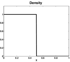
Refer to caption
Refer to caption
Refer to caption
Refer to caption
Figure 1: Moment dynamics for a free boundary connecting areas where e=0𝑒0e=0 and e>0𝑒0e>0. Initial conditions. Top-left: M0subscript𝑀0M_{0}. Top-right: M1subscript𝑀1M_{1}, Bottom-left: weights. Bottom-right: abscissas. The solid line corresponds to (ρ1,v1subscript𝜌1subscript𝑣1\rho_{1},v_{1}), the dashed line with circles to (ρ2,v2subscript𝜌2subscript𝑣2\rho_{2},v_{2}).

The ground difference with the first test case is that the transition between the two zones is smooth, and so the numerical strategy to account for this transition is important. The analytical solution of this problem, in smooth areas, consists of a decoupled transport of each of the quadrature nodes as two independant pressureless gas as showed in system (3.14). This comes from the fact that the number of Dirac delta functions reconstructed from the moments, two in this case, is always sufficient to capture the problem dynamics. The equivalence between the kinetic and macroscopic equations is preserved, and the solution in terms of moments satisfies the entropy equation. Therefore, the solution is the superposition of a translation at constant velocity v2=1subscript𝑣21v_{2}=1, and a transport with the following velocity field:

v1={1x[0, 0.1]1+x0.10.3x[0.1, 0.4]2x[0.4, 0.5]subscript𝑣1cases1𝑥00.11𝑥0.10.3𝑥0.10.42𝑥0.40.5v_{1}=\left\{\begin{array}[]{cc}1&x\in[0,\,0.1]\\ 1+\frac{x-0.1}{0.3}&x\in[0.1,\,0.4]\\ 2&x\in[0.4,\,0.5]\end{array}\right. (6.33)
Refer to caption
Refer to caption
Refer to caption
Refer to caption
Figure 2: Moment dynamics for a free boundary connecting areas where e=0𝑒0e=0 and e>0𝑒0e>0. Solution at t=0.2𝑡0.2t=0.2. Top-left: M0subscript𝑀0M_{0}. Top-right: M1subscript𝑀1M_{1}. Bottom-left: weights, Bottom-right:abscissas. The solid line corresponds to (ρ1,v1subscript𝜌1subscript𝑣1\rho_{1},v_{1}), the dashed line with circles to (ρ2,v2subscript𝜌2subscript𝑣2\rho_{2},v_{2}).

The analytical solution, displayed in Fig.  2, has two fronts at x=0.2𝑥0.2x=0.2 and x=0.9𝑥0.9x=0.9 moving with a velocity v=1𝑣1v=1 and v=2𝑣2v=2 respectively. The first front corresponds to particles initiated with velocity v=1𝑣1v=1 between x=0𝑥0x=0 and x=0.1𝑥0.1x=0.1. The second front corresponds to particles initiated with velocity v=2𝑣2v=2 between x=0.4𝑥0.4x=0.4 and x=0.5𝑥0.5x=0.5. The square wave between x=0.8𝑥0.8x=0.8 and x=0.9𝑥0.9x=0.9 is the final location of the particles initiated with velocity v=2𝑣2v=2 between x=0.4𝑥0.4x=0.4 and x=0.5𝑥0.5x=0.5. The value of ρ1subscript𝜌1\rho_{1} between x=0.3𝑥0.3x=0.3 and x=0.8𝑥0.8x=0.8 corresponds to the expansion of the density field due to transport with a linear velocity field with positive slope. The value of the density in that area is the solution of the equation tρ1+v1xρ1=ρ1xv1subscript𝑡subscript𝜌1subscript𝑣1subscript𝑥subscript𝜌1subscript𝜌1subscript𝑥subscript𝑣1\partial_{t}\rho_{1}+v_{1}\partial_{x}\rho_{1}=-\rho_{1}\partial_{x}v_{1}, which yields ρ1=0.3subscript𝜌10.3\rho_{1}=0.3 at time t=0.2𝑡0.2t=0.2 444In the interval [0.8,0.9]0.80.9[0.8,0.9], although ρ2subscript𝜌2\rho_{2} should be null (the square wave at velocity v2=1subscript𝑣21v_{2}=1 should be bounded between the front x=0.2𝑥0.2x=0.2 and x=0.7𝑥0.7x=0.7) we computed ρ2=0.5subscript𝜌20.5\rho_{2}=0.5 and v2=2subscript𝑣22v_{2}=2. This is consistent with the conditions in Section  2.3 for moment vectors at the frontier of the moment space..

According to the initial conditions, both weights have the same profile, the quantities q/(M0e)𝑞subscript𝑀0𝑒{q}/{(M_{0}\,e)} and q/e3/2𝑞superscript𝑒32{q}/{e^{3/2}} are null. At time t=0.2𝑡0.2t=0.2, the weight profiles are different in the interval [0.3,0.8]0.30.8[0.3,0.8] corresponding to the expansion of ρ1subscript𝜌1\rho_{1}. Therefore, q/e3/2𝑞superscript𝑒32{q}/{e^{3/2}} is non null, as well as qM0e𝑞subscript𝑀0𝑒\frac{q}{M_{0}e}, since the velocities have also different values, and can be exactly calculated (see Fig. 12).

7 Numerical simulations via kinetic schemes

This section is devoted to the discretization of (2.3)-(2.5)-(2.6). As already stated, we use as a building block a natural first-order kinetic scheme already proposed in the literature [Jin & Li (2003), Gosse et al. (2003), Desjardins et al. (2008)] and briefly recalled here for the sake of completeness.

Let us first introduce a time step Δt>0Δ𝑡0\Delta t>0 and a space step Δx>0Δ𝑥0\Delta x>0 that we assume to be constant for simplicity. We set λ=Δt/Δx𝜆Δ𝑡Δ𝑥\lambda={\Delta t}/{\Delta x} and define the mesh interfaces xj+1/2=jΔxsubscript𝑥𝑗12𝑗Δ𝑥x_{j+1/2}=j\Delta x for j𝑗j\in\mathbb{Z}, and the intermediate times tn=nΔtsuperscript𝑡𝑛𝑛Δ𝑡t^{n}=n\Delta t for n𝑛n\in\mathbb{N}. In the sequel, 𝐌jnsubscriptsuperscript𝐌𝑛𝑗{\bf M}^{n}_{j} denotes the approximate value of 𝐌𝐌{\bf M} at time tnsuperscript𝑡𝑛t^{n} and on the cell 𝒞j=[xj1/2,xj+1/2)subscript𝒞𝑗subscript𝑥𝑗12subscript𝑥𝑗12\mathcal{C}_{j}=[x_{j-1/2},x_{j+1/2}). For n=0𝑛0n=0, we set 𝐌j0=1Δxxj1/2xj+1/2𝐌0(x)𝑑x,jformulae-sequencesubscriptsuperscript𝐌0𝑗1Δ𝑥superscriptsubscriptsubscript𝑥𝑗12subscript𝑥𝑗12subscript𝐌0𝑥differential-d𝑥𝑗{\bf M}^{0}_{j}=\frac{1}{\Delta x}\int_{x_{j-1/2}}^{x_{j+1/2}}{\bf M}_{0}(x)dx,\quad j\in\mathbb{Z}, where 𝐌0(x)subscript𝐌0𝑥{\bf M}_{0}(x) is the initial condition.
Let us now assume as given (𝐌jn)jsubscriptsubscriptsuperscript𝐌𝑛𝑗𝑗({\bf M}^{n}_{j})_{j\in\mathbb{Z}} the sequence in ΩΩ\Omega of approximate values at time tnsuperscript𝑡𝑛t^{n}. In order to advance it to the next time level tn+1superscript𝑡𝑛1t^{n+1}, the kinetic scheme is decomposed into two steps.
 
First step : transport (tntn+1superscript𝑡𝑛superscript𝑡𝑛limit-from1t^{n}\to t^{n+1-})
We first set 𝐔jn=𝐔(𝐌jn)subscriptsuperscript𝐔𝑛𝑗𝐔subscriptsuperscript𝐌𝑛𝑗{\bf U}^{n}_{j}={\bf U}({\bf M}^{n}_{j}) and define the function (x,v)fn(x,v)𝑥𝑣superscript𝑓𝑛𝑥𝑣(x,v)\to{f}^{n}(x,v) by

fn(x,v)=(ρ1)jnδ(v(v1)jn)+(ρ2)jnδ(v(v2)jn),(x,v)𝒞j×,j.formulae-sequencesuperscript𝑓𝑛𝑥𝑣subscriptsuperscriptsubscript𝜌1𝑛𝑗𝛿𝑣subscriptsuperscriptsubscript𝑣1𝑛𝑗subscriptsuperscriptsubscript𝜌2𝑛𝑗𝛿𝑣subscriptsuperscriptsubscript𝑣2𝑛𝑗formulae-sequencefor-all𝑥𝑣subscript𝒞𝑗𝑗{f}^{n}(x,v)=(\rho_{1})^{n}_{j}\delta\big{(}v-(v_{1})^{n}_{j}\big{)}+(\rho_{2})^{n}_{j}\delta\big{(}v-(v_{2})^{n}_{j}\big{)},\quad\forall\,\,(x,v)\in\mathcal{C}_{j}\times\mathbb{R},\,\,\,j\in\mathbb{Z}.

We then solve the transport equation

{tf+vxf=0,(x,v)×,f(t=0,x,v)=fn(x,v),casesformulae-sequencesubscript𝑡𝑓𝑣subscript𝑥𝑓0𝑥𝑣𝑓𝑡0𝑥𝑣superscript𝑓𝑛𝑥𝑣\left\{\begin{array}[]{l}\partial_{t}f+v\partial_{x}f=0,\quad(x,v)\in\mathbb{R}\times\mathbb{R},\\ f(t=0,x,v)=f^{n}(x,v),\end{array}\right. (7.34)

the solution of which is given by f(t,x,v)=fn(xvt,v)𝑓𝑡𝑥𝑣superscript𝑓𝑛𝑥𝑣𝑡𝑣f(t,x,v)=f^{n}(x-vt,v).
At last, we set fn+1(x,v)=fn(xvΔt,v)superscript𝑓𝑛limit-from1𝑥𝑣superscript𝑓𝑛𝑥𝑣Δ𝑡𝑣{f}^{n+1-}(x,v)=f^{n}(x-v\Delta t,v).
 
Second step : collapse (tn+1tn+1superscript𝑡𝑛limit-from1superscript𝑡𝑛1t^{n+1-}\to t^{n+1})
The first four moments at time tn+1superscript𝑡𝑛1t^{n+1} are now naturally defined by setting

(Mi)jn+1=1Δxxj1/2xj+1/2+vifn+1(x,v)𝑑v𝑑x.subscriptsuperscriptsubscript𝑀𝑖𝑛1𝑗1Δ𝑥superscriptsubscriptsubscript𝑥𝑗12subscript𝑥𝑗12superscriptsubscriptsuperscript𝑣𝑖superscript𝑓𝑛limit-from1𝑥𝑣differential-d𝑣differential-d𝑥(M_{i})^{n+1}_{j}=\frac{1}{\Delta x}\int_{x_{j-1/2}}^{x_{j+1/2}}\int_{-\infty}^{+\infty}v^{i}{f}^{n+1-}(x,v)dvdx.

Then, we have 𝐌jn+1=((M0)jn+1,(M1)jn+1,(M2)jn+1,(M3)jn+1)tsubscriptsuperscript𝐌𝑛1𝑗superscriptsubscriptsuperscriptsubscript𝑀0𝑛1𝑗subscriptsuperscriptsubscript𝑀1𝑛1𝑗subscriptsuperscriptsubscript𝑀2𝑛1𝑗subscriptsuperscriptsubscript𝑀3𝑛1𝑗𝑡{\bf M}^{n+1}_{j}=\big{(}(M_{0})^{n+1}_{j},(M_{1})^{n+1}_{j},(M_{2})^{n+1}_{j},(M_{3})^{n+1}_{j}\big{)}^{t} for all j𝑗j\in\mathbb{Z}, which completes the algorithm description.

Remark 1.

It is easy to see that this scheme preserves the moment space ΩΩ\Omega, see for instance [Desjardins et al. (2008)].

Remark 2.

Under the natural CFL condition Δtmaxj((v1)jn,(v2)jn)CFLΔxΔ𝑡subscript𝑗subscriptsuperscriptsubscript𝑣1𝑛𝑗subscriptsuperscriptsubscript𝑣2𝑛𝑗𝐶𝐹𝐿Δ𝑥{\Delta t}\,\max_{j\in\mathbb{Z}}((v_{1})^{n}_{j},(v_{2})^{n}_{j})\leq CFL\,\Delta x, with CFL1𝐶𝐹𝐿1CFL\leq 1, integrating (7.34) over (t,x,v)(0,Δt)×𝒞j×𝑡𝑥𝑣0Δ𝑡subscript𝒞𝑗(t,x,v)\in(0,\Delta t)\times\mathcal{C}_{j}\times\mathbb{R} and against visuperscript𝑣𝑖v^{i}, i=0,,3𝑖03i=0,...,3 easily leads to the equivalent update formula

𝐌jn+1=𝐌jnΔtΔx(𝐅j+1/2n𝐅j1/2n),j,formulae-sequencesubscriptsuperscript𝐌𝑛1𝑗subscriptsuperscript𝐌𝑛𝑗Δ𝑡Δ𝑥subscriptsuperscript𝐅𝑛𝑗12subscriptsuperscript𝐅𝑛𝑗12𝑗{\bf M}^{n+1}_{j}={\bf M}^{n}_{j}-\frac{\Delta t}{\Delta x}\big{(}{\bf F}^{n}_{j+1/2}-{\bf F}^{n}_{j-1/2}\big{)},\quad j\in\mathbb{Z},

where we have set 𝐅j+1/2n=((M1)j+1/2n,(M2)j+1/2n,(M3)j+1/2n,(M4)j+1/2n)tsubscriptsuperscript𝐅𝑛𝑗12superscriptsubscriptsuperscriptsubscript𝑀1𝑛𝑗12subscriptsuperscriptsubscript𝑀2𝑛𝑗12subscriptsuperscriptsubscript𝑀3𝑛𝑗12subscriptsuperscriptsubscript𝑀4𝑛𝑗12𝑡{\bf F}^{n}_{j+1/2}=\big{(}(M_{1})^{n}_{j+1/2},(M_{2})^{n}_{j+1/2},(M_{3})^{n}_{j+1/2},(M_{4})^{n}_{j+1/2}\big{)}^{t} and (Mi)j+1/2n=(Mi)j+1/2n++(Mi)j+1/2nsubscriptsuperscriptsubscript𝑀𝑖𝑛𝑗12subscriptsuperscriptsubscript𝑀𝑖limit-from𝑛𝑗12subscriptsuperscriptsubscript𝑀𝑖limit-from𝑛𝑗12(M_{i})^{n}_{j+1/2}=(M_{i})^{n+}_{j+1/2}+(M_{i})^{n-}_{j+1/2}, and with

(Mi)j+1/2n=(ρ1)j+1nmin(0,(v1)j+1n)((v1)j+1n)i1+min(0,(v2)j+1n)(ρ2)j+1n((v2)j+1n)i1,subscriptsuperscriptsubscript𝑀𝑖limit-from𝑛𝑗12subscriptsuperscriptsubscript𝜌1𝑛𝑗10subscriptsuperscriptsubscript𝑣1𝑛𝑗1superscriptsubscriptsuperscriptsubscript𝑣1𝑛𝑗1𝑖10subscriptsuperscriptsubscript𝑣2𝑛𝑗1subscriptsuperscriptsubscript𝜌2𝑛𝑗1superscriptsubscriptsuperscriptsubscript𝑣2𝑛𝑗1𝑖1(M_{i})^{n-}_{j+1/2}=(\rho_{1})^{n}_{j+1}\min(0,(v_{1})^{n}_{j+1})\big{(}(v_{1})^{n}_{j+1}\big{)}^{i-1}+\min(0,(v_{2})^{n}_{j+1})(\rho_{2})^{n}_{j+1}\big{(}(v_{2})^{n}_{j+1}\big{)}^{i-1},
(Mi)j+1/2n+=(ρ1)jnmax(0,(v1)j+1n)((v1)jn)i1+(ρ2)jnmax(0,(v2)j+1n)((v2)jn)i1.subscriptsuperscriptsubscript𝑀𝑖limit-from𝑛𝑗12subscriptsuperscriptsubscript𝜌1𝑛𝑗0subscriptsuperscriptsubscript𝑣1𝑛𝑗1superscriptsubscriptsuperscriptsubscript𝑣1𝑛𝑗𝑖1subscriptsuperscriptsubscript𝜌2𝑛𝑗0subscriptsuperscriptsubscript𝑣2𝑛𝑗1superscriptsubscriptsuperscriptsubscript𝑣2𝑛𝑗𝑖1(M_{i})^{n+}_{j+1/2}=(\rho_{1})^{n}_{j}\max(0,(v_{1})^{n}_{j+1})\big{(}(v_{1})^{n}_{j}\big{)}^{i-1}+(\rho_{2})^{n}_{j}\max(0,(v_{2})^{n}_{j+1})\big{(}(v_{2})^{n}_{j}\big{)}^{i-1}.

7.1 Numerical quadrature strategy at the frontier of the moment space

This paragraph addresses the issue of how to numerically handle the transition between a vector in the interior of the moment space, and a vector lying at its frontier. For an isolated point at the frontier of the moment space ΓΓ\Gamma, there is no specific problem since we use a single quadrature node and the quadrature is not a problem. The two problems we have to face are related to the preservation of the cone in which we envision to work in section 2 as well as to deal with finite precision algebra in the neighborhood of the point (0,0)00(0,0) in the (e,q)𝑒𝑞(e,q) plane.

Consequently we introduce two constants in the numerical quadrature we use. First, for finite precision algebra and in order to avoid numerical errors, we only evaluate the two quadrature nodes when e/M02>ϵ1𝑒superscriptsubscript𝑀02subscriptitalic-ϵ1e/M_{0}^{2}>\epsilon_{1}, where ϵ1subscriptitalic-ϵ1\epsilon_{1} is a small number related to machine precision. Under this threshold, the velocity dispersion is considered null (e=0𝑒0e=0), and the set of Dirac delta functions are reconstructed as suggested in section 222: ρ1=ρ2=M0/2subscript𝜌1subscript𝜌2subscript𝑀02\rho_{1}=\rho_{2}=M_{0}/2, v1=v2=M1/M0subscript𝑣1subscript𝑣2subscript𝑀1subscript𝑀0v_{1}=v_{2}=M_{1}/M_{0}.

Refer to caption
Figure 3: Handling of the moment space border with the admissible cone.

Secondly, since we want to deal with compactly supported velocity distribution at the kinetic level, we will introduce another constant, η𝜂\eta which is a bound for the distance between the two abscissas. In fact we would like to impose to the solution to remain inside the cone in the (e,q)𝑒𝑞(e,q) plane : |q|M0eη𝑞subscript𝑀0𝑒𝜂\frac{|q|}{M_{0}e}\leq\eta. It will be shown in the following examples that the cone is in fact automatically preserved by the proposed algorithm and that such a bound does not have to be imposed but is satisfied by the numerical solution.

If |q|M0e>η𝑞subscript𝑀0𝑒𝜂\frac{|q|}{M_{0}e}>\eta, then we set q/(M0e)=sign(q)η𝑞subscript𝑀0𝑒𝑠𝑖𝑔𝑛𝑞𝜂q/(M_{0}e)=sign(q)\,\eta, so that :

qM0e=sign(q)η,q=sign(q)ηM0e,M3=q+M1M2/M0.formulae-sequence𝑞subscript𝑀0𝑒𝑠𝑖𝑔𝑛𝑞𝜂formulae-sequence𝑞𝑠𝑖𝑔𝑛𝑞𝜂subscript𝑀0𝑒subscript𝑀3𝑞subscript𝑀1subscript𝑀2subscript𝑀0\frac{q}{M_{0}e}=sign(q)\,\eta,\quad q=sign(q)\,\eta\,M_{0}\,e,\qquad M_{3}=q+M_{1}M_{2}/M_{0}.

As illustrated in Fig 3 and explained in Section  2.3, the variable q𝑞q naturally lives in a cone delimited by the straight lines of slope ±ηplus-or-minus𝜂\pm\eta and becomes null when eϵ1𝑒subscriptitalic-ϵ1e\leq\epsilon_{1}.

Let us remark that limiting qM0e𝑞subscript𝑀0𝑒\frac{q}{M_{0}e} does not lead to a limitation on the quantity qe3/2𝑞superscript𝑒32\frac{q}{e^{3/2}} in such a way as to allow the possibility to reach large ratio in terms of weights (one weight can approach a zero value while the quantity qe3/2𝑞superscript𝑒32\frac{q}{e^{3/2}} grows indefinitely) but without allowing the abscissas distance to grow beyond of fixed limit naturally inherited from the initial solutions at the kinetic level. We will come back to this point in the following result section. For the simulations we present, the parameters are such that: ϵ1=109subscriptitalic-ϵ1superscript109\epsilon_{1}=10^{-9} and η=2𝜂2\eta=2.

7.2 Numerical results

This section is devoted to numerical illustrations of the two Riemann problems and one dedicated to the case of a free boundary connecting zone where e=0𝑒0e=0 and a zone where e>0𝑒0e>0, discussed in Section 666.

In all the figures, we choose to represent ρ1subscript𝜌1\rho_{1} and v1subscript𝑣1v_{1} by solid lines, and ρ2subscript𝜌2\rho_{2} and v2subscript𝑣2v_{2} by lines with circle markers. In the representation of weights and abscissas, values have to be assigned for v1subscript𝑣1v_{1} and v2subscript𝑣2v_{2} : we thus decide that v1subscript𝑣1v_{1} is the maximum of the relative values of velocity.

Two packet collision

Figure 4 represents the initial conditions for the two particle packet case. Figures 5 and 6 presents the numerical and analytical solutions for the two particle packet case with ρL=ρR=1subscript𝜌𝐿subscript𝜌𝑅1\rho_{L}=\rho_{R}=1, and vL=1subscript𝑣𝐿1v_{L}=1, vR=1subscript𝑣𝑅1v_{R}=-1. The computation is run with a 100010001000 cell grid on the spatial domain [0,1]01[0,1], with CFL=1𝐶𝐹𝐿1CFL=1. The length of each packet is 0.40.40.4 (ρ1=ρ2=v1=v2=0subscript𝜌1subscript𝜌2subscript𝑣1subscript𝑣20\rho_{1}=\rho_{2}=v_{1}=v_{2}=0 for x0.1𝑥0.1x\leq 0.1 and x0.9𝑥0.9x\geq 0.9) and the two packets start to collide exactly at time t=0𝑡0t=0. Moving in opposite direction one across the other, with the same opposite speed, they then overlay and we note in particular that ρ1=ρ2=1subscript𝜌1subscript𝜌21\rho_{1}=\rho_{2}=1 and v1=v2=0subscript𝑣1subscript𝑣20v_{1}=v_{2}=0 in the mixing zone (see for instance the plots at time t=0.1𝑡0.1t=0.1). As expected, they finally get separated again and we note that a perfect agreement is obtained with the exact entropic solution.
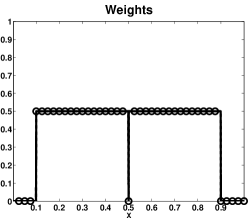
Refer to caption
Refer to caption
Figure 4: Initial fields of weights (left) and abscissas (right) for the two particle packet case. The first quadrature node is represented by solid lines whereas the second node is represented by circles.
Refer to caption
Refer to caption
Refer to caption
Refer to caption
Refer to caption
Refer to caption
Figure 5: Results for the two packet case at time t=0.1𝑡0.1t=0.1. Top: Numerical results for M0subscript𝑀0M_{0} (solid line) and M1subscript𝑀1M_{1} (dashed line) (left) and for M2subscript𝑀2M_{2} (solid line) and M3subscript𝑀3M_{3} (dashed line) (right). Middle: Analytical result for weights (left) and abscissas (right). Bottom: Numerical results for weights (left) and abscissas (right). The solid line corresponds to the higher abscissa, the dashed line with circle to the lower one.
Refer to caption
Refer to caption
Refer to caption
Refer to caption
Figure 6: Results for the two packet case at time t=0.4𝑡0.4t=0.4. Top: Analytical result for weights (left) and abscissas (right). Bottom: Numerical results for weights (left) and abscissas (right). The solid line corresponds to the higher abscissa, the dashed line with circle to the lower one.

Four packet collision

Figures 7 presents the initial conditions. Figures  8 and 10 present the numerical and analytical solutions respectively for the moments and the weights and abscissas. The computation is run with a 100010001000 cell grid on the spatial domain [0,1]01[0,1], at CFL=1𝐶𝐹𝐿1CFL=1. Here, we observe the presence of two Dirac delta functions as already discussed in Section 6. The agreement between exact and numerical solutions for the moments is very good, showing that the numerical solution converges to the analytical one. The disparities encountered between the analytical and numerical solution in the case of the weights and abscissas are due to the fact that the mapping 𝐔(𝐌)𝐔𝐌{\bf U}({\bf M}) is discontinuous at the moment space border. In area of numerical diffusion (x0.22𝑥0.22x\approx 0.22 and x0.88𝑥0.88x\approx 0.88), when the dispersion e𝑒e is under the threshold ϵ1subscriptitalic-ϵ1\epsilon_{1}, weights and abscissas are reconstructed as explained in section 222.

The wave propagating at velocity 1.21.21.2 and separating the constant states (v1=0.8,v2=0formulae-sequencesubscript𝑣10.8subscript𝑣20v_{1}=0.8,v_{2}=0) and (v1=1.2,v2=0.8formulae-sequencesubscript𝑣11.2subscript𝑣20.8v_{1}=1.2,\,v_{2}=0.8) is steep and coincide with the analytical wave whereas the wave propagating at velocity 0.80.80.8 is actually smooth since the CFL number is based on the highest value of velocity, which is 1.21.21.2 in this studied case. The same explanation holds for the symmetric jump at location x=0.78𝑥0.78x=0.78. Meanwhile, because of the conservation of the velocity moments, the numerical velocity jump (at x=0.154𝑥0.154x=0.154) happens before the analytical velocity jump (at x=0.18𝑥0.18x=0.18). One can here notice that the quadrature method provides the expected value of velocity in the numerical diffusion zones. The same explanation holds for the different velocity jump locations between the analytical and numerical solution at x=0.82𝑥0.82x=0.82 and x=0.845𝑥0.845x=0.845. The same phenomenon is responsible for the disparities between the analytical and numerical solutions at the δ𝛿\delta-shocks locations, at x=0.4𝑥0.4x=0.4 and x=0.6𝑥0.6x=0.6.

Figure  9 displays the final profile of the quantities qM0e𝑞subscript𝑀0𝑒\frac{q}{M_{0}e} and qe3/2𝑞superscript𝑒32\frac{q}{e^{3/2}}. Thus, qM0e𝑞subscript𝑀0𝑒\frac{q}{M_{0}e} has significative values in areas where the abscissa distance as well as the weight difference are important, whereas qe3/2𝑞superscript𝑒32\frac{q}{e^{3/2}} reaches high value in areas where the weight ratio is important. Since in the domain, except for the singularities, the weights have the same value, both quantities are equal to zero. At the singularities, qe3/2𝑞superscript𝑒32\frac{q}{e^{3/2}} is roughly proportional to the square root of the weight ratio, and qM0e𝑞subscript𝑀0𝑒\frac{q}{M_{0}e} is bounded, accounting for the fact that the velocity field is bounded.
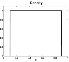
Refer to caption
Refer to caption
Refer to caption
Refer to caption
Figure 7: Four packet case with ρL=ρR=1subscript𝜌𝐿subscript𝜌𝑅1\rho_{L}=\rho_{R}=1, and v1=1.2subscript𝑣11.2v_{1}=1.2, v2=0.8subscript𝑣20.8v_{2}=0.8. Initial conditions. Top: M0subscript𝑀0M_{0} (left) and M1subscript𝑀1M_{1} (right). Bottom: weights (left) and abscissas (right). The solid line corresponds to the set (ρ1,v1subscript𝜌1subscript𝑣1\rho_{1},v_{1}), and the dashed line with circles to the set (ρ2,v2subscript𝜌2subscript𝑣2\rho_{2},v_{2}).
Refer to caption
Refer to caption
Refer to caption
Refer to caption
Figure 8: Four packet case. Results at t=0.1𝑡0.1t=0.1. Analytical (solid line) and numerical (dashed line with circles) solutions. Top: M0subscript𝑀0M_{0} (left) and M1subscript𝑀1M_{1} (right). Bottom: M2subscript𝑀2M_{2} (left) and M3subscript𝑀3M_{3} (right).
Refer to caption
Refer to caption
Figure 9: Four particle packet case, at time t=0.1𝑡0.1t=0.1. Left: ratio q/(M0e)𝑞subscript𝑀0𝑒q/(M_{0}e). Right: ratio q/e3/2𝑞superscript𝑒32q/e^{3/2}.
Refer to caption
Refer to caption
Refer to caption
Refer to caption
Figure 10: Four packet case. Results at t=0.1𝑡0.1t=0.1. Top: Analytical weights (left) and abscissas (right). Bottom: Numerical weights (left) and abscissas (right). The solid line corresponds to the set (ρ1,v1subscript𝜌1subscript𝑣1\rho_{1},v_{1}), and the dashed line with circles to the set (ρ2,v2subscript𝜌2subscript𝑣2\rho_{2},v_{2}).

We have thus provided numerical simulations in the two cases for which we have at our disposal an analytical entropic solution, either in the piecewise contant case, or in the singular case where δ𝛿\delta-shock mesure solutions are present. In the first case, the crossing of the two droplets monokinetic packets is very properly reproduced without numerical diffusion since we work at CFL one, even if this is not symptomatic of the numerical diffusion such methods will encounter with a first order method in realistic configurations [Kah et al. (2010)]. In the second case, the numerical method is able to capture the creation of the measure singular solutions associated to the fact the we have limited the number of quadrature node to two. With this node number limitation, the proper physical solution, in the infinite Knudsen number limit, where the various droplet packets cross without interacting, differs from the entropic solution of the system of partial differential equations (2.2) obtained through the quadrature-based closure. This is the same type of behavior as seen in the case of pressureless gas dynamics at a lower level.

Free boundary case

The last test case, explained in subsection  6.3, assesses the ability of the method to solve free boundary cases connecting in a continuous manner states lying in the interior of the moment space and at its frontier. The chosen grid contains 400400400 cells, CFL number is set to 0.980.980.98. This value of the CFL number is chosen is order to prevent high frequency instabilities to occur. The computation is run until t=0.2𝑡0.2t=0.2. The analytical solution has been provided in subsection  6.3.

Results are displayed in Fig.  11. Let us first focus on the fronts present at x=0.2𝑥0.2x=0.2 and x=0.9𝑥0.9x=0.9 for the analytical solution. Since the CFL number is based on the highest velocity value (222 in this case) and is taken as 0.980.980.98, the corresponding wave is less diffused at x=0.9𝑥0.9x=0.9, contrary to the front wave located at x=0.2𝑥0.2x=0.2 moving at velocity v2=1subscript𝑣21v_{2}=1. Note that in these areas, ρ1=ρ2subscript𝜌1subscript𝜌2\rho_{1}=\rho_{2}, since e=0𝑒0e=0 or e<ϵ1𝑒subscriptitalic-ϵ1e<\epsilon_{1}. The borders of these areas are clearly seen at x0.28𝑥0.28x\approx 0.28 and x=0.8𝑥0.8x=0.8. The constant profiles for ρ2subscript𝜌2\rho_{2} and ρ1subscript𝜌1\rho_{1} observed respectively between x=0.5𝑥0.5x=0.5 and x=0.7𝑥0.7x=0.7 and between x=0.5𝑥0.5x=0.5 and x=0.8𝑥0.8x=0.8 correspond to the one observed in the analytical solution. In the area between x=0.28𝑥0.28x=0.28 and x=0.5𝑥0.5x=0.5, the density profiles would be expected to be constant, with the same value as before. Instead of that, one observes a peak value for ρ2subscript𝜌2\rho_{2} and a low value for ρ1subscript𝜌1\rho_{1}, the sum ρ1+ρ2subscript𝜌1subscript𝜌2\rho_{1}+\rho_{2} being constant. This results from a coupling between the behaviour of the quadrature method when e𝑒e tends to zero and the numerical diffusion. We are here in the situation q>0𝑞0q>0 and e𝑒e small but e>ϵ1𝑒subscriptitalic-ϵ1e>\epsilon_{1}. See Lemma 2.4. Further away from the discontinuities the density values tend to their analytical value.
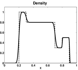
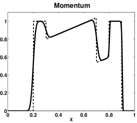
Refer to caption
Refer to caption
Refer to caption
Refer to caption
Figure 11: Moment dynamics for a free boundary connecting areas where e=0𝑒0e=0 and e>0𝑒0e>0. Results at t=0.2𝑡0.2t=0.2. Top: Analytical (dashed line) and numerical (solid line) density (left) and momentum (right). Bottom: weights (left) and abscissas (right). The solid line corresponds to the set (ρ1,v1subscript𝜌1subscript𝑣1\rho_{1},v_{1}), and the dashed line with circles to the set (ρ2,v2subscript𝜌2subscript𝑣2\rho_{2},v_{2}).
Refer to caption
Refer to caption
Figure 12: Moment dynamics for a free boundary connecting areas where e=0𝑒0e=0 and e>0𝑒0e>0. Results at t=0.2𝑡0.2t=0.2. Left: ratio q/(M0e)𝑞subscript𝑀0𝑒q/(M_{0}e). The dashed line with crosses represents the analytical solution, whereas the solid line represents the numerical solution, bounded by its extremal initial values (dotted-dashed curve). Right: ratio q/e3/2𝑞superscript𝑒32q/e^{3/2}.

Figure 12 displays the profile of quantities qM0e𝑞subscript𝑀0𝑒\frac{q}{M_{0}e} and qe3/2𝑞superscript𝑒32\frac{q}{e^{3/2}} at time t=0.2𝑡0.2t=0.2. First, it is interesting to note that qM0e𝑞subscript𝑀0𝑒\frac{q}{M_{0}e} is naturally bounded by 111 in the numerical simulation, as shown in Fig  12 such that the bound imposed with η=2𝜂2\eta=2 in never effective. Let us underline that in the present case, the numerical scheme allows to preserve the proposed cone associated with a maximal distance between the abscissas which is also invariant. Comparing the analytical value of |q/(M0e)|𝑞subscript𝑀0𝑒|q/(M_{0}\,e)| to the numerical resolution in Fig. 12, it is instructive to observe that the numerical diffusion is creating zones where it can be far from zero, whereas it should be zero in the analytical solution. However, this is done is such a way as to preserve the maximal value foreseen as the maximal distance between the abscissa at time t=0𝑡0t=0 which is one. Let us also underline that we have rerun this case with various values of ϵ1subscriptitalic-ϵ1\epsilon_{1} varying from 109superscript10910^{-9} up to 107superscript10710^{-7} without any effect on the solution. It can also be noticed that the quantity q/e3/2𝑞superscript𝑒32q/e^{3/2} has large values in the regions of connection between the interior and the frontier of the moment space, but has no reason to be naturally limited as opposed to the previous quantity as it can be seen in Fig. 11-bottom left.

Concerning the convergence behavior of the numerical solution, we display the error in L1subscript𝐿1L_{1} norm relative to the analytical solution to assess convergence quantitatively, Tab 1, for 400400400, 800800800, 160016001600, and 320032003200 cell grids. As expected, we get an experimental order of convergence of 0.50.50.5. These data clearly show the convergence towards the analytical solution for each moment.

As a consequence, it can be seen that we have designed the proper theoretical setting for the transition from the interior of the moment space towards its frontier since the cone we have defined seems to be automatically preserved by the kinetic scheme we have used. Such a point would be worth a detailed study which is beyond the scope of the present paper.

Grid size 400400400 800800800 160016001600 320032003200
m0subscript𝑚0m_{0} 0.049 0.0344 0.0244 0.0172
m1subscript𝑚1m_{1} 0.0442 0.0307 0.0219 0.0153
m2subscript𝑚2m_{2} 0.0396 0.0271 0.0195 0.0136
m3subscript𝑚3m_{3} 0.0362 0.0244 0.0177 0.0122
Table 1: L1subscript𝐿1L_{1} error on moments relative to the analytical solution.

8 Conclusion

In this paper, we have extended the notion of entropic measure solution of quadrature-based moment method for kinetic equations. Such kinetic equations are frequently encountered in many application fields where a complex dynamics in phase space is involved. Following the contribution of [Bouchut & al (2003)] for the pressureless gas dynamics which is the one-node quadrature version of a more general system of conservation laws for quadrature-based moment models, we have been able to provide a few problem test-cases showing that the numerical solution of the resulting system of conservation laws through kinetic schemes reproduces the defined entropic solution as well as the proper theoretical setting for the transition from the interior to the frontier of the moment space. It is an important point for the case of PTC where the solution remains smooth and where the scheme allows to describe the phase space dynamics properly as well as for cases where the complexity of the dynamics in phase space leads to generalized δ𝛿\delta-shocks, as observed for pressureles gas dynamics due to the weakly hyperbolic structure of the system of conservation laws. Two stumbling blocks still remains to be treated. First, we would need a uniqueness theory and a convergence analysis in a general framework in order to fully justify the use of the kinetic schemes for the simulation of such models. However, as explained already in [Bouchut (1994)], the framework of entropic solution is not sufficient in order to provide uniqueness since one can exhibit multiple entropic solutions for measure solutions. Let us underline that it is easy to construct the same type of measure solutions for system (2.3), which is the exact same collision case used by Bouchut, but with a motionless Dirac delta function in density localized at the collision point of the other two incoming “particles”. An infinite set of entropic solution can then be exhibited depending on the nature of the collision. As a consequence, it would be first useful to investigate such a point on the pressureless gas dynamics and then to extend it to the present system of higher order quadrature-based moment models. Besides, the construction of fully high order methods is still an open question and requires further developments.
At last, let us mention that most of the results of the present paper do naturally extend to higher order moment systems, but at the price of algebra complications. In fact, the key point lies in the extension of the proposed study of the behavior of the quadrature at the frontier of the moment space, namely when the two velocities v1subscript𝑣1v_{1} and v2subscript𝑣2v_{2} become equal. If we consider for instance the 666-moment model and assume that one of the three velocities v1subscript𝑣1v_{1}, v2subscript𝑣2v_{2} and v3subscript𝑣3v_{3} is smooth while the other two become equal, we are in the same framework as in the present paper. But the case when the three velocities tend to be equal needs to be precised in a future work.

Acknowledgement. We would like to thank the referees for a very careful reading of the paper and for useful hints to improve and make complete the present work.

References

  • [Bouchut (1994)] Bouchut, F. On zero pressure gas dynamics. In Advances in kinetic theory and computing, World Sci. Publishing, River Edge (1994) 171-190
  • [Bouchut & al (2003)] Bouchut, F., Jin, S., Li, X. Numerical approximations of pressureless and isothermal gas dynamics, SIAM J. Num. Anal, 41 (2003) 135–158
  • [Brenier & Corrias (1998)] Y. Brenier and L. Corrias A kinetic formulation for multi-branch entropy solutions of scalar conservation laws, Ann. Inst. H. Poincaré Anal. Non Linéaire, 15, No. 2 (1998) 169–190
  • [de Chaisemartin (2009)] de Chaisemartin, S., Polydisperse evaporating spray turbulent dispersion: Eulerian model and numerical simulation, Ph.D. thesis, Ecole Centrale Paris, available in english at http://tel.archives-ouvertes.fr/tel-00443982/en/ (2009)
  • [de Chaisemartin & al (2008)] de Chaisemartin, S. Fréret, L., Kah, D., Laurent, F., Fox, R.O., Réveillon, J., Massot, M., Eulerian models for turbulent spray combustion with polydispersity and droplet crossing, C. R. Mecanique, 337, No. 6-7 (2009) 438–448
  • [Desjardins et al. (2008)] Desjardins, O., Fox, R. O. & Villedieu, P., A quadrature-based moment method for dilute fluid-particle flows, J. Comp. Phys., 227 (2008) 2514–2539
  • [Fox (2009)] Fox, R. O. Higher-order quadrature-based moment methods for kinetic equations, J. Comp. Phys., 228 (2009) 7771–7791
  • [Fréret & al (2008)] Fréret, L., Lacour, C., de Chaisemartin, S., Ducruix, S., Durox, D., Laurent, F., Massot, M.., Pulsated free jets with polydisperse spray injection: experiments and numerical simulations. Proceedings of the Comb. institute, 32, No. 2 (2009) 2215–2229
  • [Fréret et al. (2010)] Fréret, L. and Thomine, O. and Reveillon, J. and de Chaisemartin, S. and Laurent, F. and Massot, M., On the role of preferential segregation in flame dynamics in polydisperse evaporating sprays. Proceedings of the Summer Program 2010, Center for Turbulence Research, Stanford University (2010) 383–392.
  • [Gosse & Runborg (2005)] L. Gosse and O. Runborg, Finite moment problems and applications to multiphase computations in geometric optics. Commun. Math. Sci., 3, No. 3 (2005) 373–392.
  • [Gosse et al. (2003)] L. Gosse, S. Jin and X. Li, Two moment systems for computing multiphase semiclassical limits of the Schrödinger equation, Math. Models Methods Appl. Sci., 13, No. 12 (2003) 1689–1723
  • [Jin & Li (2003)] S. Jin and X. Li, Multi-phase computations of the semiclassical limit of the Schrödinger equation and related problems: Whitham vs Wigner, Physica D: Nonlinear Phenomena, 182, No. 1-2 (2003) 46–85
  • [Kah (2010)] Kah, D. Taking into account polydispersity in the framework of a coupled Euler-Lagrange approach for the modeling of liquid fuel injection in internal combustion engines, Ph.D. Thesis, Ecole Centrale Paris, available in English online on TEL, http://tel.archives-ouvertes.fr/tel-00618786 (2010)
  • [Kah et al. (2010)] Kah, D., Laurent, F., Fréret, L., de Chaisemartin, S., Fox, R. O., Reveillon, J. & Massot, M. Eulerian quadrature-based moment models for dilute polydisperse evaporating sprays, Flow, Turbulence and Combustion, 85, No. 3-4 (2010) 649–676
  • [Laurent (2002)] Laurent, F. Mathematical and numerical modeling of polydisperse spray flames, Ph.D. Thesis of the University of Lyon, http://tel.archives-ouvertes.fr/tel-00185806/en/ (2002)
  • [Massot & al (2009)] Massot, M., de Chaisemartin, S., Fréret, L., Kah, D., Laurent, F., Eulerian multi-fluid models: modeling and numerical methods, In Modelling and Computation of Nanoparticles in Fluid Flows, Lectures of the von Karman Institute. NATO RTO-EN-AVT-169, http://www.rta.nato.int/pubs/rdp.asp?RDP=RTO-EN-AVT-169 (2009) 1–86
  • [Runborg (2000)] Runborg, O. Some new results in multiphase geometrical optics, M2AN. Mathematical Modelling and Numerical Analysis, 34, No. 3 (1991) 1203–1231
  • [Vikas et al. (2010)] Vikas, V., Wang, Z. J., Passalacqua, A., & Fox, R. O. Realizable high-order finite-volume schemes for quadrature-based moment methods, J. Comp. Phys., 230, No. 13 (2011) 5328–5352
  • [Williams (1958)] Williams, F.A., Spray combustion and atomization, Physics of fluids, 1 (1958) 541–545
  • [Yuan & Fox (2010)] Yuan, C. & Fox, R. O., Conditional quadrature method of moments for kinetic equations J.  Comp. Phys, 230, No. 22 (2011) 8216–8246