Spin exchange interaction with tunable range between graphene quantum dots

Abstract

We study the spin exchange between two electrons localized in separate quantum dots in graphene. The electronic states in the conduction band are coupled indirectly by tunneling to a common continuum of delocalized states in the valence band. As a model, we use a two-impurity Anderson Hamiltonian which we subsequently transform into an effective spin Hamiltonian by way of a two-stage Schrieffer-Wolff transformation. We then compare our result to that from a Coqblin-Schrieffer approach as well as to fourth order perturbation theory.

I Introduction

Spins in quantum dots (QDs) are under intense investigation as a possible realization of a quantum bits (qubits).Loss1998 Among the currently most advanced solid-state structures are top-gate patterned two-dimensional electron gases in GaAs heterostructures.Hanson2007 However, in this host material hyperfine interaction between the spin of the electron and that of the atomic nuclei of the host material leads to relatively short coherence times. A promising way to circumvent this problem is the use of carbon as a host material for spin qubits. Natural carbon comprises 99% of the carbon isotope ${}^{12}\mathrm{C}$ which has no nuclear spin. This gives carbon based devices the advantage that decoherence due to hyperfine interaction is suppressed by the small abundance of nuclear spins. Carbon is also a relatively light element, therefore spin-orbit coupling is expected to be weaker than in GaAs. One can expect a significant improvement of spin coherence times in carbon based structures. Graphene, a truly two-dimensional carbon-based crystal Novoselov2004 ; Novoselov2005 ; Zhang2005 ; Geim2007 ; Katsnelson2007 seems to be an ideal host material for spin qubitsTrauzettel2007 ; Tombros2007 . It naturally created a perfect confinement of electrons in one dimension. Moreover, in contrast to carbon nanotubes,Sahoo2005 ; Shenoy2005 the ability to lithographically pattern graphene allows for a deterministic device preparation, which is necessary for scalability.Loss1998 Graphene has a very interesting electronic structure with a gapless and linear dispersion around the Fermi energy. Furthermore, the electronic eigenstates carry an additional internal degree of freedom, dubbed pseudospin, which is always aligned with the direction of the momentum. These properties imitate the behavior of relativistic chiral massless Dirac particles.Zhang2005 ; Novoselov2005 ; Katsnelson2006 These relativistic-like properties lead to the phenomenon of Klein tunneling,Klein1929 ; Katsnelson2006 which actually prohibits any electrostatical confinement of electrons, i.e. prohibits the formation of quantum dots.

Among the most promising ideas to overcome Klein tunneling is to use graphene nanoribbons or constrictions instead of extended graphene as host material,Trauzettel2007 ; Stampfer2008 ; Silvestrov2007 see Fig. 1. In clean graphene nanoribbons with armchair boundaries, the additional confinement can lead to the opening of a small energy gap at the Fermi energy.Brey2006 The size of the gap is indirectly proportional to the width of the ribbon. In the presence of such a gap, the pseudo-relativistic behavior of the charge carriers is lost, and the material resembles a regular gaped semiconductor, enabling electrostatic confinement.Trauzettel2007 Interestingly, experiments observe the formation of a gap irrespective of the boundary condition.Han2007 As a side effect, the sharp edges also lift the valley degeneracy in bulk graphene, which could suppress the Heisenberg spin interaction between the quantum dots.Trauzettel2007

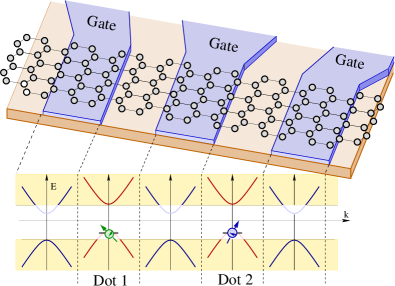
Figure 1: One-dimensional quantum dot array on an armchair graphene nanoribbon (drawing not to scale). Due to the ribbon structure, the dispersion relation of graphene can exhibit a gap, which scales inversely with the ribbon width. This gap allows for electrostatic confinement of electrons in quantum dots. As the bandgap is small compared to regular semiconductors, the spin exchange mechanism between the quantum dots is not dominated by RKKY-type processes alone, and superexchange processes contribute significantly.

Following Ref. Trauzettel2007, , we consider a system as shown in the upper part of Fig. 1 where several electric gates are placed on top of an armchair nanoribbon. By applying a gate voltage, the dispersion relation of the material below the gates can be shifted in energy, see the lower part of Fig. 1. If at a certain energy extended states could exist in one section, but not in the neighboring ribbon sections, additional size quantization along the ribbon leads to single localized states. In the energy interval above and below the gap, the states are extended and form a continuum. With a suitable adjustment of the chemical potential, the localized states can be filled with one electron each, forming a one-dimensional array of qubits. In the following, we calculate the Heisenberg spin interaction between two such spin qubits.

The RKKY-interaction RKKY between localized magnetic moments is well discussed for extended graphene, see Refs. Shung1986, ; Bastard1979, , and after the experimental discovery of graphene revisited in Refs. Ando2006, ; Wunsch2006, ; Saremi2007, ; Hwang2008, ; Dugaev2006, . Here, we study a graphene nanoribbon where a gap opens at the Fermi energy. Due to this gap, the spin exchange problem we are interested in resembles less the one in extended graphene but more the case in ordinary semiconductors in reduced dimensionalities, Aristov1997 ; Litvinov1998 ; Balcerzak2007 like quantum wells Bak2001 or quantum wires. Durganandini2006 However, compared to conventional semiconductors, the band gap can be unusually small, on the order of $1-100\,\mathrm{meV}$. Therefore, by applying gate voltages, one can realize an arbitrary alignment of the quantum dot energy level relative to the valence and conduction band. Due to the proximity of the band edges of valence and/or conduction band, the band edges must be taken into account.Ziener2004

II Transformation of the Hamiltonian

II.1 Model

We model the system as two Anderson impurities, which are both in contact with a common energy band. The Hamiltonian for our model is

$$H = H_{0}+H_{T},$$ (1)

$$H_{0} = \sum_{i=1,2}\left(\sum_{\sigma=\uparrow,\downarrow}\varepsilon_{i}a^{{\dagger}}_{i\sigma}a_{i\sigma}+U_{i}a^{{\dagger}}_{i\uparrow}a_{i\uparrow}a^{{\dagger}}_{i\downarrow}a_{i\downarrow}\right)$$ (2)

$$+\sum_{k\sigma}\varepsilon_{k}c^{{\dagger}}_{k\sigma}c_{k\sigma},$$

$$H_{T} = \sum_{ik\sigma}\left(t_{ik}(\bm{r}_{i})c^{\dagger}_{k\sigma}a_{i\sigma}+t_{ik}^{\star}(\bm{r}_{i})a^{{\dagger}}_{i\sigma}c_{k\sigma}\right).$$ (3)

The first part of $H_{0}$ describes the two independent quantum dots $i=1,2$, containing one electronic level each. The fermionic operators $a_{i\sigma}$ and $a^{\dagger}_{i\sigma}$ create and annihilate electrons on dot $i$ with spin $\sigma$. Due to the low electrostatic capacity of a quantum dot, double occupation of one individual dot is associated with a substantial charging energy $U_{i}$. For quantum computation applications one is interested in a parameter regime where the quantum dots are occupied with one electron each to form a spin 1/2 qubit.

The second part of $H_{0}$ models the contacting continuum of states as a large reservoir of noninteracting electrons. Here $c_{k\sigma},c^{{\dagger}}_{k\sigma}$ denote the annihilation and creation operators for electrons in the continuum with (orbital) quantum numbers $k$ and spin $\sigma$. The continuum is assumed to be unpolarized and at zero temperature (filled valence band). The tunneling Hamiltonian $H_{T}$ describes spin-conserving tunneling between the two dots and the continuum. The tunnel amplitudes $t_{ik}(\bm{r}_{i})$ depend on the dot and the continuum quantum numbers $i$ nd $k$, as well as on the position ${\bm{r}}_{i}$ of the quantum dots. However, the exact form of $t_{ik}(\bm{r}_{i})$ depends on the system under consideration.

The two-impurity Anderson model and the strongly related Anderson lattice model is extensively discussed in the literature in the context of rare earth compounds,Bauer1991 ; Schlottmann2000 ; Proetto1981 ; Proetto1982 ; Hewson1977 ; Mohanty1981 ; Alascio1973 ; BookMahan ; Coleman2002 dilute magnetic semiconductors,Singh2003 high temperature superconductors.Zaanen1988 ; Eid1995 ; Ihle1990 Numerous theoretical techniques were used to study these models, including variational wave functions,Andreani2003 ; Simonin equations of motion,Mohanty1981 ; Alascio1973 finite Grewe1981 ; Kuramoto1981 ; Proetto1982 ; Hewson1977 ; Zaanen1988 and infinite perturbation expansions,Bickers1987 Bethe-ansatz studies,Bazhanov2003 higher-order Schrieffer-Wolff transformations,Kolley1997 ; Kolley1998 ; Kolley1992 ; Tien1994 ; Ong2006 ; Ihle1990 ; Eid1995 or, most common, a mixture of a first-order Schrieffer-Wolff transformation and perturbation theory,Coqblin1969 ; Cornut1972 ; Yang2005 ; Schlottmann2000 ; Siemann1980 ; Singh2003 ; Tamura2004 ; Castro1995 ; Proetto1981 originally proposed by Coqblin and Schrieffer in Ref. Coqblin1969, .

II.2 Schrieffer-Wolff Transformation

Following Refs. Kolley1992, ; Tien1994, ; Kolley1997, ; Kolley1998, we use a two-stage or nested Schrieffer-Wolff transformation to derive an effective spin Hamiltonian. In contrast to previous works we do not assume equal energy levels in the two Anderson impurities, as the confinement of the quantum dots can be modified individually. By keeping track of the dot indices it is also possible to identify different physical processes in the final result, and enables us to compare our result to higher-order perturbation theory.

The Schrieffer-Wolff transformationSchrieffer1966 ; Cornut1972 ; BookFlensberg ; BookHewson ; BookMahan is based on a canonical transformation of the Hamiltonian, $H^{(1)}=e^{iS}\,H\,e^{-iS}=H+[iS,H]+\frac{1}{2}[iS,[iS,H]]+\ldots$. The division of the Hamiltonian $H$ into a free Hamiltonian $H_{0}$ and a small perturbation $H_{T}$, allows us to choose a transformation $S_{1}$, fullfilling the relation $[iS_{1},H_{0}]=-H_{T}$ and leading us to the effective Hamiltonian $H^{(1)}=H_{0}+\frac{1}{2}[iS_{1},H_{T}]+\frac{1}{3}[iS_{1},[iS_{1},H_{T}]]+\frac{1}{8}[iS_{1},[iS_{1},[iS_{1},H_{T}]]]+...$ where the lowest-order tunneling term is canceled (note that the coefficient has the general form $1/n!-1/(n+1)!=1/[(n-1)!(n+1)!]$). Since $S$ also has to be of first order in the tunneling amplitudes, $S_{1}\propto H_{T}$, the interaction now appears (at least) in second order.

By a subsequent Schrieffer-Wolff transformation with the generator $S_{2}$ fulfilling $[iS_{2},H_{0}]=-\frac{1}{2}[iS_{1},H_{T}]$, also the second order interaction term can be removed. Note that now, $S_{2}\propto H_{T}^{2}$. At the end we project the resulting Hamiltonian on the subspace where both quantum dots are occupied by one electron. As all odd-order interactions do not conserve the occupation numbers of the quantum dot, they can be neglected, as they will be projected out at the end of the calculation. Combining both steps, we arrive at the effective Hamiltonian

$$H^{(2)}=H_{0}+\frac{1}{4}[iS_{2},[iS_{1},H_{T}]]+\frac{1}{8}[iS_{1},[iS_{1},[iS_{1},H_{T}]]],\quad$$ (4)

where corrections in sixth and higher orders in the tunneling amplitudes have been neglected. After projecting out the continuum degrees of freedom, and in addition to unimportant level renormalizations, which we do not discuss, we find a Heisenberg-like interaction $J\bm{S}_{1}\cdot\bm{S}_{2}$, which couples the two quantum dot spins $\bm{S}_{i}=\sum_{\alpha\beta}a^{\dagger}_{i\alpha}\,{\bm{\sigma}}_{\alpha\beta}\,a_{i\beta}$, consistent with Refs. Kolley1997, ; Kolley1998, . A detailed calculation is presented in the Appendix. After non-trivial regrouping of terms note1 , one can separate the spin-interaction into parts originating from different virtual tunneling processes defined by their intermediate virtual quantum state with the explicite shape:

$$J = 2\sum_{k,q}t^{\star}_{1,k}t_{2,k}t_{1,q}t^{\star}_{2,q}\,e^{i({\bm{k}}-{\bm{q}})\cdot({\bm{R}}_{1}-{\bm{R}}_{2})}\,(\,J_{1}+J_{2}+J_{3}+J_{4}\,),$$ (5)

$$J_{1} = \left(\frac{1}{\varepsilon_{k}-\varepsilon_{1}}-\frac{1}{\varepsilon_{q}-\varepsilon_{1}-U_{1}}\right)\frac{n_{k}-n_{q}}{\varepsilon_{k}-\varepsilon_{q}}\left(\frac{1}{\varepsilon_{q}-\varepsilon_{2}}-\frac{1}{\varepsilon_{k}-\varepsilon_{2}-U_{2}}\right),$$ (6)

$$J_{2} = \left(\frac{1}{\varepsilon_{k}-\varepsilon_{1}}+\frac{1}{\varepsilon_{q}-\varepsilon_{2}}\right)\frac{1-n_{q}}{\varepsilon_{k}+\varepsilon_{q}-\varepsilon_{1}-\varepsilon_{2}}\left(\frac{1}{\varepsilon_{q}-\varepsilon_{1}}+\frac{1}{\varepsilon_{k}-\varepsilon_{2}}\right),$$ (7)

$$J_{3} = \left(\frac{1}{\varepsilon_{1}+U_{1}-\varepsilon_{k}}+\frac{1}{\varepsilon_{2}+U_{2}-\varepsilon_{q}}\right)\frac{+n_{q}}{\varepsilon_{1}+U_{1}+\varepsilon_{2}+U_{2}-\varepsilon_{k}-\varepsilon_{q}}\left(\frac{1}{\varepsilon_{1}+U_{1}-\varepsilon_{q}}+\frac{1}{\varepsilon_{2}+U_{2}-\varepsilon_{k}}\right),$$ (8)

$$J_{4} = \left(\frac{1}{\varepsilon_{k}-\varepsilon_{1}}+\frac{1}{\varepsilon_{k}-\varepsilon_{2}-U_{2}}\right)\frac{-n_{q}}{\varepsilon_{2}+U_{2}-\varepsilon_{1}}\left(\frac{1}{\varepsilon_{q}-\varepsilon_{1}}-\frac{1}{\varepsilon_{q}-\varepsilon_{2}-U_{2}}\right)+\frac{1}{\varepsilon_{k}-\varepsilon_{1}}\frac{+1}{\varepsilon_{2}+U_{2}-\varepsilon_{1}}\frac{1}{\varepsilon_{q}-\varepsilon_{1}}+(1\leftrightarrow 2)\,.\qquad$$ (9)

The first term $J_{1}$ resembles an RKKY-interaction.RKKY The interaction is mediated by a virtual particle-hole excitation in the electron gas, see Fig. 2(a). Therefore the energy of the intermediate excitation is given by $\varepsilon_{q}-\varepsilon_{k}$.

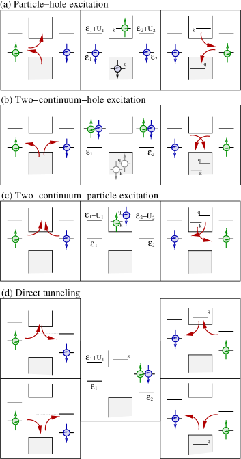
Figure 2: Several virtual tunnel processes contribute to the spin-spin interaction between the dots. These processes can be classified by the intermediate state of the system. While particle-hole excitation (a) leads to an RKKY-like interaction, the processes (b)-(d) are usually summarized as superexchange.

The second and third contributiosn to the spin-spin interaction originate from virtual two-particle(hole) excitations in the continuum Fermi sea, see Fig. 2(b) and (c). Two electrons tunnel coherently from or to the quantum dots. Thus, as intermediate virtual states, the two quantum dots are both doubly occupied (empty). Afterwards, the electrons tunneling crosswise back, interchanging the spins of the quantum dots. This process leads to the interactions $J_{2}$ and $J_{3}$.

Finally, the last contribution $J_{4}$ is caused by the possibility of a direct tunneling of one dot electron to the other dot. The virtual intermediate state is therefore one double occupied dot and one empty dot. The tunneling can happen through filled as well as empty states in the electron gas, see Fig. 2(d)

II.3 Relation to Coqblin-Schrieffer Model

In Ref. Coqblin1969, Coqblin and Schrieffer presented their widely used approach Schlottmann2000 ; Coleman1986 ; Bazhanov2003 ; Yang2005 to the two-impurity Anderson model. They performed a single Schrieffer-Wolff transformation, and project the resulting Hamiltonian of the single-occupied impurities. With this, they transform the two individual Anderson models into two individual s-d models or Kondo impurities. The spin of one quantum dot ${\bm{S}}_{i}$ is coupled to the bath electron spins by

$$H_{\rm Kondo}=\sum_{kq,\sigma\sigma^{\prime}}J^{i}_{kq}{\bm{S}}_{i}\cdot\,c^{\dagger}_{k\sigma}{\bm{\sigma}}_{\sigma\sigma^{\prime}}c_{q\sigma^{\prime}}\,,$$ (10)

see Appendix A for details. By treating that Hamiltonian in second order perturbation theory, they compute a RKKY-like spin-spin interactionRKKY of the form

$$\sum_{kq}J^{1}_{kq}J^{2}_{qk}\frac{n_{k}-n_{q}}{\varepsilon_{k}-\varepsilon_{q}}{\bm{S}}_{1}\cdot{\bm{S}}_{2}.$$ (11)

Even though Eq. (11) captures the basic features of Eq. (6), it is an expansion inconsistent in the order of the tunnel amplitudes. First, the initial Schrieffer-Wolff transformation generates not only terms of second order, but also the term $[iS_{1},[iS_{1},[iS_{1},H_{T}]$ which contributes in fourth order,Castro1995 see Eq. (4). Actually contributions from this higher-order term cancel several parts in Eq. (11), leading to Eq. (6). By truncating the transformation at second order, these contributions to the spin interaction are lost.

Second, the initial Schrieffer-Wolff transformation does not only generate the Kondo-Hamiltonian, but also terms in second order of the form $a_{1}^{\dagger}a_{2}$, which describe direct tunneling between the two quantum dots.BookMahan In a subsequent second order perturbation theory, these terms also lead to a inter-dot spin interaction. In Ref. Coqblin1969, these interactions are neglected due to the premature projection of the result of the Schrieffer-Wolff transformation on the single occupied dot subspace.

Interestingly, in the limit of energy levels far away from the Fermi energy, i.e., when one assumes that the spin coupling $J^{i}_{kq}$ approaches a constant, the Coqblin-Schrieffer approach generates the correct result. However, nowadays the Anderson model is extensively used to describe quantum dots.Durganandini2006 ; Tamura2004 ; Yang2005 In contrast to rare earth compounds or true atomic systems, the typical energy scale of the quantum dot level spectrum is several orders of magnitude smaller. Therefore in these artificial systems the application of the Coqblin-Schrieffer model needs to be handled with care.

II.4 Relation to fourth order perturbation theory

Starting from the two-impurity Anderson model, one can also derive a fourth order dot spin-spin interaction by perturbation theory,Zhang1986 ; Proetto1981 ; Proetto1982 ; Grewe1981 ; Kuramoto1981 ; Hewson1977 with or without diagrammatical help. The perturbation approach nearly reproduces our results Eq. (6)-(9) with one exception: the structure of the Fermi functions. Via perturbation theory one would expect for example that the two-lead-particle excitation, see Fig. 2(c), only happens if the two electron gas states $k$ and $q$ are empty, therefore the spin coupling $J_{2}$ should be proportional to $(1-n_{k})(1-n_{q})$. In contrast, the contribution from a Schrieffer-Wolff transformation is proportional to $(1-n_{q})$, and independent of $n_{k}$. By counting the operator commutators, one can directly determine that the spin-spin coupling derived by a two-stage Schrieffer-Wolff transformation can not generate terms, which contain four lead operators, which would be necessary for a product term like $n_{k}n_{q}$. The reason for this discrepancy between fourth order perturbation theory and Schrieffer-Wolff transformation lies in the procedure of integrating out the lead degrees of freedom, i.e., by the replacement of the thermal average of lead operators $\langle c^{{\dagger}}_{k}c_{k}\rangle_{\rm{th}}$ by the Fermi function $n_{k}$. In the case of the perturbation theory, the operators $c^{{\dagger}}_{k},c_{k}$ refer to the bare unperturbed electronic states of the lead, i.e., one assumes, that the lead is actually not perturbed by tunneling. After the Schrieffer-Wolff transformation, the lead operators refer to new lead states, which are hybridized with the localized dot states. By performing the thermal average, one therefore assumes that these new hybridized lead states are in thermal equilibrium, not the bare lead states. Therefore, it is not surprising that the results of a Schrieffer-Wolff transformation and perturbation theory differ. However, it is surprising that one can express the result of the Schrieffer-Wolff transformation in the same functional form one would expect from perturbation theory, except for the Fermi functions. Only due to this structure of terms one actually can, in the spirit of Feynman diagrams, assign virtual processes as shown in Fig. 2. For this reason, the grouping of terms in Eq. (6)-(9) is physically plausible but to some extent arbitrary. It has already been observed by Ruderman and KittelRKKY that by assuming certain symmetries of the tunnel amplitudes, the Pauli exclusion principle can actually become in part unimportant.

III Application to graphene nanoribbon quantum dots

Up to now, the computed result in Eq. (6-9) is general for the spin coupling of two qubits by a common continuum of states labeled by the indeces $k$ and $q$. In the following, we specify this continuum to the electronic structure of a graphene nanoribbon aligned along the $y$-direction.

III.1 Band structure

Bulk graphene has two independent Fermi points at the momenta $\bm{K}$ and $\bm{K}^{\prime}$ in reciprocal space, generating the valley degeneracy. Due to the armchair boundary conditions of the ribbon, the propagating wave states with momentum $\bm{K}+\bm{k}$ and $\bm{K}^{\prime}+\bm{k}$ are coupled.Brey2006 ; Brey2007 The confinement in x-direction leads to a further quantization of the transverse wave vector $k_{x}\equiv k_{n}=(n\pm 1/3)\pi/W$ with $W$ denoting the ribbon’s width and $n\in\mathbb{N}$. Therefore the continuum states can be characterized by the subband index $n$ and the momentum component $k_{y}\equiv k$ along the ribbon. Close to the Fermi energy, the dispersion relations becomes

$$\varepsilon_{k,n}=\hbar v_{F}\sqrt{k^{2}+k_{n}^{2}},$$ (12)

with the Fermi velocity $v_{F}$ of graphene. This dispersion resembles the dispersion of a massive relativistic particle.

The transverse confinement determines the energy gap $2\varepsilon_{g}=2\hbar v_{F}k_{0}$, which scales inversely with the ribbon width.Han2007 Due to this gap, electrons can be confined by electrostatic gates, in analogy to conventional semiconductors.Trauzettel2007 We assume the applied electric potential to be independent of the x-coordinate (see Fig. 1), therefore the band index $n$ is conserved. Therfore we only need to consider the continuum subband with the same band index as the bound state(s). Even if this symmetry is broken, the generalization to multi-subbands is straight forward.Shenoy2005 As a further simplification, we assume that by applying electrostatic gates, the dispersion relation of the extended states is still described by Eq. (12).

III.2 Tunnel amplitudes

The spin exchange is proportional to the product of the four tunnel amplitudes $t^{\star}_{1,k}(\bm{r}_{1})t_{2,k}(\bm{r}_{2})t_{1,q}(\bm{r}_{1})t^{\star}_{2,q}(\bm{r}_{2})$. In analogy to most cases studied in literature, we assume that the amplitude of the overlap of the bound states and the extended states does not explicitely depend on the momentum $k$ of the extended states. This assumption is valid if the wave function of the bound state is localized on a length scale smaller than the wave length of the extended state. In this case, one can approximate the localized wave function as a delta-function. However, in quantum dots in semiconductors in general, and in particular in the vicinity of a band edge, this assumption may not be valid. As $k$-independent tunnel amplitudes lead to a shorter spin exchange range, the spin exchange range derived in the following can be seen only as lower bound. Although the magnitude of the tunnel amplitude does not depend on $k$ within this approximation, the fact that the two quantum dots are separated in space gives rise to a relative phase. While in ordinary isotropic metals this phase is simply given by $e^{i\bm{k}\cdot\bm{r}_{i}}$, in graphene the valley degeneracy has to be taken into account. In nanoribbons, the energy eigenstates are phase-locked superposition of states of both valleys. Therefore, the overlap of the wave functionsTrauzettel2007 ; Brey2007 leads to a tunnel amplitude of the form

$$t_{1,k}(\bm{r}_{1})=t_{1}e^{-i\bm{k}\cdot\bm{r}_{1}}\frac{e^{-i\bm{K}\cdot\bm{r}_{1}}+e^{-i\bm{K}^{\prime}\cdot\bm{r}_{1}}}{\sqrt{2}}.$$ (13)

The spin coupling therefore will always contain a contribution which oscillates on inter-atomic distances, and one contribution, which varies on the length scale of the envelope wave function. As the quantum dots under consideration are not spatially defined with lattice site precision, we expect that the oscillating contribution to the spin exchange will average out.

III.3 Spin-exchange range

Which of the virtual tunnel process (see Fig. 2) dominates the spin exchange between two quantum dots depends on the alignment of the dot energy levels, band gap, and edges. Roughly speaking, the virtual process requiring the lowest excitation energy will dominate. As we assume the graphene nanoribbon to be nearly undoped, the Fermi energy of the system lies within the band gap. Therefore the valence band is entirely filled, and the conduction band is empty. The RKKY-like exchange interaction via a particle-hole excitation in the continuum will be suppressed by the band gap $2\varepsilon_{g}$, and superexchange processes will dominate. In the following, we will discuss the scenario shown in Fig. 3, where the quantum dot level lies close to the valence band, and the charging energy is smaller than the band gap.

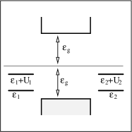
Figure 3: If the quantum dot level lies close to the valence band, and the charging energy is smaller than the band gap, direct tunneling processes will dominate the spin exchange between the quantum dots.

In this level alignment, direct tunneling processes via the valence band dominate the spin exchange. The resulting integrals can be computed by Cauchy’s integral formula. The exchange due to direct tunneling turns out to be

$$J = -\frac{|t_{1}|^{2}|t_{2}|^{2}}{4\Delta E^{2}}\frac{1}{\varepsilon_{2}+U_{2}-\varepsilon_{1}}\frac{(\varepsilon_{2}+U_{2})^{2}}{\varepsilon_{g}^{2}-(\varepsilon_{2}-U_{2})^{2}}$$ (14)

$$\times e^{-2\frac{\sqrt{\varepsilon_{g}^{2}-(\varepsilon_{2}+U_{2})^{2}}}{\hbar v_{F}}\Delta r}+(1\leftrightarrow 2)$$

with the quantum dot distance $\Delta r=|\bm{r}_{1}-\bm{r}_{2}|$. The energy $\Delta E=\hbar v_{F}/L$ is the energy splitting of the continuum states, with $L$ being the length of the ribbon. As the tunnel amplitudes $t_{i}$ decrease with the real space particle density of the band states with $1/\sqrt{L}$, the strength of the spin exchange is independent of the overall length of the ribbon.

The strength of the spin coupling driven by direct tunneling diverges within $4^{th}$ order, if the single occupied state of one dot becomes resonant with the double occupied state of the other dot. The range $\lambda=\hbar v_{F}/2\sqrt{\varepsilon_{g}^{2}-(\varepsilon_{2}+U_{2})^{2}}$ of the coupling Eq. (14) on the other side is controlled by the energy separation between the double occupied state of the one dot, and the valence band edge at energy $-\varepsilon_{g}$. If one assumes, that the single occupied states of the two dots are close to the band edge ($\varepsilon_{g}\approx\varepsilon_{i}$), the exchange range scales as $\hbar v_{F}/\sqrt{8\varepsilon_{g}U_{i}}$. For a graphene nanoribbon with width of $50\,\mathrm{nm}$ and a quantum dot with a charging energy of $4\,\mathrm{meV}$,Stampfer2008 this length is of order $50\,\mathrm{nm}$, i.e. comparable to the quantum dot length.

If one assumes that, in analogy to a capacitor, the charging energy of a quantum dot scales inversely with its area,Stampfer2008 then the range of the spin exchange interaction scales linearly with the width of the nanoribbon.

III.4 Further considerations

The lower bound for the spin exchange range between quantum dots in a graphene nanoribbon is given by the ribbon width. For this result we considered only virtual tunnel processes via free continuum states. In addition, also direct tunneling between the quantum dot states can occur. If the quantum dot level approaches the band gap, the bound electron leaks further and further into the barrier due to the weakening of the confinement. Therefore it can happen that two neighboring quantum dot wave functions can acquire a non-vanishing overlap, and direct tunneling becomes possible. Direct tunneling is accompanied also by a spin-exchange interaction.Trauzettel2007

Furthermore, we assumed so far that the graphene nanoribbon is infinitely long. This assumption is hidden in the approach to treat the continuum states with momentum $k$ independent on the state $-k$. However, if a finite ribbon length leads to a defined phase relation of the forward and backward propagating states, then one part of the tunnel amplitude will become entirely independent on the momentum $k$, and therefore on the distance $\Delta\bm{r}$.Trauzettel2007 (cf. also the discussion of section III.2.) If this case, the range $\lambda$ of the spin exchange is not determined by the dephasing of the exchange contributions of different states within the Fermi sea, but only on the phase coherence length of the extended states.

IV Conclusions

In this paper, we discussed the spin exchange between localized states which are only indirectly coupled via a continuum of states. Using a 2-stage Schrieffer-Wolff transformation, we transformed a 2-impurity Anderson model into an effective spin Hamiltonian. Based on our result, we discussed the validity of the Coqblin-Schrieffer approach to this problem. Furthermore, by a re-ordering the terms, we were able to directly compare the Schrieffer-Wolff result to perturbation theory, and observe distinct differences that originate from different assumptions on the continuum of states.

As an application of the formalism developed here, we discussed the spin exchange interaction between electrostatically confined quantum dots in a graphene nanoribbon, as shown in Eq. (14). As a lower bound, we derive a range of this spin exchange of the order of the nanoribbon width. However, the dot energies can be adjusted in such a way as to extend the exchange coupling to longer distances.

Appendix A First Schrieffer-Wolff Transformation

The generator of the first Schrieffer-Wolff transformation must fullfill the relation $[iS_{1},H_{0}]=-H_{T}$. As the part of the Hamiltonian $H_{0}$ only contain number operators, i.e., is quadratic or quartic in the fermion operators, one can deduce, that $iS$ must have the same structure as the tunnel Hamiltonian $H_{T}$, up to a prefactor containing either constants or number operators. With such an ansatz, the generator of the first Schrieffer-Wolff transformation is found to be

$$iS_{1}=$$ (15)

$$\sum_{i,k,\sigma}\frac{t_{i,k}}{\varepsilon_{k}-\varepsilon_{i}-U_{i}n_{i\bar{\sigma}}}c^{\dagger}_{k\sigma}a_{i\sigma}-\frac{t^{\star}_{i,k}}{\varepsilon_{k}-\varepsilon_{i}-U_{i}n_{i\bar{\sigma}}}a^{\dagger}_{i\sigma}c_{k\sigma}\qquad$$

$$=\sum_{i,k,\sigma}t_{i,k}\left[\frac{1-n_{i\bar{\sigma}}}{\varepsilon_{k}-\varepsilon_{i}}+\frac{n_{i\bar{\sigma}}}{\varepsilon_{k}-\varepsilon_{i}-U_{i}n_{i\bar{\sigma}}}\right]c^{\dagger}_{k\sigma}a_{i\sigma}-{\rm h.c.}$$

This transformation removes the interaction term of first order in the tunneling amplitude, but instead generates higher order interactions starting in second order of $t$. The new interaction Hamiltonian $H_{T}^{(1)}=\frac{1}{2}[iS_{1},H_{T}]+O(t^{3})$ becomes

$$H_{T}^{(1)} = \sum_{i,kq,\sigma}J^{i}_{kq}{\bm{S}}_{i}\cdot{\bm{s}}_{kq}$$

$$+ \frac{-1}{2}\sum_{ij,k,\sigma}A^{k}_{ij}a^{{\dagger}}_{i\sigma}a_{j\sigma}$$

$$+$$ dot double empty/filling terms

$$+$$ spin independent lead scattering-terms

The first term resembles the Kondo model. The spin of the quantum dot ${\bm{S}}_{i}=\sum_{\sigma\sigma^{\prime}}a^{\dagger}_{i\sigma}\,{\bm{\sigma}}_{\sigma\sigma^{\prime}}\,a_{i\sigma^{\prime}}$ couples to the band spin ${\bm{s}}_{kq}=\sum_{\sigma\sigma^{\prime}}c^{\dagger}_{k\sigma}\,{\bm{\sigma}}_{\sigma\sigma^{\prime}}\,c_{q\sigma^{\prime}}$. The coupling strength is given by $J^{i}_{kq}=t^{\star}_{i,q}t_{i,k}\left[\frac{1}{\varepsilon_{k}-\varepsilon_{i}}-\frac{1}{\varepsilon_{k}-\varepsilon_{1}-U_{1}}+\frac{1}{\varepsilon_{q}-\varepsilon_{i}}-\frac{1}{\varepsilon_{q}-\varepsilon_{1}-U_{1}}\right]$. The second term describes a direct tunneling of one quantum-dot electron to another dot with the effective coupling strength $A^{k}_{ij}=t^{\star}_{i,k}t_{j,k}\left[\frac{1-n_{i\bar{\sigma}}}{\varepsilon_{k}-\varepsilon_{i}}+\frac{n_{i\bar{\sigma}}}{\varepsilon_{k}-\varepsilon_{i}-U_{i}}+\frac{1-n_{j\bar{\sigma}}}{\varepsilon_{k}-\varepsilon_{j}}+\frac{n_{j\bar{\sigma}}}{\varepsilon_{k}-\varepsilon_{j}-U_{j}}\right]$ with $\bar{\sigma}$ denoting the opposite spin orientation of $\sigma$. This term can also lead to a spin exchange in fourth order, so it is not negligible. The further parts of Eq. (A) include processes, which change the occupation of one quantum dot by two electrons, and spin-independent scattering of continuum electrons at one dot.

Appendix B Second Schrieffer-Wolff Transformation

For the second Schrieffer-Wolff Transformation, the procedure is very similar. Using the ansatz for $iS_{2}$ that resembles the second order part of the interaction term, derived by the first transformation. However, as one is in the end interested in the fourth-order parts of the Hamiltonian, which couple two quantum dot spins and conserve the quantum dot occupation number, one only needs to consider the first two parts of Eq. (A). The generator for the transformation therefore can be written as $iS_{2}=iS_{2}^{(a)}+iS_{2}^{(b)}$ with

$$iS_{2}^{(a)} = \sum_{i,kq,\sigma}\frac{1}{\varepsilon_{k}-\varepsilon_{q}}J^{i}_{kq}{\bm{S}}_{i}\cdot{\bm{s}}_{kq}$$ (17)

$$iS_{2}^{(b)} = \frac{-1}{2}\sum_{ij,k,\sigma}\frac{1}{\varepsilon_{i}+U_{i}n_{i\bar{\sigma}}-\varepsilon_{j}-U_{j}n_{j\bar{\sigma}}}A^{k}_{ij}a^{\dagger}_{i\sigma}a_{j\sigma}$$

The other second order terms finally drop out in the end, when the Hamiltonian is projected on the subspace of single occupied quantum dots. For the regrouping of terms in Eq. (5-9), one needs the symmetry of the expressions under the replacement $1\leftrightarrow 2$ and $k\leftrightarrow q$.

References

- (1) D. Loss and D. P. DiVincenzo, Phys. Rev. A 57, 120 (1998).
- (2) R. Hanson, L. P. Kouwenhoven, J. R. Petta, S. Tarucha, and L. M. K. Vandersypen, Rev. Mod. Phys. 79, 1217 (2007).
- (3) K.S. Novoselov, A.K. Geim, S.V. Morozov, D. Jiang, Y. Zhang, S.V. Dubonos, I.V. Grigorieva, and A.A. Firsov, Science 306, 666 (2004).
- (4) K.S. Novoselov, A.K. Geim, S.V. Morozov, D. Jiang, M.I. Katsnelson, I.V. Grigorieva, S.V. Dubonos, and A.A. Firsov, Nature 438, 197 (2005).
- (5) Y. Zhang, Y.-W. Tan, H.L. Stormer, and P. Kim, Nature 438, 201 (2005).
- (6) A.K. Geim and K.S. Novoselov, Nature Mater. 6, 183 (2007).
- (7) M.I. Katsnelson, Mater. Today 10, 20 (2007).
- (8) B. Trauzettel, D. V. Bulaev, D. Loss, and G. Burkard, Nature Physics 3, 192 (2007), cond-mat/0611252.
- (9) N. Tombros, C. Jozsa, M. Popinciuc, H. T. Jonkman, B. J. van Wees, Nature 448, 571-574 (2007).
- (10) S. Sahoo, T. Kontos, J. Furer, C. Hoffmann, Matthias Gräber, A. Cottet and C. Schönenberger, Nature Physics 1, 99 (2005).
- (11) V. B. Shenoy, Phys. Rev. B 71, 125431 (2005).
- (12) M.I. Katsnelson, K.S. Novoselov, and A.K. Geim, Nature Phys. 2, 620 (2006).
- (13) O. Klein, Z. Phys. 53 157 (1929).
- (14) C. Stampfer, J. Güttinger, F. Molitor, D. Graf, T. Ihn, and K. Ensslin, Appl. Phys. Lett. 92, 012102 (2008).
- (15) P. G. Silvestrov and K. B. Efetov, Phys. Rev. Lett. 98, 016802 (2007).
- (16) L. Brey and H. A. Fertig, Phys. Rev. B 73, 235411 (2006).
- (17) M. Y. Han, B. Oezyilmaz, Y. Zhang, and P. Kim, Phys. Rev. Lett, 98, 206805 (2007).
- (18) M. A. Ruderman and C. Kittel, Phys. Rev. 96, 99 (1954); T. Kasuya, Prog. Theor. Phys. 16, 45 (1956); K. Yosida, Phys. Rev. 106, 893 (1957); J. H. Van Vleck, Reviews of Modern Physics 34, 681-686 (1962).
- (19) K. W. -K. Shung, Phys. Rev. B 34, 979 (1986).
- (20) G. Bastard and C. Lewiner, Phys. Rev. B 20, 4256 (1979).
- (21) B. Wunsch, T. Stauber, F. Sols, and F. Guinea, New Journal of Physics 8 (12), 318 (2006).
- (22) S. Saremi, Phys. Rev. B 76, 184430 (2007).
- (23) E. H. Hwang and S. Das Sarma, Phys. Rev. Lett. 101, 156802 (2008).
- (24) V. K. Dugaev, V. I. Litvinov, and J. Barnas, Phys. Rev. B 74, 224438 (2006).
- (25) T. Ando, J. Phys. Soc. Japan 75, 074716 (2006).
- (26) D. N. Aristov, Phys. Rev. B 55, 8064 - 8066 (1997).
- (27) V. I. Litvinov and V. K. Dugaev, Phys. Rev. B 58, 3584 - 3585 (1998).
- (28) T. Balcerzak, JMMM 310, 1651 (2007).
- (29) Z. Ba̧k, Solid State Communications, 118, 43 (2001)
- (30) P. Durganandini, Phys. Rev. B, 74, 155309 (2006)
- (31) C. H. Ziener, S. Glutsch, and F. Bechstedt, Phys. Rev. B 70, 075205 (2004).
- (32) E. Bauer, J. Advances in Physics 40, 417 (1991).
- (33) P. Schlottmann, Phys. Rev. B 62, 10067 (2000).
- (34) C. Proetto and A. López, Phys. Rev. B 25, 7037 (1982).
- (35) A. C. Hewson, J. Phys. C: Solid State Phys. 10 4973 (1977).
- (36) J. C. Mohanty, P. K. Misra and S. D. Mahanti, J. Phys. C: Solid State Phys. 14 L1125 (1981).
- (37) B. Alascio, A. López and C. F. E. Olmedo, J. Phys. F: Met. Phys. 3 1324 (1973).
- (38) G. D. Mahan, Many particle physics, Plenum Press, New York (1991)
- (39) P. Coleman, Lectures on the Physics of Highly Correlated Electron Systems VI, Editor F. Mancini, American Institute of Physics, New York (2002), p.79 - 160; cond-mat/0206003.
- (40) C. Proetto, A. Lopez, Phys. Rev. B 24, 3031 - 3036 (1981).
- (41) A. Singh, A. Datta, S. K. Das, and V. A. Singh, Phys. Rev. B 68, 235208 (2003).
- (42) J. Zaanen and A. M. Oleś, Phys. Rev. B 37, 9423 (1988).
- (43) D. Ihle and M. Kasner, Phys. Rev. B 42, 4760 (1990).
- (44) Kh. Eid, M. Matlak, J. Zieliski, physica status solidi (b), 187, 589 (1995).
- (45) L. C. Andreani and H. Beck, Phys. Rev. B 48, 7322 - 7337 (1993)
- (46) J. Simonin, arXiv:cond-mat/0703531;J. Simonin, arXiv:cond-mat/0607620; J. Simonin, Phys. Rev. B 73, 155102 (2006); J. Simonin, cond-mat/0510580.
- (47) N. Grewe and H. Keiter, Phys. Rev. B 24, 4420 (1981).
- (48) Y. Kuramoto, Z. Phys. B 40, 293 (1981).
- (49) N. E. Bickers, Rev. Mod. Phys. 59, 845 (1987).
- (50) V. V. Bazhanov, S. L. Lukyanov, and A. M. Tsvelik, Phys. Rev. B 68, 094427 (2003).
- (51) E. Kolley, W. Kolley, and R. Tietz, phys. stat. sol. (B), 204, 763 (1997).
- (52) E. Kolley, W. Kolley and R Tietz, J. Phys.: Condens. Matter 10, 657 (1998).
- (53) E. Kolley, W. Kolley and R. Tietz, J. Phys.: Condens. Matter 4, 3517 (1992).
- (54) T. Minh-Tien, Physica C: Superconductivity 223, 361 (1994).
- (55) T. Tzen Ong and B. A. Jones, arXiv:cond-mat/0602223
- (56) B. Coqblin and J. R. Schrieffer, Phys. Rev. 185, 847 (1969).
- (57) Y.F. Yang and K. Held, Phys. Rev. B 72, 235308 (2005)
- (58) C. Sanchez-Castro, B. R. Cooper, and K. S. Bedell, Phys. Rev. B 51, 12506 (1995).
- (59) B. Cornut and B. Coqblin, Phys. Rev. B 5, 4541 (1972).
- (60) R. Siemann and B. R. Cooper, Phys. Rev. Lett. 44, 1015 (1980).
- (61) H. Tamura, K. Shiraish, and H. Takayanagi, Jpn. J. Appl. Phys. 43, L691 (2004).
- (62) J. R. Schrieffer and P. A. Wolff, Phys. Rev. 149, 491 (1966).
- (63) H. Bruus and K. Flensberg, Many-Body Quantum Theory in Condensed Matter Physics: An Introduction, Oxford University Press, Oxford (2004).
- (64) A. C. Hewson, The Kondo Problem to Heavy Fermions, Cambridge University Press, Cambridge (2003).
- (65) One could be temped to assume, that the sepatration of the interaction terms in Eq. (4) resembles the distinction of different types of physical interactions. This qppears not to be the case.
- (66) P. Coleman and N. Andrei, J. Phys. C: Solid State Phys. 19 3211 (1986).
- (67) Q. Zhang and P. M. Levy, Phys. Rev. B 34, 1884 (1986)
- (68) L. Brey and H. A. Fertig, Phys. Rev. B 75, 125434 (2007).