Markov chain Monte Carlo estimation of default and recovery: dependent via the latent systematic factor

Abstract

It is a well known fact that recovery rates tend to go down when the number of defaults goes up in economic downturns. We demonstrate how the loss given default model with the default and recovery dependent via the latent systematic risk factor can be estimated using Bayesian inference methodology and Markov chain Monte Carlo method. This approach is very convenient for joint estimation of all model parameters and latent systematic factors. Moreover, all relevant uncertainties are easily quantified. Typically available data are annual averages of defaults and recoveries and thus the datasets are small and parameter uncertainty is significant. In this case Bayesian approach is superior to the maximum likelihood method that relies on a large sample limit Gaussian approximation for the parameter uncertainty. As an example, we consider a homogeneous portfolio with one latent factor. However, the approach can be easily extended to deal with non-homogenous portfolios and several latent factors.

Keywords: parameter uncertainty, probability of default, loss given default, economic capital, Markov chain Monte Carlo, Bayesian inference, credit risk

¹ CSIRO Mathematics, Informatics and Statistics, Sydney, Australia; e-mail: Xiaolin.Luo@csiro.au
² CSIRO Mathematics, Informatics and Statistics, Sydney, Australia; e-mail: Pavel.Shevchenko@csiro.au
^∗ Corresponding author

1 Introduction

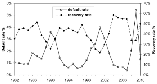
Figure 1: Global corporate default and recovery annual rates from Moody’s (2011)

Default and recovery rates are key components of Loss Given Default (LGD) credit risk models. The classic LGD model implicitly assumes that the default rates and recovery rates are independent (Bluhm et al 2002). There is empirical evidence that recovery rates tend to go down just when the number of defaults goes up in economic downturns that is clearly observed in historical data in Figure 1. Motivated by this fact, Frye (2000a), Pykhtin (2003) and Düllmann and Trapp (2004) extended the classic model to include systematic risk in recovery rates, incorporating a non-zero correlation between default rates and recovery rates driven by the systematic factor. They considered three extensions to account for the systematic risk in recovery rates under three different assumptions for the distribution of recovery rates: Frye (2000a) – a normal distribution; Pykhtin (2003) – a log-normal distribution; Düllmann and Trapp (2004) and Schönbucher (2001) – a logit-normal distribution. The extended models are still parsimonious, yet they represent an important enhancement of credit risk models used in earlier practice, for example, CreditMetrics (Gupton et al 1997) and CreditRisk+ (Credit Suisse Financial Products 1997) that do not account for systematic risk factor driving both default and recovery rates. Other extensions considering the correlation between risk drivers of default and recovery are found in Cantor and Varma (2005) and Rösch and Scheule (2005). These models (among others) have been suggested by some banks for assessment of the Basel II “downturn LGD” requirement, see Basel Committee on Banking Supervision (2005). The Basel II “downturn LGD” reasoning is that recovery rates may be lower during economic downturns when default rates are high; and that a capital should be sufficient to cover losses during these adverse circumstances. For a good review of credit risk LGD models, see Altman (2006).

Düllmann and Trapp (2004) summarized the empirical literature on systematic risk in recovery rates, and found a broad agreement that default rates and business cycle are correlated. They calculated the maximum likelihood estimators (MLEs) of model parameters for the default and recovery rate distributions; estimated the correlations of default and recovery rates with the systematic risk factor; and found that economic capital (EC), defined as the 0.999 quantile of the annual loss distribution, is significantly higher in the extended LGD models (in comparison with the classic one-factor model) due to dependence of recoveries on the systematic risk factor. It was also observed that EC estimates are very close to each other for all three distributional assumptions for the recovery rates.

Publicly available data provided by Moody’s or Standard&Poor’s rating agencies are annual averages of defaults and recoveries. These data are of limited size, covering a couple of decades at most. For example, in the study of Düllmann and Trapp (2004), the default and recovery data have eighteen points covering an eighteen-year period 1982-1999. Inevitably the limited data size could pose significant instability and uncertainty in the LGD model parameter estimates. None of the various studies, including the extension work of Frye (2000a, 2000b), Pykhtin (2003) and Düllmann and Trapp (2004) specifically addressed the quantitative impact of parameter uncertainty. Increasingly, quantification of parameter uncertainty has become a key component of financial risk modeling and management. Recent examples of addressing parameter uncertainty in operational risk and insurance include Luo et al (2007) and Peters et al (2009a).

Bayesian inference is a convenient approach to jointly estimate all model parameters and latent factors, and all relevant uncertainties. It is especially useful when data are limited and parameter uncertainty is large. In this case Bayesian approach is superior to the maximum likelihood method that relies on a large sample limit Gaussian approximation for the parameter uncertainty. Under the Bayesian approach, the inference is based on the distribution of the parameters and latent factors given data (so-called posterior distribution). Typically, the posterior distribution is not available in closed-form but can be easily estimated numerically using Markov chain Monte Carlo (MCMC) method. In this paper, we demonstrate how the extended LGD model can be estimated using Bayesian inference and MCMC method. For illustration, we consider homogeneous portfolio with one latent factor. However, the approach can be easily extended to non-homogeneous portfolios and several latent factors.

The organization of this paper is as follows. Section 2 first describes the credit risk model setup, particularly the extended default and recovery models considered by Frye (2000a), Pykhtin (2003) and Düllmann and Trapp (2004). This is followed by a discussion on various EC estimates and the corresponding algorithms, both for the finite number of borrowers and for the limiting case of the infinitely granular portfolio. The emphasis is on how to account for parameter uncertainty using Bayesian inference and MCMC. Section 3 presents the likelihood functions for the LGD model. This includes the full joint likelihood for default and recovery as well as two-stage approximation used in Frye (2000b) and Düllmann and Trapp (2004). For the latter, we derive the closed-form MLEs for the recovery process parameters in addition to the known closed-form MLEs for the default parameters. Section 4 describes the Bayesian inference formulation and the MCMC simulation algorithm for the posterior distribution of the LGD model parameters. Sections 5 and 6 present MCMC results in comparison with the MLEs using annual default and recovery rates for corporate bonds. Results in Section 5 are for the 1982-1999 data period, the same time period as studied in Düllmann and Trapp (2004), while results in Section 6 are for the period 1982-2010 covering the recent global financial crisis. Concluding remarks are given in the final section.

2 LGD Model

The standard one-factor LGD model assumes a homogenous loan portfolio where the distribution of its loss vector that collects losses of individual loans is exchangeable (invariant) under permutations of its components. Following Frye (2000a), Pykhtin (2003) and Düllmann and Trapp (2004), the key characteristics of the one-factor model are summarized as follows.

Consider a portfolio of $J$ borrowers (firms) over a chosen time horizon. To avoid cumbersome notation, we assume that the $j$th borrower has one loan with principal amount $A_{j}$. The loss rate (loss amount relative to the loan amount) of the portfolio due to defaults is

$$L=\sum_{j=1}^{J}w_{j}L_{j}=\sum_{j=1}^{J}w_{j}I_{j}\max(1-R_{j},0),$$ (1)

where we have the following definitions.

• $w_{j}$ is the weight of loan $j$ in the portfolio, $w_{j}=A_{j}/\sum_{m=1}^{J}A_{m}$.

• $L_{j}$ is the loss rate of loan $j$ due to potential default.

• $1-\max(1-R_{j},0)=\min(R_{j},1)$ is the recovery rate of loan $j$ after default.

• $I_{j}$ is an indicator variable associated with the default of firm $j$, $I_{j}=1$ if firm $j$ defaults, otherwise $I_{j}=0$.

Quantity $R_{j}$ can be loosely interpreted as the value of collateral per unit of exposure (e.g. see Frye 2000a). When this quantity exceeds 1 (i.e. the value of collateral exceeds the value of exposure), then $100\%$ recovery is assumed. In general $R_{j}$ is not the same as recovery rate since the latter is subject to a cap of 1.

Following Düllmann and Trapp (2004), in this study we do not explicitly impose the restriction $0\leq R_{j}\leq 1$. In fact, results in Düllmann and Trapp (2004) show that the unbounded normal distribution for recovery rate gives a capital estimate very close to that given by the properly bounded logit-normal distribution (the relative difference is less than $1\%$). As in Düllmann and Trapp (2004), for simplicity the term “recovery rate” is used for the quantity $R_{j}$ in the rest of the paper.

Remark: The above notation is for a given time period. Later, starting from Section 3, we consider the model over a number of time periods $t=1,2,\ldots,T,T+1$ that will add index $t$ to all random variables. Here, $T+1$ refers to the next year. It is assumed that all random variables involved in the model are independent between different time periods. However, the model can be easily extended to have explicit time dependence.

2.1 Modeling Default

Denote the probability of default for firm $j$ by $p$, i.e. $\mathrm{Pr}[I_{j}=1]=p$. Let $C_{j}$ be an underlying latent random variable such that firm $j$ defaults if $C_{j}<\Phi^{-1}(p)$, where $\Phi(\cdot)$ is the standard normal distribution and $\Phi^{-1}(\cdot)$ is its inverse. That is, $I_{j}=1$ if $C_{j}<\Phi^{-1}(p)$ and $I_{j}=0$ otherwise. $C_{j}$ describes the overall financial condition (financial well-being) of firm $j$ over a time horizon. The value $C_{j}$ for each firm depends on a systematic risk factor $X$ and a firm specific (idiosyncratic) risk factor $Z^{C}_{j}$ as

$$C_{j}=\sqrt{\rho}X+\sqrt{1-\rho}Z^{C}_{j},$$ (2)

where $Z^{C}_{1},\ldots,Z^{C}_{J}$ are all independent. Also, $X$ and $Z^{C}_{j}$ are assumed to be independent and from the standard normal distribution.

Conditional on $X$, the financial conditions of any two firms are independent. The parameter $\rho$ quantifies the extent of exposure of a firm’s asset value to the fluctuations in the business cycle. Unconditionally, it measures the correlation between financial conditions of two firms. The value of $\rho\in[0,1]$ is assumed to be the same for all firms but can be extended to be firm specific if required.

2.2 Modeling Recovery

The extended LGD models proposed and studied by Düllmann and Trapp (2004), Frye (2000a, 2000b) and Pykhtin (2003) account for systematic risk in recovery rates under three different assumptions for the distribution of recovery rates. Define

$$V_{j}=\mu+\sigma\sqrt{\omega}X+\sigma\sqrt{1-\omega}Z_{j},\hskip 8.5359pt\omega\in[0,1],$$ (3)

where $X$ and $Z_{j}$ are assumed to be independent and from the standard normal distribution, and parameter $\omega$ is restricted to the interval $[0,1]$. Also, $Z_{j}$ and $Z_{j}^{C}$ are assumed independent too. Note, the one-factor model in Pykhtin (2003) allows for correlation between $Z_{j}$ and $Z_{j}^{C}$. The three models for the recovery rate are then defined through $V_{j}$ as follows.

• The first extended model, as initially suggested by Frye (2000a), assumes a normal distribution for the recovery rates, i.e. the recovery rate $R_{j}$ of loan $j$ is given by

  $$R_{j}=V_{j}.$$ (4)

  An advantage of the above model is that parameters $\mu$ and $\omega$ directly represent the mean and correlation of recoveries respectively.

• The second extension, initially proposed by Schönbucher (2001), assumes that the recovery rate $R_{j}$ follows a logit-normal distribution, i.e.

  $$R_{j}=\frac{\exp(V_{j})}{1+\exp(V_{j})}.$$ (5)

  The above model satisfies the restriction $0<R_{j}<1$.

• The third model, following Pykhtin (2003), has a log-normal distribution for the recovery rate

  $$R_{j}=\exp(V_{j}).$$ (6)

The study by Düllmann and Trapp (2004) shows that EC estimates from the above three recovery models are very close to each other; only about $2\%$ difference exists among the EC values estimated by these models. In addition, they carried out Shapiro-Wilk test and Jarque-Bera test for normality, and found that the normal distribution assumption for the recovery rate is favored by the p-values over the other two models. Thus in the present study, we will concentrate on the first recovery model given by (4), i.e. we assume a normal distribution for the recover rate, but it is not difficult to use other recovery distributions. Another reason for our choice of model (4) is because we do not have the original data for individual recoveries but only the average recovery rates; and we can use the fact that the distribution of the average of normally distributed independent random variables is still normal.

2.3 Economic Capital

Following the literature, we define the economic capital (EC) as the 0.999 quantile of the distribution of loss $L$ defined in (1). Specifically, the quantile $Q_{q}$ is defined as

$$Q_{q}({\bm{\theta}})\equiv Q_{q}=\inf\{z:\Pr[L>z|\bm{\theta}]\leq 1-q\}=\inf\{z:F_{L}(z|\bm{\theta})\geq q\},$$ (7)

where $q$ is a quantile level (e.g. 0.999); $F_{L}(z|\bm{\theta})$ is distribution function of the random loss $L$; the corresponding density of $L$ is denoted as $f_{L}(z|\bm{\theta})$; and ${\bm{\theta}}=(p,\rho,\mu,\sigma,\omega)$ are the model parameters.

There are different ways of estimating this high quantile, some are based on point estimates (e.g. MLEs) of parameters and others account for parameter uncertainty. We are interested in comparing these different estimates of the quantile and quantifying the impact of different assumptions, particularly the impact of parameter uncertainty.

2.3.1 Quantile point estimates

For a given model with parameters ${{\bm{\theta}}}$, the quantile $Q_{q}({\bm{\theta}})$ is a function of ${{\bm{\theta}}}$. Typically, given observations, the MLEs ${{\widehat{\bm{\theta}}}}$ are used as the “best fit” point estimates for ${{\bm{\theta}}}$. Then, the loss density for the next time period is estimated as $f_{L}(z|{{\widehat{\bm{\theta}}}})$ and its quantile is estimated as $Q_{q}({{\widehat{\bm{\theta}}}})$. In general, the distribution of $L$ is not tractable in closed form for an arbitrary portfolio. In this case, Monte Carlo method for simulating $L$ in (1) for given parameters ${\bm{\theta}}$ can be used as follows.

Algorithm 1 (Quantile given parameters)

1. Draw a single independent sample from the standard normal distribution for the systematic factor $X$.

2. For each borrower $(j=1,\ldots,J)$, draw an independent sample from the standard normal distribution for the idiosyncratic default risk factor $Z^{C}_{j}$; calculate $C_{j}$ as in (2); and let $I_{j}=1$ if $C_{j}<\Phi^{-1}(p)$ and $I_{j}=0$ otherwise.

3. Draw an independent sample from the standard normal distribution for the idiosyncratic recovery factor $Z_{j}$ and calculate $R_{j}=\mu+\sigma\sqrt{\omega}X+\sigma\sqrt{1-\omega}Z_{j}$.

4. Find loss $L$ for the entire portfolio using (1). This is a sample from the loss distribution $F_{L}(\cdot|\bm{\theta})$.

5. Repeat steps 1-4 to obtain $N$ samples of $L$ with $N$ sufficiently large for high quantile calculations (i.e. numerical error due to finite number of simulations is small enough).

6. Estimate $Q_{q}({\bm{\theta}})$ using obtained samples of $L$ in the standard way (e.g. using sample with the index $\lceil Nq\rceil$ after sorting in the ascending order).

In practice, the parameters ${{\bm{\theta}}}$ are unknown and it is important to account for this uncertainty when the quantile is estimated, especially in the case of small datasets. A standard frequentist approach to estimate this uncertainty is based on limiting results of normally distributed MLEs for large datasets. Then information matrix (calculated from the second order derivatives of the likelihood) is used to estimate the covariances between MLEs. In this paper we take Bayesian approach, because dataset is small and the distribution of parameter uncertainty is very different form normal. Estimation of the quantile accounting for parameter uncertainty under the Bayesian inference framework will be discussed in Section 4.

2.3.2 Economic capital under the limiting condition

In the case of a diversified portfolio with a large number of borrowers, the idiosyncratic risk can be eliminated and the loss depends on $X$ only. Gordy (2002) has shown that the distribution of portfolio loss $L$ has a limiting form as $J\rightarrow\infty$, provided that each weight $w_{j}$ goes to zero faster than $1/\sqrt{J}$. The limiting loss rate $L^{\infty}$ is given by the expected loss rate conditional on the systematic factor $X$

$$L^{\infty}\equiv L^{\infty}(X)=E[L|X]=\sum_{j=1}^{J}w_{j}E[L_{j}|X]=\sum_{j=1}^{J}w_{j}E[I_{j}\max(1-R_{j},0)|X],$$ (8)

i.e. the limiting loss $L^{\infty}$ is just a function of $X$ and the distribution of $L^{\infty}$ is fully implied by the distribution of $X$.

Conditional on $X$, the default indicator variable $I_{j}$ and the recovery rate $R_{j}$ are independent because $Z^{C}_{j}$ in (2) and $Z_{j}$ in (3) are independent. Thus, the limiting loss (8) for $J\rightarrow\infty$ becomes

$$L^{\infty}=\sum_{j=1}^{J}w_{j}E[I_{j}|X]E[\max(1-R_{j},0)|X]=\sum_{j=1}^{J}w_{j}\Lambda_{j}(X)S_{j}(X),$$ (9)

where $\Lambda_{j}(X)=E[I_{j}|X]$ is the conditional probability of default of firm $j$ and $S_{j}(X)=E[\max(1-R_{j},0)|X]$ is the conditional expected value of loss rate, both are functions of $X$.

Bank loans are subject to the borrower specific risk and systematic risk. The former can be controlled or even neutralized by diversification. Note that (8-9) is valid for a non-homogeneous portfolio. For a homogeneous portfolio, probability of default and recovery rates (or loss given default) are not firm specific, i.e. $\Lambda_{j}(X)=\Lambda(X)$ and $S_{j}(X)=S(X)$ for all $j$, and (9) simplifies to

$$L^{\infty}=\sum_{j=1}^{J}w_{j}\Lambda(X)S(X)=\Lambda(X)S(X)=L^{\infty}(X).$$ (10)

That is, the limiting loss rate of the diversified homogenous portfolio is a function of $X$ only. As in the model underlying the internal ratings-based risk weights of Basel II, EC is determined with the assumption that the bank loan portfolio is fully diversified and EC is only held for systematic credit risk. Because $L^{\infty}(X)$ is a monotonic decreasing function of random variable $X$, and $X$ is from the standard normal distribution, the quantile of $L^{\infty}(X)$ at level $q$, can be calculated as

$$Q^{\infty}_{q}=L^{\infty}\left(X=\Phi^{-1}(1-q)\right).$$

As in Düllmann and Trapp (2004), we define EC of the diversified portfolio loss distribution $L^{\infty}(X)$ as the $0.999$ quantile

$$EC^{\infty} = Q^{\infty}_{0.999}=L^{\infty}\left(\Phi^{-1}(0.001)\right)$$ (11)

$$= \Lambda\left(\Phi^{-1}(0.001)\right)\times S\left(\Phi^{-1}(0.001)\right)=\mathrm{PD}\times\mathrm{LGD},$$

where

$$\mathrm{PD}=\Lambda(\Phi^{-1}(0.001))\quad\mbox{and}\quad\mathrm{LGD}=S(\Phi^{-1}(0.001)$$

are stressed probability of default (stressed PD) and stressed loss given default (stressed LGD) respectively. The stressed PD can be inferred from the observed default rates; it is determined once the unconditional probability of default $p$ and parameter $\rho$ are estimated. Using (2), the conditional probability of default can be written as a function of $X$

$$\Lambda(X)=\Phi\left(\frac{\Phi^{-1}(p)-\sqrt{\rho}X}{\sqrt{1-\rho}}\right).$$ (12)

The expected conditional loss rate for the normally distributed recovery rate model (4) is easily calculated as

$$S(X) = E[\max(1-R_{j},0)|X]$$ (13)

$$= \int_{-\infty}^{\infty}\max(1-\mu-\sigma\sqrt{\omega}X-\sigma\sqrt{1-\omega}z,0)f_{N}(z)dz$$

$$= (1-\mu-\sigma\sqrt{\omega}X)\Phi(z_{c})+\sigma\sqrt{1-\omega}f_{N}(z_{c}),$$

where $f_{N}(z)=\frac{1}{\sqrt{2\pi}}\exp(-z^{2}/2)$ is the standard normal density function and

$$z_{c}=\frac{1-\mu-\sigma\sqrt{\omega}X}{\sigma\sqrt{1-\omega}}.$$

Note that in Düllmann and Trapp (2004) it is approximated as

$$S(X)=E[\max(1-R_{j},0)|X]\approx E[(1-R_{j})|X]=1-\mu-\sigma\sqrt{\omega}X,$$

assuming that probability of $R_{j}$ exceeding 1 is so small that it has no material on the results. Indeed, in the case of data studied in this paper, the specific values of $(\mu,\sigma,\omega,X)$ are such that the relative difference between EC calculated using the above approximation and the closed-form formula (13) is less than $2\%$ for all cases. In this study, closed-form formula (13) will be used for all relevant calculations.

Under the framework outlined above, $EC^{\infty}$ is a function of five model parameters $\bm{\theta}=(p,\rho,\mu,\sigma,\omega)$, with $X=\Phi^{-1}(0.001)\approx-3.09$. Obviously, an uncertainty in any of the parameter estimates will cause an uncertainty in the EC estimate. This will be discussed in Section 4.1.

3 Likelihood

Consider time periods $t=1,2,\ldots,T$ (so that $T+1$ corresponds to the next future time period), where the following data of default and recovery for a loan portfolio of $J_{t}$ firms are observed:

• $D_{t}$ – the number of defaults in time period $t$, with $d_{t}$ denoting the actual realization observed;

• $\Psi_{t}$ – the default rate in time period $t$, $\Psi_{t}=D_{t}/J_{t}$, with $\psi_{t}$ denoting the actual realization observed;

• $\overline{R}_{t}$ – the average recovery rate in time period $t$, with $\overline{r}_{t}$ denoting the actual realization observed.

Denoting the individual recovery rates for $D_{t}$ defaulted firms as $R_{1}(t),\ldots,R_{D_{t}}(t)$, the average recovery rate is

$$\overline{R}_{t}=\sum_{j=1}^{D_{t}}R_{j}(t)/D_{t}$$

and its realization is denoted as $\overline{r}_{t}$.

Also, the systematic risk factor $X$ (latent variable) corresponding to the time periods is denoted as

$$X_{1},\ldots,X_{T+1}$$

and its realization is $x_{1},\ldots,x_{T+1}$. It is assumed that $X_{1},\ldots,X_{T+1}$ are independent and all idiosyncratic risk factors $(Z_{j},Z_{j}^{C})$ corresponding to the time periods are all independent.

In what follows, we derive the likelihood function of the data required for model estimation.

3.1 Exact Likelihood Function

The joint density of the number of defaults and average recovery rate ($D_{t},\overline{R}_{t})$ can be calculated by integrating out the latent variable $X_{t}$ for each time period as

$$f(d_{t},\overline{r}_{t})=\int f(\overline{r}_{t}|d_{t},x_{t})f(d_{t}|x_{t})f_{N}(x_{t})dx_{t}.$$ (14)

Here, $f_{N}(\cdot)$ is the standard normal density function; and the conditional densities $f(d_{t}|x_{t})$ and $f(\overline{r}_{t}|d_{t},x_{t})$ are derived below.

Given $X_{t}=x_{t}$, all firms in a homogenous loan portfolio have the same conditional default probability $\Pr[I_{j}(t)=1|X_{t}=x_{t}]=\Lambda(x_{t})$ evaluated in (12). Since $D_{t}=\sum_{j=1}^{J_{t}}I_{j}(t)$, the conditional distribution of $D_{t}$ is binomial, that is

$$f(d_{t}|x_{t})=\Pr[D_{t}=d_{t}|X_{t}=x_{t}]=\binom{{J_{t}}}{{d_{t}}}\left(\Lambda(x_{t})\right)^{d_{t}}\left(1-\Lambda(x_{t})\right)^{J_{t}-d_{t}}.$$ (15)

It can be well approximated by the normal distribution $N(\mu_{t},\sigma_{t}^{2})$ with mean $\mu_{t}=J_{t}\Lambda(x_{t})$ and variance $\sigma_{t}^{2}=J_{t}\Lambda(x_{t})(1-\Lambda(x_{t}))$ if both $J_{t}\Lambda(x_{t})$ and $J_{t}(1-\Lambda(x_{t}))$ are larger than 5. For the data fitted in the present study we can verify that the minimum value for $J_{t}\Lambda(x_{t})$ is larger than 10, and the minimum value of $J_{t}(1-\Lambda(x_{t}))$ is much larger than 10. Thus the distribution of $D_{t}$ can be approximated as

$$f(d_{t}|x_{t})=\frac{1}{\sqrt{2\pi}\sigma_{t}}\exp\left(-\frac{(d_{t}-\mu_{t})^{2}}{2\sigma_{t}^{2}}\right).$$ (16)

Conditional on $X_{t}=x_{t}$ and $D_{t}=d_{t}$; individual recoveries $R_{1}(t),\ldots,R_{d_{t}}(t)$ are independent from normal distribution $N(\mu_{r},\sigma_{r}^{2})$ with $\mu_{r}=\mu+\sigma\sqrt{\omega}x_{t}$ and $\sigma_{r}=\sigma\sqrt{1-\omega}$. Thus the average $\overline{R}_{t}$ is from normal distribution $N(\mu_{R},\sigma_{R}^{2})$ with $\mu_{R}=\mu_{r}$ and $\sigma_{R}^{2}=\sigma_{r}^{2}/d_{t}$, i.e.

$$f(\overline{r}_{t}|d_{t},x_{t})=\frac{1}{\sqrt{2\pi}\sigma_{R}}\exp\left(-\frac{(\overline{r}_{t}-\mu_{R})^{2}}{2\sigma_{R}^{2}}\right).$$ (17)

If recovery distribution is different from normal, the average $\overline{R}_{t}$ can still be approximated by normal distribution if $d_{t}$ is large (and variance is finite). Substituting (16) and (17) into (14), the density $f(d_{t},\overline{r}_{t})$ can be computed numerically. Define random vectors of default and recovery rate data as

$$\bm{D}=(D_{1},\ldots,D_{T})\quad\mbox{and}\quad\overline{\bm{R}}=(\overline{R}_{1},\ldots,\overline{R}_{T})$$

respectively. The joint likelihood function for data $\bm{D}$ and $\overline{\bm{R}}$ is then

$$\ell_{\bm{D},\overline{\bm{R}}}({\bm{\theta}})=\prod_{t=1}^{T}f(d_{t},\overline{r}_{t}).$$ (18)

This joint likelihood function can be used to estimate parameters $\bm{\theta}$ by MLEs maximizing this likelihood; or (as described shortly in Section 4) posterior distribution of $\bm{\theta}$ can be calculated using Bayesian approach via MCMC. However, the likelihood (18) involves numerical integration in (14), which integrates out the latent variables $\bm{X}=(X_{1},\ldots,X_{T})$. Our numerical experiments show that, although not impossible, it is difficult in practice to accurately compute integrations in (18), especially if the likelihood is used within a numerical maximization procedure. One of the difficulties is the frequent occurrence of numerical under-flow in the evaluation of the integrand, even in double precision using Gauss-Hermite quadrature.

A more straightforward and problem-free alternative is to take Bayesian approach and treat the latent variable ${\bm{X}}$ in the same way as other parameters, and formulate the problem in terms of the likelihood conditional on the complete state variable vector ${\bm{\gamma}}=(p,\rho,\mu,\sigma,\omega,X_{1},\ldots,X_{T})=({\bm{\theta}},{\bm{X}})$. In this case the required conditional joint density function is

$$f(d_{t},\overline{r}_{t}|x_{t},{\bm{\theta}})=f(d_{t}|x_{t},{\bm{\theta}})f(\overline{r}_{t}|d_{t},x_{t},{\bm{\theta}}),$$ (19)

and the joint conditional likelihood function is

$$\ell_{\bm{D},\overline{\bm{R}}}({\bm{\gamma}})=\prod_{t=1}^{T}f(d_{t},\overline{r}_{t}|x_{t},{\bm{\theta}}).$$ (20)

Here, the integration with respect to $\bm{X}$ is not required and the under-flow problem in evaluating (20) can now be readily overcome by the usual approach of working with the log-likelihood function instead. Then the samples from the joint posterior of $({\bm{\theta}},{\bm{X}})$ can be obtained using MCMC and taking samples of $\bm{\theta}$ marginally allows to get posterior of $\bm{\theta}$ effectively integrating out the latent variable $\bm{X}$; this will be discussed in detail in Section 4.

Note that in the case of one latent factor, the required integration is 1d integration, see equation (14), and in principle it can be done numerically using quadrature rules. However, in the case of $n$-latent factors, $n$-dimension integration will be required to get the likelihood which is not practical in the case of two or more latent factors. Under the Bayesian approach with MCMC method, the number of latent factors is not a problem. The likelihood required for this procedure is just a likelihood conditional on the latent factors. The procedure will produce posterior samples of parameters and latent factors, and taking samples of the required variable marginally will effectively integrate out other variables.

3.2 Approximate Likelihood and Closed-Form MLEs

By considering default and recovery processes separately and assuming a large number of firms in the portfolio, some approximation can be justified to simplify the evaluation of the likelihood function (18) and its maximization procedures to get MLEs for the model parameters. This is the approach taken by Frye (2000b) and Düllmann and Trapp (2004) that follows two stages. In the first stage, the parameters for the default process $(\rho,p)$ and systematic factor $\bm{X}$ are estimated. Then, the parameters of the recovery model $(\mu,\sigma,\omega)$ are evaluated in the second stage.

Default process
Given $X_{t}$ in time period $t$, the conditional default probability $\Lambda_{t}=\Lambda(X_{t})$ is a monotonic function of $X_{t}$; see (12). The density of $X_{t}$ is the standard normal, thus the change of probability measure gives the density for $\Lambda_{t}$ at $\Lambda_{t}=\lambda_{t}$:

$$f(\lambda_{t}|\bm{\theta}_{D})=\frac{1}{\sqrt{2\pi}}\exp\left(-\frac{x_{t}^{2}}{2}\right)\left|\frac{dx_{t}}{d\lambda_{t}}\right|,$$ (21)

where $\bm{\theta}_{D}=(p,\rho)$ is the parameter vector for default process and $x_{t}$ is the function of $\lambda_{t}$, the inverse of (12),

$$x_{t}=\frac{\Phi^{-1}(p)-\sqrt{1-\rho}\Phi^{-1}(\lambda_{t})}{\sqrt{\rho}}.$$ (22)

Explicitly, the density of the conditional default probability $\Lambda_{t}$, is then

$$f(\lambda_{t}|\bm{\theta}_{D})=\sqrt{\frac{1-\rho}{\rho}}$$

$$\quad\times\exp\left(-\frac{(\Phi^{-1}(p))^{2}+(1-2\rho)(\Phi^{-1}(\lambda_{t}))^{2}-2\sqrt{1-\rho}\Phi^{-1}(p)\Phi^{-1}(\lambda_{t})}{2\rho}\right).$$ (23)

For time period $t$ we observe default rate $\Psi_{t}$ that (in the limit $J_{t}\rightarrow\infty$) approaches the conditional default probability $\Lambda_{t}$. Therefore, in this limit for the observed data vector of default rate $\bm{\psi}=(\psi_{1},\ldots,\psi_{T})$, the likelihood function is

$$\ell_{D}(\bm{\theta}_{D})=\prod_{t=1}^{T}{f(\lambda_{t}=\psi_{t}|\bm{\theta}_{D})}.$$ (24)

Maximizing (24) gives the following MLEs for $\rho$ and $p$:

$$\hat{\rho}=\frac{\sigma_{\bm{\delta}}^{2}}{1+\sigma_{\bm{\delta}}^{2}},$$ (25)

$$\hat{p}=\Phi\left(\frac{\overline{\delta}}{\sqrt{1+\sigma_{\bm{\delta}}^{2}}}\right),$$ (26)

where $\overline{\delta}=\sum_{t=1}^{T}\delta_{t}/T$, $\sigma_{\bm{\delta}}^{2}=\sum_{t=1}^{T}(\delta_{t}-\overline{\delta})^{2}/T$ and $\delta_{t}=\Phi^{-1}(\psi_{t})$. The systematic factor $X_{t}$ is then estimated using (22) with default parameters $(p,\rho)$ replaced by MLEs as

$$\hat{x}_{t}=\frac{\Phi^{-1}(\hat{p})-\sqrt{1-\hat{\rho}}\Phi^{-1}(\psi_{t})}{\sqrt{\hat{\rho}}}.$$ (27)

Recovery process
As discussed in Section 3.1, given systematic factor $X_{t}$ and number of defaults $D_{t}$, the average recovery rate $\overline{R}_{t}$ is from normal distribution $N(\mu_{R},\sigma^{2}_{R})$ with mean $\mu_{R}=\mu+\sigma\sqrt{\omega}X_{t}$ and variance $\sigma^{2}_{R}=\sigma^{2}(1-\omega)/d_{t}$, and the density

$$f(\overline{r}_{t}|\bm{\theta}_{R},x_{t})=\sqrt{\frac{d_{t}}{2\pi\sigma^{2}(1-\omega)}}\exp\left(-\frac{d_{t}(\overline{r}_{t}-\mu-\sigma\sqrt{\omega}x_{t})^{2}}{2\sigma^{2}(1-\omega)}\right),$$ (28)

where $\bm{\theta}_{R}=(\mu,\sigma,\omega)$; also see (17). The likelihood function for $T$ observations of the average recovery rate $\overline{\bm{r}}=(\overline{r}_{1},\ldots,\overline{r}_{T})$ is then

$$\ell_{\overline{\bm{R}}}(\bm{\theta}_{R},\bm{x})=\prod_{t=1}^{T}{f(r_{t}|\bm{\theta}_{R},x_{t})}.$$ (29)

Düllmann and Trapp (2004) estimate $\bm{\theta}_{R}$ by MLEs via maximization of (29) with respect to $\bm{\theta}_{R}$, where $x_{t}$ is replaced with $\hat{x}_{t}$ given in (27). It was found that searching numerically for the maximum likelihood of the recovery model may provide spurious results. Thus they took a “feasible maximum likelihood” approach that involves two steps to estimate the recovery parameters. In the first step, the volatility parameter $\sigma$ was estimated by the historical volatility

$$\widehat{\sigma}_{h}=\sqrt{\frac{1}{T-1}\sum_{t=1}^{T}(\overline{r}_{t}-\overline{R})^{2}},\hskip 28.45274pt\overline{R}=\frac{1}{T}\sum_{t=1}^{T}\overline{r}_{t}.$$ (30)

In the second step, parameters $\mu$ and $\omega$ were estimated conditional on $\sigma=\widehat{\sigma}_{h}$. It is important to note that setting $\sigma=\widehat{\sigma}_{h}$ is conceptually incorrect because this historical volatility $\widehat{\sigma}_{h}$ is the volatility of the average annual recovery rates that does not include the cross-section variability, while model parameter $\sigma$ is the measure of the overall recovery variability. One can easily correct this by setting $\sigma\sqrt{\omega}=\widehat{\sigma}_{h}$ which is valid in the limit of large number of defaults.

We met with similar numerical difficulties when trying to estimate $(\mu,\sigma,\omega)$ jointly by numerical minimization of the log-likelihood function. However, re-parameterizing with $\sigma_{1}=\sigma\sqrt{\omega}$ and $\sigma_{2}=\sigma\sqrt{1-\omega}$, a closed-form solution for MLEs of $(\mu,\sigma,\omega)$ can be easily obtained. Let $G(\bm{\theta}_{R},\bm{x})=\ln(\ell_{\overline{\bm{R}}}(\bm{\theta}_{R},\bm{x}))$, then solving ${\partial G}/{\partial\mu}=0$, ${\partial G}/{\partial\sigma_{1}}=0$ and ${\partial G}/{\partial\sigma_{2}}=0$ gives the following closed-form MLEs

$$\widehat{\sigma}_{1}=\frac{\left(\sum_{t}d_{t}\overline{r}_{t}X_{t}\right)\left(\sum_{t}d_{t}\right)-(\sum_{t}d_{t}\overline{r}_{t})(\sum_{t}d_{t}X_{t})}{\left(\sum_{t}d_{t}X_{t}^{2}\right)\left(\sum_{t}d_{t}\right)-\left(\sum_{t}d_{t}X_{t}\right)^{2}},$$ (31)

$$\widehat{\mu}=\frac{(\sum_{t}d_{t}\overline{r}_{t}X_{t})-(\sum_{t}d_{t}X_{t}^{2})\widehat{\sigma}_{1}}{\sum_{t}d_{t}X_{t}},$$ (32)

$$\widehat{\sigma}_{2}=\sqrt{\frac{1}{T}\sum_{t}d_{t}(r_{t}-\widehat{\mu}-\widehat{\sigma}_{1}X_{t})^{2}},$$ (33)

$$\widehat{\omega}=\frac{\widehat{\sigma}_{1}^{2}}{\widehat{\sigma}_{1}^{2}+\widehat{\sigma}_{2}^{2}},$$ (34)

$$\widehat{\sigma}=\sqrt{\widehat{\sigma}_{1}^{2}+\widehat{\sigma}_{2}^{2}}.$$ (35)

Remarks

• Note that in Frye (2000b), estimation procedure is presented for the case when the overall fitted default rate consists of defaults from firms with different rating grades (AAA, AA1,…, CA, C) assuming different probability of default $p$ for each grade. Then, the probability of default $p$ for a specific rating grade is estimated as a long-term average default rate of firms in this grade; parameter $\rho$ is the same for all firms and is estimated using the maximum likelihood method; and systematic factor $x_{t}$ is implied. Estimation procedure for recoveries is presented for the case when the overall fitted recovery rate consists of recoveries from firms with different seniority classes (senior secured, senior unsecured, senior subordinated and subordinated) assuming different parameter $\mu$ for each seniority class. Then $\omega$, $\sigma$ and all parameters $\mu$ are estimated by maximum likelihood method.

• Experienced numerical instabilities when estimating recovery parameters using MLE are due to the fact that we fit time series of average recoveries $\overline{R}_{t}$ whose variance $\sigma^{2}_{R}=\sigma^{2}(1-\omega)/d_{t}$ will tend to zero for large number of defaults $d_{t}$ causing flatness of the likelihood. Thus it will be impossible to estimate recovery parameters in the limit of large $d_{t}$ using the above described two-stage procedure. Ideally, we need time series of individual recoveries ${R}_{j}(t)$ to avoid this problem.

• Note that in the above described two-stage procedure, systematic factor $x_{t}$ is estimated from defaults assuming fully diversified portfolio (large number of borrowers and defaults) and then substituted into the recovery process where the assumption of fully diversified portfolio is not used. Under the valid statistical approach, systematic factor $x_{t}$ should be estimated using information both from defaults and recoveries. This can be achieved by maximizing the proper joint likelihood (18). However, the presented two-stage procedure is intuitively appealing and produce reasonable estimates at least for the case of data considered in this paper.

4 Bayesian Inference and MCMC

Bayesian inference is a convenient approach to jointly estimate all model parameters and latent factors, and all relevant uncertainties in the model. It is especially useful when data are limited and parameter uncertainty is large. In this case Bayesian approach is superior to the maximum likelihood method that relies on a large sample limit Gaussian approximation for the parameter uncertainty. Under the Bayesian approach, the inference is based on the distribution of the parameters and latent factors given data (so-called posterior distribution). Typically, the posterior distribution is not available in closed-form but can be easily estimated numerically using MCMC method. In this section, we introduce the main notation and concepts for Bayesian approach and present MCMC algorithm. This well known material is presented in this section for the benefit of the readers who are not familiar with Bayesian inference and MCMC. There is a broad literature covering Bayesian inference and its applications, for example, see Robert and Smith (1994), Lee (1997), Berger (1985), Robert (2001), Winkler (2003), Gelman et al (2003), Bolstad (2004) and Carlin and Louis (2008). In particular, recent examples of applying Bayesian inference in operational risk and insurance modeling are found in Shevchenko (2011) and Peters et al (2009a, 2009b).

4.1 Bayesian Inference Approach

Consider a random vector of data $\bm{Y}$ whose density for a given vector of parameters ${\bm{\theta}}$ is $\pi({\rm{\bf y}}|{\bm{\theta}})$. In the Bayesian approach, both data and parameters are considered to be random. A convenient interpretation is to think that parameter is a random variable $\bm{\Theta}$ with some distribution and the true value (which is deterministic but unknown) of the parameter is a realization of this random variable. Then the joint density of the data and parameters is

$$\pi({{\bm{y}}},{\bm{\theta}})=\pi({{\bm{y}}}|{\bm{\theta}})\pi({\bm{\theta}})=\pi({\bm{\theta}}|{{\bm{y}}})\pi({{\bm{y}}}),$$ (36)

where

• $\pi({\bm{\theta}})$ is the density of parameters (a so-called prior density);

• $\pi({\bm{\theta}}|{{\bm{y}}})$ is the density of parameters given data $\bm{Y}=\bm{y}$ (a so-called posterior density);

• $\pi({{\bm{y}}},{\bm{\theta}})$ is the joint density of the data and parameters;

• $\pi({{\bm{y}}}|{\bm{\theta}})$ is the density of the data given parameters $\bm{\theta}$. This is the same as a likelihood function $\pi({\rm{\bf y}}|{\bm{\theta}})=\ell_{\bm{Y}}(\bm{\theta})$ given by (18) for the model we study;

• $\pi({{\bm{y}}})$ is the marginal density of $\bm{Y}$, i.e. $\pi({{\bm{y}}})=\int{\pi({\rm{\bf y}}|{\bm{\theta}})\pi({\bm{\theta}})d{\bm{\theta}}}$.

Using (36), the well-known Bayes’s theorem says that the posterior density can be calculated as

$$\pi({\bm{\theta}}|{{\bm{y}}})=\pi({{\bm{y}}}|{\bm{\theta}})\pi({\bm{\theta}})/\pi({{\bm{y}}})\propto\pi({{\bm{y}}}|{\bm{\theta}})\pi({\bm{\theta}}).$$ (37)

Here $\pi({{\bm{y}}})$ plays the role of a normalization constant. Under the pure Bayesian approach, the prior $\pi(\bm{\theta})$ should be specified subjectively by the modeller. If there is no prior knowledge and we would like to rely only on data to make inference, then one can use noninformative priors such as constant prior (i.e. uniform distribution).

The posterior can be used for predictive inference and quantification of parameter uncertainty. For example, using the posterior $\pi({\theta}|{{\bm{y}}})$, one can easily construct a credibility interval $[a,b]$ to contain the true value of the parameter with probability

$$\Pr[a\leq\Theta\leq b]=\int_{a}^{b}\pi({\theta}|{{\bm{y}}})d\theta.$$

This is analogue for confidence intervals under the frequentist approach but these intervals are conceptually different. The bounds of the frequentist confidence interval are considered to be random (functions of random data) while bounds of the Bayesian credibility interval are functions of data realization. Generally speaking, the variability in posterior (e.g. its standard deviation) is due to finite data size; increasing data size will decrease the standard deviation of the posterior.

Typical point estimates of the parameter $\theta$ are the mean and mode of the posterior density (depending on objective function) called the Minimum Mean Square Estimator (MMSE) and the Maximum a Posteriori (MAP) estimator respectively. It is obvious from (37) that if the prior is constant and the parameter range includes the MLE then the mode of the posterior is the same as MLE.

Denote the posterior mode as $\widehat{\bm{\theta}}^{MAP}$. If the prior is continuous at the mode, it is illustrative to consider a Gaussian approximation for the posterior obtained by a second-order Taylor series expansion around $\widehat{\bm{\theta}}^{MAP}$,

$$\pi({\bm{\theta}}|{{\bm{y}}})\approx\pi(\widehat{\bm{\theta}}^{MAP}|{{\bm{y}}})+\frac{1}{2}\sum_{i,j}\left.\frac{\partial^{2}\ln\pi({\bm{\theta}}|{{\bm{y}}})}{\partial\theta_{i}\partial\theta_{j}}\right|_{\bm{\theta}=\widehat{\bm{\theta}}^{MAP}}(\theta_{i}-\widehat{\theta}_{i}^{MAP})(\theta_{j}-\widehat{\theta}_{j}^{MAP}).$$ (38)

Under this approximation, $\pi({\bm{\theta}}|{{\bm{y}}})$ is a multivariate normal with mean $\widehat{\bm{\theta}}^{MAP}$ and covariance matrix calculated as the inverse of matrix $(\mathbb{I})_{ij}=-\partial^{2}\ln\pi({\bm{\theta}}|{{\bm{y}}})/\partial\theta_{i}\partial\theta_{j}$ at $\bm{\theta}=\widehat{\bm{\theta}}^{MAP}$. It is easy to see that this matrix $\mathbb{I}$ in the case of improper constant prior is the same as the observed information matrix often used to calculate errors of MLEs.

Typically, for small datasets, the parameter uncertainity is large and Gaussian approximation for the posterior cannot be used as well as the large sample Gaussian approximation cannot be used for maximum likelihood estimators. In this case, one has to evaluate the posterior distribution (37). The explicit evaluation of the posterior often cannot be done in closed form and numerical methods should be used. MCMC method is an efficient technique to get samples from the posterior; one of the simplest MCMC algorithms will be presented in Section 4.3.

In the one-factor credit risk model studied in this paper, the systematic risk factor $\bm{X}=(X_{1},\ldots,X_{T})$ for the observed data period is a latent random variable. It should be integrated out to evaluate the likelihood $\pi({\rm{\bf y}}|{\bm{\theta}})=\ell_{\bm{Y}}(\bm{\theta})$ given by (18). Then, the posterior $\pi({\bm{\theta}}|{\rm{\bf y}})$ can be calculated using (37). The required integration might be difficult and can be avoided by considering the joint posterior of both $\bm{\theta}$ and $\bm{X}$, i.e. $\pi({\bm{\gamma}}|{\rm{\bf y}})$ with ${\bm{\gamma}}=({\bm{\theta}},{\bm{X}})$. Given a prior density $\pi({\bm{\gamma}})$ and a likelihood $\pi({\rm{\bf y}}|{\bm{\gamma}})=\ell_{\bm{Y}}(\bm{\gamma})$, the posterior density is just

$$\pi({\bm{\gamma}}|{\rm{\bf y}})\propto\pi({\rm{\bf y}}|{\bm{\gamma}})\pi({\bm{\gamma}}).$$ (39)

Here, the likelihood $\pi({\rm{\bf y}}|{\bm{\gamma}})$ is given by (20) that does not involve integration; also the prior for $X_{t}$ is the standard normal density. Then MCMC can be used to get samples from the posterior $\pi({\bm{\gamma}}|{\rm{\bf y}})$, i.e. joint samples of model parameters ${\bm{\theta}}$ and latent factor ${\bm{X}}$. Taking samples of ${\bm{\theta}}$ marginally, we can get the posterior for model parameters $\pi({\bm{\theta}}|{\rm{\bf y}})$, i.e. effectively integrating out the latent factor $\bm{X}$. Similarly, taking samples of ${X_{t}}$ marginally, we can get the posterior for systematic factor $\pi({X_{t}}|{\rm{\bf y}})$. In this way, MCMC will estimate parameters and latent variables simultaneously.

4.2 Quantile Estimates Accounting for Parameter Uncertainty

Bayesian methods are particularly convenient to quantify parameter uncertainty and its impact on quantile estimate; see for example Shevchenko (2008). Under the Bayesian approach, the full predictive density (accounting for parameter uncertainty) of the next time period loss $L_{T+1}$, given all data ${\rm\bf{Y}}$ used in the estimation procedure, is

$$f_{L_{T+1}}(z|{\rm{\bf y}})=\int{f_{L_{T+1}}(z|{{\bm{\theta}}})\pi({{\bm{\theta}}}|{\rm{\bf y}})d{{\bm{\theta}}}}.$$ (40)

Here, it is assumed that, given ${{\bm{\Theta}}}$, $L_{T+1}$ and ${\rm{\bf Y}}$ are independent. The quantile of the full predictive density (40),

$$Q_{q}^{P}=\inf\{z:\Pr[L_{T+1}>z|{\rm{\bf Y}}]\leq 1-q\},$$ (41)

at the level $q$, can be used as a risk measure for capital calculations. Here, “$P$” in the upper script is used to emphasize that this is a quantile of the full predictive distribution. The procedure for simulating $L_{T+1}$ from (40) and calculating $Q_{q}^{P}$ using posterior samples of parameters can be described as follows.

Algorithm 2 (Quantile of full predictive loss distribution)

1. Draw a sample ${\bm{\theta}}$ for the parameters from the posterior density $\pi({\bm{\theta}}|{\bm{y}})$ (an efficient sampling technique is MCMC, and the details of which will be described in Section 4.2).

2. Given posterior sample ${\bm{\theta}}$ for the parameters, simulate loss $L$ following steps 1 to 4 in Algorithm 1.

3. Repeat the above steps 1-2 to obtain $N$ samples of $L$.

4. Estimate $Q^{P}_{q}$ using obtained samples of $L$ in the standard way.

Distribution of quantile estimate
Another approach under a Bayesian framework to account for parameter uncertainty is to consider a quantile $Q_{q}({{\bm{\Theta}}})$ of the conditional loss density $f(\cdot|{{\bm{\Theta}}})$,

$$Q_{q}({{\bm{\Theta}}})=\inf\{z:\Pr[L_{T+1}>z|{{\bm{\Theta}}}]\leq 1-q\}.$$ (42)

Then, given that ${{\bm{\Theta}}}$ is distributed as $\pi({{\bm{\theta}}}|{\rm{\bf y}})$, one can find the associated distribution of $Q_{q}({{\bm{\Theta}}})$ and form a predictive interval to contain the true quantile value with some probability. Under this approach, one can argue that the conservative estimate of the capital accounting for parameter uncertainty should be based on the upper bound of the constructed predictive interval. However it might be difficult to justify the choice of the required confidence level for this interval; e.g. is it enough to take the 0.99 confidence level for estimating 0.999 quantile? The following algorithm can be used to obtain the posterior distribution of quantile $Q_{q}({{\bm{\Theta}}})$.

Algorithm 3 (Distribution of quantile)

1. Draw a sample ${\bm{\theta}}$ for the parameters from the posterior density $\pi({\bm{\theta}}|{\bm{y}})$. This can be done using MCMC described in Section 4.2.

2. Compute $Q_{q}=Q_{q}({\bm{\theta}})$ using e.g. Algorithm 1.

3. Repeat the above steps to obtain $N$ samples of $Q_{q}({{\bm{\Theta}}})$.

In practice the above procedure for simulating the distribution of $Q_{q}({{\bm{\Theta}}})$ can be time consuming, because it involves a long loop (Algorithm 1) inside the loop over parameter samples. However, for some limiting cases considered below, the inner loop (Step 2) can be approximated by a closed-form formula and thus making the calculation of the distribution of $Q_{q}({{\bm{\Theta}}})$ more affordable.

The parameter uncertainty of the quantile estimate under the limiting conditions can be accounted for by a simplified version of Algorithm 3, in which the inner loop (step 2) for computing quantile given parameters is replaced by $Q^{\infty}_{\alpha}({{\bm{\theta}}})=\Lambda(X)S(X)$, with $X=\Phi^{-1}(1-\alpha)$, $\Lambda(X)$ given by (12) and $S(X)$ by (13).

If one would take the frequentist approach and maximum likelihood method, then the economic capital is estimated as $Q_{q}(\widehat{\bm{\theta}})$ where $\widehat{\bm{\theta}}$ is MLE. Then, one should typically resort to a large sample limit approximation of the parameter uncertainties by Gaussian distribution with covariances calculated from the second derivatives of the likelihood. Finally, the error propagation method (performing the first-order Taylor expansion of $Q_{q}(\widehat{\bm{\theta}})$ around ${\bm{\theta}}$) is typically used to estimate the standard deviation of the capital estimate $Q_{q}(\widehat{\bm{\theta}})$ via the covariances of $\widehat{\bm{\theta}}$; see e.g. Shevchenko (2011, formulas 5.14-5.16). However, the dataset for LGD model is small and Gaussian approximation for the parameter uncertainties is certainly not good enough (as confirmed by fitting real data in Sections 5 and 6); and thus Bayesian approach is superior.

Capital loading for parameter uncertainty
It is informative to calculate the extra loading for the capital due to parameter uncertainty. This can be defined for a risk measure $\varrho[\cdot]$ of the loss $L$ as

$$\varrho[L]-E[\varrho[L|\bm{\Theta}]],$$ (43)

where $\bm{\Theta}$ is a model parameter. If risk measure is the 0.999 quantile then the extra loading is

$$Q_{0.999}^{P}-E[Q_{0.999}({{\bm{\Theta}}})],$$ (44)

i.e. the difference between the quantile of the full predictive distribution accounting for parameter uncertainty $Q_{0.999}^{P}$ and posterior mean of $Q_{0.999}({{\bm{\Theta}}})$. It is worth to note that there are situations when the quantile (Value-at-Risk) is not subadditive risk measure and there is no guarantee that the above defined extra loading (44) is nonnegative for all quantile levels. However, this is typically the case for high quantiles. For a popular alternative risk measure, expected shortfall (which is subadditive), the extra loading (43) is guaranteed to be nonnegative. This can be proved using Jensen’s inequality; for more details, see Denuit et al. (2005, Sections 2.6.2 and 2.6.3).

4.3 Metropolis-Hastings Algorithm

One of the simplest MCMC algorithms to get samples from the posterior is Metropolis-Hastings algorithm that was first described by Hastings (1970) as a generalization of the Metropolis algorithm (Metropolis et al 1953). Denote the state vector ${\bm{\gamma}}$ at step $m$ as ${\bm{\gamma}}^{(m)}$, the MCMC simulation for the present one-factor model can be described as the follows.

Algorithm 4 (Metropolis-Hastings algorithm)

1. Start with an arbitrary initial value ${\bm{\gamma}}^{(0)}$ for $m=0$.

2. Generate ${\bm{\gamma}}^{*}$ from the proposal density $q({\bm{\gamma}}^{*}|{\bm{\gamma}}^{(m)})$.

3. Compute acceptance probability

   $$\alpha({\bm{\gamma}}^{(m)},{\bm{\gamma}}^{*})=\min\left\{{1,\;\frac{\pi({\bm{\gamma}}^{*}|\bm{y})q({\bm{\gamma}}^{(m)}|{\bm{\gamma}}^{*})}{\pi({\bm{\gamma}}^{(m)}|\bm{y})q({\bm{\gamma}}^{*}|{\bm{\gamma}}^{(m)})}}\right\}.$$

4. Draw $u\sim U(0,1)$ (the uniform distribution), and let ${\bm{\gamma}}^{(m+1)}={\bm{\gamma}}^{*}$ if $u<\alpha({\bm{\gamma}}^{(m)},{\bm{\gamma}}^{*})$, otherwise ${\bm{\gamma}}^{(m+1)}={\bm{\gamma}}^{(m)}$.

5. Repeat Steps 2 to 4 to obtain posterior samples for state variable vector ${\bm{\gamma}}$ (collecting after burn-in period).

From Bayes theorem (39), our target distribution is the posterior

$$\pi({\bm{\gamma}}|{\rm{\bf y}})\propto\pi({\rm{\bf y}}|{\bm{\gamma}})\pi({\bm{\gamma}}),$$

i.e. it is proportional to the product of the prior $\pi({\bm{\gamma}})$ and the model likelihood $\pi({\rm{\bf y}}|{\bm{\gamma}})=\ell_{\bm{D},\overline{\bm{R}}}({\bm{\gamma}})$ given by (20).

The single-component Metropolis-Hastings is often efficient in practice, where the state variable ${\bm{\gamma}}$ is partitioned into components ${\bm{\gamma}}=(\gamma_{1},\gamma_{2},\dots,\gamma_{n})$, which are updated one by one or block by block. This was the framework for MCMC originally proposed by Metropolis et al (1953), and is adapted in this study. Specifically, in our implementation, components $(\gamma_{1},\gamma_{2},\dots,\gamma_{n})$ correspond to $(p,\rho,\mu,\sigma,\omega,X_{1},\ldots,X_{T})$. Other alternative MCMC methods also exist, e.g. the univariate slice sampler utilized by Peters et al (2009b) for estimating model parameters and latent factors in the context of operational risk model.

Prior distributions
In MCMC simulations, it is computationally more efficient to work with parameter $\beta=\Phi^{-1}(p)$ than directly with parameter $p$, avoiding unnecessary evaluations of $\Phi^{-1}(\cdot)$. In all MCMC simulation runs, we assume a uniform prior for all parameters $(\beta,\rho,\mu,\sigma,\omega)$. The prior for latent variable $X_{t}$ is the standard normal distribution and $X_{1},\ldots,X_{T}$ are independent. The only subjective judgement we bring to the prior is the lower and upper bounds of the parameter values. The range of the parameter value should be sufficiently large to allow the posterior to be implied mainly by the observed data. In our calculations we assume the following bounds

$$\beta\in(-10,10),\quad\rho\in(0,1),\quad\mu\in(0,1),\quad\sigma\in(0.01,1.0),\quad\omega\in(0,1).$$

That is, all parameters have lower and upper bounds either corresponding to the full support of the parameter domain or covering a sufficiently wide range. For instance, the bounds $\beta\in(-10,10)$ correspond to virtually the full range ($0\%$ to $100\%$) of the probability of default. We checked that an increase in bounds for any parameter did not lead to material difference in results.

The starting value of Markov chain for the $k$th component is set to a uniform random number drawn independently from the support $(a_{k},b_{k})$. For components corresponding to latent variables $X_{t}$, we use support $(-5,5)$. In the single-component Metropolis-Hastings algorithm, we adopt a truncated Gaussian distribution as the symmetric random walk proposal density (both for parameters $\bm{\theta}$ and latent variables $\bm{X}$). In addition, the Gaussian density was truncated below $a_{k}$ and above $b_{k}$ to ensure each proposal is drawn within the support of corresponding component. Specifically, for the $k^{th}$ component at chain step $m$, the proposal density is

$$q_{k}(\gamma^{*}|\gamma_{k}^{(m)})=\frac{f_{N}(\gamma^{*};\gamma_{k}^{(m)},\sigma_{k}^{RW})}{F_{N}(b_{k};\gamma_{k}^{(m)},\sigma_{k}^{RW})-F_{N}(a_{k};\gamma_{k}^{(m)},\sigma_{k}^{RW})},$$ (45)

where $f_{N}(\cdot;\gamma_{k}^{(m)},\sigma_{k}^{RW})$ and $F_{N}(\cdot;\gamma_{k}^{(m)},\sigma_{k}^{RW})$ are the normal density and distribution functions respectively, with $\gamma_{k}^{(m)}$ as the mean and $\sigma_{k}^{RW}$ as the standard deviation. For each component the mean of the Gaussian density was set to the current state and the variance was pre-tuned and adjusted so as to allow the acceptance rate to stay at or close to the optimal level. For $d$-dimensional target distributions with i.i.d. components, the asymptotic optimal acceptance rate was found to be 0.234 (Gelman et al 1997, Roberts and Rosenthal 2001). In pre-tuning the variances for all the components we set 0.234 as the target acceptance rate. The above procedure is exactly the same as in Shevchenko and Temnov (2009) or Peters et al (2009a).

The MCMC run consists of three stages. In the first stage we tune and adjust the proposal standard deviation $\sigma_{k}^{RW}$ to achieve optimal acceptance rate for each component. The second stage is the “burn-in” stage and samples from this period are discarded. The last stage is the posterior sampling stage, where the Markov chian is considered to have converged to the stationary target distribution. Unless stated otherwise, the MCMC was performed for a length of $N_{b}=20,000$ as the “burn-in” period, we then let the chain run for an additional length of $N=100,000$ to generate the posterior samples. Each iteration contains a complete update of all components.

5 Results for 1982-1999 Dataset

In this section we present MCMC and MLE results based on global corporate default and bond recovery data (presented in Table 1) covering the period 1982-1999, the same dataset as analyzed in Düllmann and Trapp (2004) where the reader can find a very detailed description of the raw data and their pre-processing. The original data source is Standard&Poor’s Credit Pro database (see also Standard&Poor’s 2003). This dataset contains annual default rate and recovery rate observations for 18 years ($T=18$), from January 1982 to December 1999. The recovery rates are measured either by market prices at default or prices at emergence from default. It was observed that the estimates of the expected recovery rates are $9\%$ - $26\%$ higher for prices at emergence than for market prices at default. In this study we use the definition with market prices at default.

For simplicity (just to illustrate the Bayesian approach and MCMC method), we fit homogeneous portfolio model to the overall default and recovery data, i.e. for all ratings and seniorities. One would expect a better accuracy from fitting specific rating and/or seniority buckets where homogeneous portfolio assumption is more appropriate.

5.1 Numerical Validation of MCMC Implementation

Using MCMC, we get samples of model parameters $\bm{\theta}$ and latent factor $\bm{X}$ from the posterior $\pi(\bm{\theta},\bm{X}|\bm{Y})$ for a given dataset $\bm{Y}$. We first validated our MCMC algorithm by simulating data from default and recovery models assuming some realistic parameter values, and performing MCMC on the simulated data. The posterior mean should approach the assumed parameter values used in the simulation when the sample data size increases. Having satisfied with this validation, we then proceed to confirm the closed-form solution of MLE given in Section 3.2.

As discussed previously, the maximum likelihood procedure involves separate stages for the default and recovery processes, and closed-form solutions can be found for both processes. To confirm MLE results with our MCMC simulations, we follow the same two steps. Note that in the case of uniform prior, the posterior mode should be the same as MLE. We first performed MCMC using the default probability likelihood (24). The posterior mode for $\rho$ and $p$ indeed agrees with those obtained using ML. Then in the second stage we perform MCMC with the likelihood function for recovery (29), conditioning on $\rho$ and $p$. Again, the posterior modes for $\mu$, $\sigma$ and $\omega$ agree with the MLEs. These closed-form MLE results and the corresponding values for the the stressed PD, the stressed LGD and corresponding economic capital EC (i.e. calculated with $X=\Phi^{-1}(0.001)$, see Section 2.3.2 for definitions of these quantities) are shown in Table 2.

Note that, as expected, our MLE results for 1982-1999 dataset, are the same as in Düllmann and Trapp (2004) for default parameters $\widehat{p}=0.0123$ and $\widehat{\rho}=0.0406$ but very different for recovery parameters. This is because Düllmann and Trapp (2004) estimate $\sigma$ by historical volatility $\widehat{\sigma}_{h}=0.0845$ calculated using (30), which is not a valid approximation, and then estimate $\widehat{\mu}=0.438$ and $\widehat{\omega}=0.0998$.

Thereafter, unless otherwise stated, MCMC results correspond to the full conditional joint likelihood function (20), i.e. without the approximations discussed in Section 3.2.

5.2 Posterior Distributions

After validating our numerical algorithm, the full MCMC simulation was run, using likelihood function (20) for default probability parameters $(p,\rho)$ and recovery parameters $(\mu,\sigma,\omega)$, treating latent variables $\bm{X}=(X_{1},\ldots,X_{T})$ as parameters. That is, MCMC gives samples from posterior distributions for parameters $\bm{\theta}$ and latent factor ${\bm{X}}$.

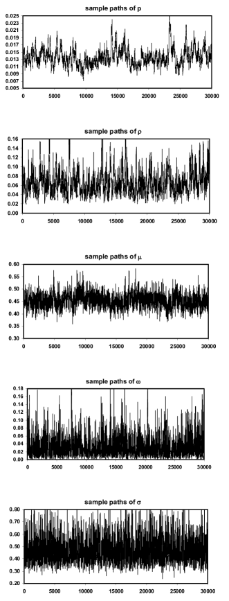
Figure 2: Markov chain Monte Carlo sample paths for parameters $(p,\rho,\mu,\omega,\sigma)$ for the case of the 1982-1999 dataset.

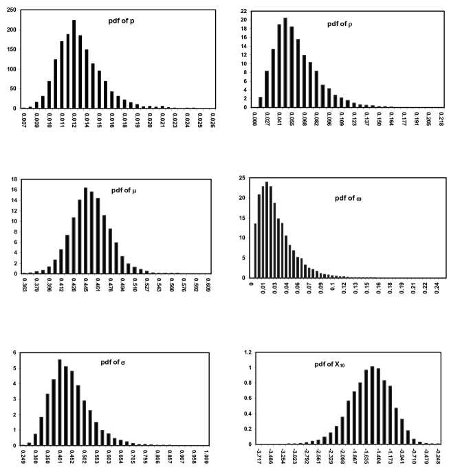
Figure 3: Posterior density functions for the model parameters $(p,\rho,\mu,\sigma,\omega)$ and systematic factor $X_{10}$ (corresponding to the year of 1991), computed from MCMC samples for the 1982-1999 dataset.

The posterior sample paths (after the burn-in) for parameters $(p,\rho,\mu,\omega,\sigma)$ are shown in Figure 2. All paths reveal well-mixed MCMC samples indicative of stationary distributions, as expected for a convergent MCMC simulation. Figure 3 shows the posterior density functions estimated from the posterior samples for parameters $(p,\rho,\mu,\omega,\sigma)$ and one of the 18 latent variables $X_{10}$. Clearly, the densities show some positive skewness for all parameters and negative skewness for $X_{10}$. Table 3 shows the summary statistics of all five parameters computed from the posterior samples – the mode, mean, standard deviation (stdev), skewness and kurtosis. To quantify uncertainty in a simple manner, the coefficient of variation (CV), defined as the ratio of standard deviation to the mean, is also shown in Table 3. Consistent with Figure 3, we see significant positive skewness in most parameters; kurtosis values of some parameters are significantly larger than three (kurtosis of a normal density). This also indicates that Gaussian approximation for parameter uncertainties (typically used under the frequentist maximum likelihood method) is not appropriate.

5.3 Impact of Parameter Uncertainty on Quantile Estimate

Comparison between Tables 2 and 3 shows that the closed-form MLEs for all parameters are within one standard deviation from the posterior mean.

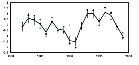
Figure 4: Posterior mean (given data) for the systematic factor $X_{t},t=1,\ldots,18$ (solid line) in comparison with the maximum likelihood point estimates (dots), corresponding to the 1982-1999 dataset. Error bars correspond to posterior standard deviation of $X_{t}$.

The comparison for the 18 latent variables of systematic factor (for 18 years of data between 1982-1999) $X_{t},t=1,\ldots,18$ is shown in Figure 4. Here, $X_{t}$ implied by MLEs (22) agrees well with the corresponding posterior sample mean – only one point is more than one standard deviation away from the posterior mean.

A very large difference in model parameters does not always imply a large difference in model predictions. The predictions on the stressed PD, LGD and EC are shown in Table 2 for MLE and Table 4 for MCMC. The quantiles in Table 4 were obtained from Algorithm 3. For a comparison between point estimates, the point estimates for PD, LGD and EC using the posterior mean $\hat{\bm{\theta}}^{\tiny{\mbox{MMSE}}}=E[{\bm{\theta}}|{\bm{Y}}]$ (instead of MLEs) are

$$PD(\hat{\bm{\theta}}^{\tiny{\mbox{MMSE}}})=0.0682,\quad LGD(\hat{\bm{\theta}}^{\tiny{\mbox{MMSE}}})=0.776\quad\mbox{and}\quad Q^{\infty}_{0.999}(\hat{\bm{\theta}}^{\tiny{\mbox{MMSE}}})=0.054.$$

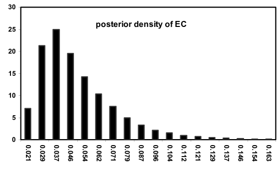
Figure 5: Posterior density of economic capital $EC^{\infty}=Q^{\infty}_{0.999}({\bm{\Theta}})$ computed from MCMC samples using Algorithm 3 for the 1982-1999 dataset.

The posterior density of EC is shown in Figure 5. Evidently the distribution is positively skewed. Comparison of Table 2 and 4 shows that for the EC as defined in (11), the MLE point estimate (in closed form) is $58\%$ lower than the posterior mean from MCMC, $41\%$ lower than the posterior median and about $90\%$ lower than the 0.75 quantile. The MLE is within one standard deviation from the posterior mean. However, note that the uncertainty (due to small data size) is very large, CV is about 42%; also note a large difference between the 0.75 and the 0.25 quantiles of EC posterior. Given that posterior density of EC is skewed, CV is not a good measure of parameter uncertainty and it is better to use posterior quantiles for this purpose. The underestimation of EC by the MLE in comparison with Bayesian posterior estimates is quite significant, and this is the consequence of large parameter uncertainty, and large skeweness in posterior of EC. The latter also indicates that the use of the error propagation method based on the first-order Taylor expansion to estimate the error in EC via the errors in parameters (typically used under the frequentist approach) would not be appropriate.

5.4 Quantile Estimate via Full Predictive Loss Distribution

Table 5 shows the 0.999 quantile ${Q}^{P}_{0.999}$ of the full predictive loss density $f_{L_{T+1}}(\cdot|\bm{y})$ (the density of loss given data only, where parameters are integrated out; see Section 4.1), in the case of portfolios with a different number of borrowers $J$ assuming equal weights $w_{1}=\cdots=w_{J}=1/J$. The highest number $J=5000$ is close to the actual number of firms in the last year of the 18 year dataset. The qauntiles ${Q}^{P}_{0.999}$ in Table 5 were computed using Algorithm 2. At $J=\infty$, instead of using Step 2 of Algorithm 2, the loss $L$ is calculated using formula (10) for the limiting case of a large portfolio. Clearly from Table 5, the quantile $Q^{P}_{0.999}$ decreases with the number of firms $J$, reaching a limiting value at $J=\infty$. The smaller quantile for the loss distribution of a larger portfolio is a diversification effect. For instance for the period 1982-1999, at $J=500$ the full predictive quantile $Q^{P}_{0.999}$ is about $30\%$ lower than the case at $J=50$; the quantile $Q^{P}_{0.999}$ for the limiting case $J=\infty$ is about $4\%$ lower than for the $J=500$ case.

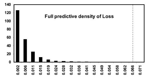
Figure 6: The full predictive density (accounting for parameter uncertainty) of the total loss $L^{\infty}_{T+1}$ computed from MCMC samples using Algorithm 2 for the 1982-1999 dataset. Dashed line indicates the 0.999 quantile, $Q^{P}_{0.999}$.

The posterior density of the full predictive distribution for $L^{\infty}$ is shown in Figure 6. The quantile of full predictive distribution ${Q}^{P}_{0.999}$ at $J=\infty$ is more than twice as large as the $EC^{\infty}$ estimated by the approximate MLE (shown in Table 2), and it is also $30\%$ larger than the posterior mean of $Q^{\infty}_{0.999}({\bm{\Theta}})$ (shown in Table 4). This illustrates that parameter uncertainty is very significant in determining economic capital in the one-factor credit risk model studied here, which is not surprising given a small dataset of annual defaults and recoveries over 18 years. Also, this shows that the use of MLE may lead to a very significant underestimation in EC.

To account for parameter uncertainty (due to finite sample size), we suggest that EC should be measured as the quantile ${Q}^{P}_{q}$ of the full predictive loss distribution rather than some point estimates based on MLEs or characteristics of the posterior for $Q^{\infty}_{q}({\bm{\Theta}})$. The extra loading in EC due to parameter uncertainty can be defined by (44), i.e. the difference between ${Q}^{P}_{0.999}$ and posterior mean of $Q^{\infty}_{0.999}({\bm{\Theta}})$.

6 Results for 1982-2010 Dataset

In this section we show MCMC and MLE results based on the default and recovery data (presented in Table 1) covering the 1982-2010 period, in which the worst financial crisis since the Great Depression of the 1930 occurred. The historical data for corporate default and recovery rates were taken from Moody’s (2011). The year 1982 is the earliest year for the recovery data provided in the Moody’s report. Also note that Moody’s and Standard&Poor’s data for 1982-1999 period are almost the same.

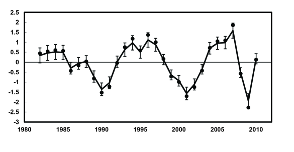
Figure 7: Posterior mean (given data) of systematic factor $X_{t},t=1,\ldots,29$ (solid line) in comparison with the maximum likelihood point estimates (dots), corresponding to the 1982-2010 dataset. Error bars correspond to posterior standard deviation of $X_{t}$.

The longer time period 1982-2010 has 11 extra recent years compared with the earlier period 1982-1999 considered in Section 5. Using this longer dataset, the closed-form MLE results for default and recovery parameters and the corresponding values for the the stressed probability of default PD, the stressed LGD and the economic capital EC are shown in Table 2. The results for 1982-2010 dataset certainly have higher probability of default PD, higher loss in terms of LGD and higher economic capital EC when compared to the results obtained from 1982-1999 dataset. Obviously, this is due to the global financial crisis occurred in recent years. The systematic factor $X_{t}$ for 2009 was found to be -2.27, which corresponds to approximately $99\%$ quantile level of the limiting loss distribution of the diversified portfolio. This maximum negative systematic factor for 2009 is the consequence of the disastrous 2008 when the bankruptcy of Lehman Brothers occurred (the largest bankruptcy filing in U.S. history). The comparison for the 29 latent variables $X_{t},t=1,\ldots,29$ (corresponding to 29 years of 1982-2010 dataset) is shown in Figure 7. The systematic factor $X_{t}$ implied by MLE parameter values (22) again agrees well with the posterior sample mean of MCMC; all maximum likelihood point estimates are within one standard deviation from the posterior mean.

The summary statistics (mode, mean, standard deviation, skewness, kurtosis and the coefficient of variation) of all five model parameters computed from the posterior samples for the 1982-2010 dataset are shown in Table 3. Similar to the period of 1982-1999, we see significant positive skewness in most parameters. In addition, the kurtosis values of some parameters are significantly higher than kurtosis of a normal density.

Results for the 1982-2010 dataset also show that the closed-form MLEs for all parameters are within one standard deviation from the posterior mean (see Tables 2 and 3). Again the closed-form MLE solution for $\sigma$ is close to the posterior mean for the 1982-2010 dataset. The MCMC predictions on stressed PD, LGD and EC for the 1982-2010 dataset are also shown in Table 4. Comparison shows that the closed-form MLE for EC is $35\%$ lower than the posterior mean, $24\%$ lower than the posterior median and more than $50\%$ lower than the 0.75 quantile of the posterior for EC. Similar to the period 1982-1999, the uncertainty in the posterior of EC is large, CV is about 34.5%, even though the sample data size has increased from 18 years to 29 years. Nevertheless, the increased data size has resulted in a reduction in uncertainty, as is evident in the reduction of CV. The ratio of CV (standard deviation normalized by the mean) of EC for the two time periods is $0.423/0.345\approx 1.23$ (see Table 4), while the square-root ratio of the data sizes for the corresponding time periods is $\sqrt{29/18}\approx 1.27$. This reduction in uncertainty approximately proportional to the square root of the data size is typically observed in statistical models, though generally speaking is valid in the limit of large data size.

The 0.999 quantile ${Q}^{P}_{0.999}$ of the full predictive loss density $f_{L_{T+1}}(\cdot|\bm{y})$ for the time period 1982-2010 for several portfolios with different number of borrowers $J$ is shown in Table 5. Similar to the time period 1982-1999, the diversification effect when increasing the number of firms from a small base is evident. The quantile ${Q}^{P}_{0.999}$ decreases with $J$ reaching a limiting value at $J=\infty$. As shown in Table 5 for the period 1982-2010, $Q^{P}_{0.999}$ at $J=500$ is about $25\%$ lower than the case at $J=50$; and for $J=5000$ is virtually the same as for the limiting case $J=\infty$. Also, note that ${Q}^{P}_{0.999}$ at $J=\infty$ is about 50% larger than corresponding MLE in Table 2; and about 15% larger than the posterior mean of $Q^{\infty}_{0.999}({\bm{\Theta}})$ in Table 4 (also see formula (44)), which is a significant reduction when compared to the results for $1982-1999$ dataset. The 15% impact of parameter uncertainty on the 0.999 quantile of the loss distribution gives indication that $1982-2010$ dataset is long enough for the use of the calibrated LGD model. In comparison, it would be difficult to justify the use of the model with the $1982-1999$ dataset where the impact of parameter uncertainty is too large.

7 Conclusion

This paper presents a methodology of estimating the default and recovery model parameters and latent systematic risk factors in the well known LGD model via Bayesian approach and Markov chain Monte Carlo method. Under this approach, the uncertainty in parameters and model predictions is quantified using the posterior distribution obtained from the prior and data likelihood. Moreover, it allows an easy calculation of the full predictive loss density $f_{L_{T+1}}(\cdot|\bm{y})$ accounting for parameter uncertainty as described in Section 4.1; then the economic capital can be based on the high quantile of this distribution $Q_{q}^{P}$.

Given small datasets typically used to fit the model, the parameter uncertainty is large and the posterior is very different from the normal distribution indicating that Gaussian approximation for parameter uncertainties (typically used under the frequentist maximum likelihood approach assuming large sample limit) is not appropriate. As an illustration, using Moody’s and Standard&Poor’s data for the annual corporate default and recovery rates, we calibrated the model and quantified the impact of parameter uncertainty on economic capital as if this dataset would correspond to the dataset of the real bank portfolio. The posterior mean of economic capital $Q_{0.999}^{\infty}(\bm{\Theta})$ is 35% higher than corresponding MLE estimate for the longest 1982-2010 dataset, and 58% higher for the 1982-1999 dataset. In addition, the 0.999 quantile of the full predictive distribution $Q_{0.999}^{P}$ is more than twice as large as the MLE estimate of EC for 1982-1999 dataset and about 50% larger for 1982-2010 dataset. This strongly indicates that it is dangerous to use the MLE estimate for EC. The impact of parameter uncertainty on the quantile, see formula (44), quantified as the relative difference between $Q_{0.999}^{P}$ and posterior mean of $Q_{0.999}^{\infty}(\bm{\Theta})$, is about 30% for 1982-1999 dataset and 15% for 1982-2010 dataset. These results demonstrate that the extra capital to cover parameter uncertainty can be significant and should not be disregarded by practitioners developing LGD models.

At this stage, datasets of default and recovery time series for bank loans are not available and thus the considered LGD model cannot be used for direct calculations of capital against real credit risk portfolios in banks. At the moment, PDs and LGDs are estimated from balance sheet information. Therefore our numerical results for EC and impact of parameter uncertainty on EC should be considered as an illustration of the method only.

The main objective of the paper is to demonstrate how the Bayesian approach and MCMC method can be used to estimate LGD model and related quantities. For simplicity we considered the case of homogeneous portfolio. It is not difficult to extend the approach and algorithm to deal with non-homogeneous portfolios and more than one latent factor. Macroeconomic factors such as GDP can be incorporated into the model similar to Rösch and Scheule (2005); also it should be worth to consider mean reversion in the systematic factor.

8 Acknowledgement

We would like to thank the anonymous referee for critical and constructive comments, Peter Thomson for useful discussions, and the credit risk quantitative team of Commonwealth Bank of Australia for influencing our knowledge of this subject.

Table 1: Global corporate default and recovery annual rates from Moody’s (2011). Data in brackets for 1982-1999 are Standard&Poor’s data used in Düllmann and Trapp (2004).

year	recovery rate	default rate	no. defaults	no. firms
1982	0.353 (0.358)	0.01036 (0.0119)	13 (18)	1255 (1513)
1983	0.445 (0.4925)	0.00967 (0.0068)	13 (11)	1344 (1618)
1984	0.455 (0.5331)	0.00927 (0.0083)	13 (13)	1402 (1566)
1985	0.436 (0.447)	0.00950 (0.0103)	15 (18)	1579 (1748)
1986	0.474 (0.3665)	0.01855 (0.0169)	33 (32)	1779 (1893)
1987	0.513 (0.5399)	0.01558 (0.0093)	31 (19)	1990 (2043)
1988	0.388 (0.4455)	0.01365 (0.0144)	29 (31)	2125 (2153)
1989	0.323 (0.4367)	0.02361 (0.0153)	52 (39)	2202 (2549)
1990	0.255 (0.2682)	0.03588 (0.0256)	82 (66)	2285 (2578)
1991	0.355 (0.4702)	0.03009 (0.0306)	66 (89)	2193 (2908)
1992	0.459 (0.5388)	0.01434 (0.0122)	31 (33)	2162 (2705)
1993	0.431 (0.502)	0.00836 (0.0051)	19 (23)	2273 (4510)
1994	0.456 (0.5609)	0.00614 (0.0052)	16 (18)	2606 (3462)
1995	0.433 (0.4988)	0.00935 (0.0091)	27 (33)	2888 (3626)
1996	0.415 (0.4534)	0.00533 (0.0045)	17 (20)	3189 (4444)
1997	0.488 (0.564)	0.00698 (0.006)	25 (24)	3582 (4000)
1998	0.383 (0.415)	0.01255 (0.0118)	51 (56)	4064 (4746)
1999	0.338 (0.3207)	0.02214 (0.02)	100 (107)	4517 (5350)
2000	0.253	0.02622	124	4729
2001	0.216	0.03978	187	4701
2002	0.297	0.03059	141	4609
2003	0.404	0.01844	82	4447
2004	0.585	0.00855	38	4444
2005	0.560	0.00674	31	4599
2006	0.550	0.00654	31	4740
2007	0.547	0.00367	18	4905
2008	0.339	0.02028	103	5079
2009	0.339	0.05422	265	4887
2010	0.500	0.01283	57	4443

Table 2: Maximum likelihood estimates of the model parameters and corresponding estimates of stressed PD, LGD and EC using approximate likelihood function (24) for default and (29) for recovery data. Here, EC is estimated as $Q^{\infty}_{0.999}(\hat{\bm{\theta}}^{MLE})$ in (11) with $\hat{\bm{\theta}}^{MLE}$ is the maximum likelihood point estimate for $\bm{\theta}$.

Time period	$p$	$\rho$	$\mu$	$\sigma$	$\omega$	PD	LGD	EC
1982-1999	0.0123	0.0406	0.450	0.445	0.0118	0.0488	0.710	0.0346
1982-2010	0.0167	0.0635	0.411	0.499	0.0192	0.0819	0.813	0.0666

Table 3: Summary statistics of the model parameters $(p,\rho,\mu,\omega,\sigma)$ from posterior MCMC samples. Stdev is the standard deviation, and CV is the coefficient of variation.

Time period	item	Mode	Mean	Stdev	Skewness	Kurtosis	CV
	$p$	0.0157	0.0133	0.0022	0.951	4.86	0.168
	$\rho$	0.143	0.0623	0.0239	1.07	4.74	0.376
1982-1999	$\mu$	0.471	0.456	0.027	0.221	3.64	0.058
	$\omega$	0.060	0.032	0.023	1.72	8.32	0.711
	$\sigma$	0.448	0.457	0.085	0.912	4.50	0.183
	$p$	0.0177	0.0179	0.0028	0.812	4.62	0.154
	$\rho$	0.141	0.0815	0.024	1.01	4.35	0.286
1982-2010	$\mu$	0.439	0.414	0.022	0.309	3.19	0.055
	$\omega$	0.0717	0.031	0.016	1.24	5.39	0.51
	$\sigma$	0.449	0.502	0.070	0.588	3.63	0.140

Table 4: Summary statistics from posterior MCMC samples for the stressed PD, LGD and EC, i.e. calculated assuming systematic factor $x_{T+1}=\Phi^{-1}(0.001)$. $\delta$EC($\%$) is the relative difference between each quantile value of the distribution of $Q^{\infty}_{\alpha}({{\bm{\Theta}}})$ calculated using Algorithm 3 and EC value estimated by MLE, $Q^{\infty}_{0.999}({\hat{\bm{\theta}}^{MLE}})$, where $\hat{\bm{\theta}}^{MLE}$ is the maximum likelihood estimate for $\bm{\theta}$.

Time period	item	Mean	Stdev	0.25Q	0.5Q	0.75Q	CV
	PD	0.0682	0.0236	0.0513	0.0629	0.0800	0.346
1982-1999	LGD	0.786	0.0745	0.733	0.777	0.829	0.0947
	$Q^{\infty}_{0.999}({\bm{\Theta}})$	0.0547	0.023	0.0385	0.0489	0.0652	0.420
	$\delta$EC($\%$)	58.1$\%$	N/A	11.3$\%$	41.3$\%$	88.4$\%$	N/A
	PD	0.103	0.029	0.0825	0.0968	0.116	0.288
1982-2010	LGD	0.858	0.0542	0.820	0.852	0.889	0.064
	$Q^{\infty}_{0.999}({\bm{\Theta}})$	0.0891	0.031	0.0683	0.0824	0.102	0.348
	$\delta$EC($\%$)	33.8$\%$	N/A	2.55$\%$	23.7$\%$	53.8$\%$	N/A

Table 5: Full predictive quantile $Q^{P}_{0.999}$ for various portfolios (different number of borrowers) using Algorithm 2.

Time period	$J=50$	$J=500$	$J=5000$	$J=\infty$
1982-1999	0.1044	0.0742	0.0732	0.0709
1982-2010	0.1454	0.1092	0.1026	0.1026

References

- [1] Altman, E. I. Default recovery rates and LGD in credit risk modeling and practice: an updated review of the literature and empirical evidence. Preprint (November 2006). http://people.stern.nyu.edu/ealtman/UpdatedReviewofLiterature.pdf.
- [2] Basel Committee on Banking Supervision. Guidance on Paragraph 468 of the Framework Document. Bank for International Settlements, Basel, July 2005.
- [3] Berger, J. O. Statistical Decision Theory and Bayesian Analysis. Springer-Verlag, New York, 1985.
- [4] Bluhm, C., Overbeck, L., and Wagner, C. An Introduction to Credit Risk Modeling. Chapman & Hall/CRC, 2002.
- [5] Bolstad, W. M. Introduction to Bayesian Statistics. John Wiley, 2004.
- [6] Cantor, R., and Varma, P. Determinants of recovery rates on defaulted bonds and loans for north american corporate issuers: 1983-2003. The Journal of Fixed Income 14, 4 (2005), 29–44.
- [7] Carlin, B. P., and Louis, T. A. Bayesian Methods for Data Analysis. Chapman & Hall/CRC, 2008.
- [8] Credit Suisse Financial Products. Creditrisk+: a credit risk management framework. Technical document (1997).
- [9] Denuit, M., Dhaene, J., Goovaerts, M. J., and Kaas, R. Actuarial Theory for Dependent Risks. Wiley, Chichester, 2005.
- [10] Düllmann, K., and Trapp, M. Systematic risk in recovery rates - an empirical analysis of us corporate credit exposures. Discussion Paper, Series2: Banking and Financial Supervision (2004), 1–44.
- [11] Frye, J. Collateral damage. Risk 4 (2000a), 91–94.
- [12] Frye, J. Depressing recoveries. Risk 13 (2000b), 106–111.
- [13] Gelman, A., Carlin, J., Stern, H., and Rubin, D. B. Bayesian Data Analysis. Chapman & Hall/CRC, Boca Raton, Florida, 2003.
- [14] Gelman, A., Gilks, W. R., and Roberts, G. O. Weak convergence and optimal scaling of random walk Metropolis algorithm. Annals of Applied Probability 7 (1997), 110–120.
- [15] Gordy, M. A risk-factor foundation for ratings-based bank capital rules. Finance and Economics Discussion Series 2002-55, Washington: Board of Governors of the Federal Reserve System (2002).
- [16] Gupton, G., Finger, C., and Bhatia, M. Creditmetrics - technical document. Morgan Guaranty Trust Co. (1997). http://www.creditmetrics.com.
- [17] Luo, X., Shevchenko, P. V., and Donnelly, J. Addressing impact of truncation and parameter uncertainty on operational risk estimates. The Journal of Operational Risk 2, 4 (2007), 3–26.
- [18] Metropolis, N., Rosenbluth, A. W., Rosenbluth, M. N., Teller, A. H., and Teller, E. Equations of state calculations by fast computing machines. Journal of Chemical physics 21 (1953), 1087–1091.
- [19] Moody’s. Corporate default and recovery rates, 1920-2010. Technical report, February 2011.
- [20] Peters, G. W., Shevchenko, P. V., and Wüthrich, M. V. Model uncertainty in claims reserving within Tweedie’s compound poisson models. ASTIN Bulletin 39, 1 (2009a), 1–33.
- [21] Peters, G. W., Shevchenko, P. V., and Wüthrich, M. V. Dynamic operational risk: modelling dependence and combining different data sources of information. The Journal of Operational Risk 4, 2 (2009b), 69–104.
- [22] Pykhtin, M. Unexpected recovery risk. Risk 16, 8 (2003), 74–78.
- [23] Robert, C. P. The Bayesian Choice. Springer Verlag, New York, 2001.
- [24] Roberts, G. O., and Rosenthal, J. S. Optimal scaling for various Metropolis-Hastings algorithms. Statistical Science 16 (2001), 351–367.
- [25] Roberts, G. O., and Smith, A. F. Simple conditions for the convergence of the Gibbs sampler and Metropolis Hastings algorithms. Stochastic Processes and their Applications 49 (1994), 207–216.
- [26] Rösch, D., and Scheule, H. A multifactor approach for systematic default and recovery risk. The Journal of Fixed Income 15, 2 (2005), 63–75.
- [27] Schönbucher, P. J. Factor models for portfolio credit risk. Journal of Risk Finance 3, 1 (2001), 45–56.
- [28] Shevchenko, P. V. Estimation of operational risk capital charge under parameter uncertainty. The Journal of Operational Risk 3, 1 (2008), 51–63.
- [29] Shevchenko, P. V. Modelling Operational Risk Using Bayesian Inference. Springer, Berlin, 2011.
- [30] Shevchenko, P. V., and Temnov, G. Modeling operational risk data reported above a time-varying threshold. The Journal of Operational Risk 4, 2 (2009), 19–42.
- [31] Standard&Poor’s. Corporate defaults peak in 2002 amid record amounts of defaults and declining credit quality. Standard&Poor’s Special Report 5-49, February 2003.
- [32] Winkler, R. L. Introduction to Bayesian Inference and Decision. Probabilistic, 2003.