Hyperfine-mediated static polarizabilities of monovalent atoms and ions

Abstract

We apply relativistic many-body methods to compute static differential polarizabilities for transitions inside the ground-state hyperfine manifolds of monovalent atoms and ions. Knowing this transition polarizability is required in a number of high-precision experiments, such as microwave atomic clocks and searches for CP-violating permanent electric dipole moments. While the traditional polarizability arises in the second-order of interaction with the externally-applied electric field, the differential polarizability involves additional contribution from the hyperfine interaction of atomic electrons with nuclear moments. We derive formulas for the scalar and tensor polarizabilities including contributions from magnetic dipole and electric quadrupole hyperfine interactions. Numerical results are presented for Al, Rb, Cs, Yb⁺, Hg⁺, and Fr.

I Introduction

When an atom is placed in an external electric field, its energy levels shift due to the Stark effect. For states of definite parity, the effect arises in the second order in the interaction of atomic electrons with the external E-field. The energy shift $\delta E_{a}$ is conventionally parameterized in terms of the polarizability of the atomic state $\alpha_{a}$,

$$\delta E_{a}=-\frac{1}{2}\alpha_{a}\mathcal{E}_{0}^{2}\,,$$ (1)

where $\mathcal{E}_{0}$ is the strength of the applied E-field.

The polarizability depends on atomic electric-dipole $D$ matrix elements and energies $E$

$$\alpha_{a}=2\,\sum_{b\neq a}\frac{\left|\langle a|D_{z}|b\rangle\right|^{2}}{E_{b}-E_{a}}\,.$$ (2)

The sums are over a complete atomic eigen-set and the $z$-axis has been chosen along the E-field. On general grounds, we may decompose the polarizability for a state $|nFM_{F}\rangle$ of the total angular momentum $F$ and its projection $M_{F}$ into the following contributions,

$$\alpha_{nFM_{F}}=\alpha_{nF}^{S}+\frac{3{M_{F}}^{2}-F(F+1)}{F(2F-1)}\alpha_{nF}^{T}\,.$$ (3)

Here the superscripts $S$ and $T$ distinguish the scalar and tensor parts of the polarizability. The “polarizabilities” $\alpha_{nF}^{S}$ and $\alpha_{nF}^{T}$ no longer depend on the magnetic quantum number $M_{F}$.

In this paper we focus on a difference of polarizabilities between two states $nF^{\prime}$ and $nF$ of the same hyperfine manifold of states of total orbital angular momentum $J=1/2$. Such calculations require additional care. Indeed, we are considering the Stark shift of hyperfine levels attached to the same electronic state. To the leading order, the shift is determined by the properties of the underlying electronic state. However, because the electronic state for both hyperfine levels is the same, the scalar Stark shift of both levels is the same. An apparent difference between the two levels is caused by the hyperfine interaction (HFI), and the rigorous analysis involves so-called HFI-mediated polarizabilities (see, e.g., RosGheDzu09 ). Similar arguments hold for the tensor part of the polarizability. $\alpha_{nF}^{T}$, taken with its prefactor in Eq. (3 ), is an expectation value of an irreducible tensor operator of rank 2; it simply vanishes for $J=1/2$ states due to the angular selection rules. Only the HFI coupling of nuclear and electronic momenta ($\mathbf{F}=\mathbf{I}+\mathbf{J}$) leads to nonzero values of the tensor polarizability.

Early works on Stark shifts of transition frequencies within hyperfine manifolds include Refs. HauZac57 ; LipSan64 ; San67 ; CarAdlBak68 ; GouLipWei69 . More recent interest to this problem was motivated by the Stark shifts of the hyperfine transition frequency due to the ambient black-body radiation (BBR) ItaLewWin82 . The BBR shift is a major systematic correction in microwave clocks, especially the ¹³³Cs primary frequency standard WynWey05 . This motivated the most precise measurement of the DC Stark shift in a Cs fountain SimLauCla98 . The relevant Stark shifts were a subject of many recent works (see, e.g., state-of-the-art calculations Ref. BelSafDer06 ; AngDzuFla06PRL and references therein).

Perhaps the most complete earlier theoretical treatment within the third-order (two electric-dipole couplings and one HFI) perturbation theory was given by Sandars San67 in 1967. However, only recently (i.e., four decades later), a sign mistake in the expression of Ref. San67 for the tensor part of the HFI-mediated polarizability was discovered UlzHofMor06 ; HofMorUlz08 (a correct result for tensor polarizability of Tl was obtained earlier in Ref. SkoFla78 ).

This sign error is directly relevant to extracting BBR correction from high-precision experiments. Notice that due to the isotropic nature of the BBR, the BBR clock shift is expressed in terms of the scalar part of the HFI-mediated polarizability. Moreover, characteristic frequencies of room-temperature BBR are well below excitation energies of atomic transitions thereby justifying replacing frequency-dependent polarizability with DC polarizability ItaLewWin82 . Accordingly, the modern value of the BBR correction for the Cs clock is based on a measurement SimLauCla98 which was carried out in a DC E-field. However, the measured Stark shift involves a combination (3) of both scalar and tensor polarizabilities. Therefore to arrive at the BBR shift, one needs to remove the contribution due to the tensor polarizability. Clearly, the sign mistake discovered in UlzHofMor06 ; HofMorUlz08 becomes relevant.

Here we extend our earlier treatment of the HFI-mediated polarizabilities BelSafDer06 ; AngDzuFla06PRL ; RosGheDzu09 with a specific focus on the tensor polarizabilities. Compared to Refs. UlzHofMor06 ; HofMorUlz08 we employ a fully-relativistic formalism and evaluate tensor polarizabilities for several atoms and ions using modern relativistic many-body methods. We independently confirm that indeed, Ref. San67 had a sign mistake, requiring reinterpretation of measurements SimLauCla98 . We also evaluate the tensor polarizability for the secondary frequency standard based on Rb atoms.

Another motivation for our work comes from searches for the so far elusive permanent electric-dipole moments (EDM). Non-vanishing EDMs violate both time- and parity-reversal symmetries. Planned experiments will be carried out with Fr atoms FrEDM . These atoms will be placed in a strong electric field and so-far unknown $M_{F}$-dependent tensor polarizabilities would contribute to the error budget of the EDM search. Our computed values for Fr isotopes will aid the design and interpretation of these planned experiments.

The paper is organized as follows. In Section II we derive fully-relativistic third-order formulae for HFI-mediated tensor polarizabilities. Section III presents details of numerical evaluation within relativistic many-body theory. Finally, the results are discussed and compared with literature values in Section IV. Unless specified otherwise, atomic units, $m_{e}=\hbar=|e|=1$ are used throughout.

II Theoretical setup

We are interested in transitions between two hyperfine components of the same electronic states. Below we employ the conventional labeling scheme for the atomic eigenstates, $\left|n\left(IJ\right)FM_{F}\right\rangle$, where $I$ is the nuclear spin, $J$ is the electronic angular momentum, and $F$ is the total angular momentum, $\mathbf{F}=\mathbf{J}+\mathbf{I}$. $M_{F}$ is the projection of $F$ on the quantization axis and $n$ encompasses the remaining quantum numbers.

As discussed in the introduction, computation of the transition polarizability for $J=1/2$ hyperfine-manifolds requires third-order analysis. This involves two perturbations due to the externally-applied electric field, $V_{E}=-\mathbf{D}\cdot\mathcal{E}$, and hyperfine interaction $V_{\mathrm{HFI}}$. These perturbations may be chained into three distinct diagrams (see Fig. 1). Additionally, there is a residual (or normalization) diagram.

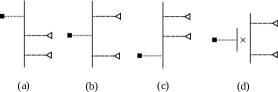
Figure 1: Diagrams representing the complete third order hyperfine-mediated polarizability. Each diagram contains a hyperfine interaction (dotted line capped with a filled square) in addition to two interactions with the external electric field (dashed line capped with an empty triangle). The diagrams correspond to the (a) top, (b) center, (c) bottom, and (d) normalization terms discussed in the text.

We would like to stress the importance of a consistent treatment of the HFI-mediated polarizabilities (i.e., including all the diagrams in Fig. 1). Consider a general expression for the scalar polarizability,

$$\alpha_{nF}^{S}=\frac{2}{3}\sum_{k=x,y,z}\sum_{i=|n_{i}F_{i}M_{i}\rangle}\frac{\langle nFM_{F}|~{}D_{k}|i\rangle\langle i~{}|D_{k}|nFM_{F}\rangle}{E_{nFM_{F}}-E_{i}}.$$ (4)

Here all the involved states are the hyperfine states. While this requires that the energies include hyperfine splittings, it also means that the wave-functions incorporate HFI to all orders of perturbation theory. Including the experimentally-known hyperfine splittings in the summations is straightforward but limiting ourselves to this approximation would exclude the HFI corrections to the wave-functions. By expanding the energy denominators, we observe that including HFI into energies would only recover the residual diagram and partially the center diagram. We find that the remaining contributions are of the same order, and limiting computations to HFI-induced energy shifts only is hardly justified.

Previously, we derived equations for dynamic HFI-mediated polarizabilities of hyperfine states in Ref. RosGheDzu09 . Clearly, static polarizabilities can be obtained by setting laser frequency to zero in the derived formulas. There is, however, one important addition to the formulae presented in Ref. RosGheDzu09 : the HFI operator in that paper was truncated at the magnetic-dipole interaction. Here we additionally include the HFI coupling due to the electric-quadrupole nuclear moment. This contribution to tensor polarizabilities becomes increasingly important for heavier atoms. Note that the electric quadrupole contribution to scalar polarizabilities and thermal shift of states with total momentum $j=1/2$ is zero. This can be explained in the following way. Scalar polarizability can be separated from total energy shift by averaging over directions of electric field. One cannot make non-zero scalar (energy shift is a scalar) from remaining electron angular momentum 1/2 and nuclear quadrupole, $j_{a}j_{b}Q_{ab}=\sigma_{a}\sigma_{b}Q_{ab}=0$ (squared Pauli matrix sigma is reduced to delta symbol and antisymmetric linear tensor with $\sigma$, $Q_{ab}$ is symmetric with zero trace, so that $\sum_{a}Q_{aa}=0$).

On general grounds, the rotationally-invariant hyperfine interaction between atomic electrons and nuclear moments may be written as a sum over scalar products of irreducible tensor operators (we follow notation of Ref. Joh07book )

$$V_{\mathrm{HFI}}=\sum_{N}\mathcal{N}^{\left(N\right)}\cdot\mathcal{T}^{\left(N\right)}\,.$$ (5)

Here the irreducible tensor operators $\mathcal{N}^{\left(N\right)}$ and $\mathcal{T}^{\left(N\right)}$ act in the space of nuclear and electronic coordinates respectively, with $N$ being their ranks. The nuclear magnetic moment is conventionally defined as

$$\mu=\langle I,M_{I}=I|\mathcal{N}_{0}^{\left(1\right)}|I,M_{I}=I\rangle$$ (6)

and the nuclear electric-quadrupole moment as

$$Q=2\langle I,M_{I}=I|\mathcal{N}_{0}^{\left(2\right)}|I,M_{I}=I\rangle\,.$$ (7)

In the formulas below we require the reduced matrix element of the nuclear moment operator in the nuclear basis. For magnetic dipole, this is related to the nuclear magnetic $g$-factor as

$$\langle I||\mathcal{N}^{\left(1\right)}||I\rangle=\frac{1}{2}\sqrt{\left(2I\right)\left(2I+1\right)\left(2I+2\right)}~{}g\mu_{n},$$

$\mu_{n}$ being the nuclear magneton and $\mu=gI\mu_{n}$. For the electric-quadrupole moment,

$$\langle I||\mathcal{N}^{\left(2\right)}||I\rangle=\frac{\sqrt{\left(2I-2\right)!\left(2I+3\right)!}}{2\left(2I\right)!}\,Q\,.$$

The components of relevant electronic tensors are

$$\mathcal{T}_{\lambda}^{\left(1\right)} =-\frac{i\sqrt{2}\left(\mathbf{\alpha}\cdot\mathbf{C}_{1\lambda}^{\left(0\right)}\left(\mathbf{\hat{r}}\right)\right)}{cr^{2}}\,,$$

$$\mathcal{T}_{\lambda}^{\left(2\right)} =-\frac{C_{\lambda}^{2}\left(\mathbf{\hat{r}}\right)}{r^{3}}\,,$$

where $r$ is the electronic coordinate, $\mathbf{\alpha}$ are the Dirac matrices, and $\mathbf{C}_{1\lambda}^{\left(0\right)}\left(\mathbf{\hat{r}}\right)$ and $C_{\lambda}^{2}\left(\mathbf{\hat{r}}\right)$ are normalized vector spherical harmonic and normalized spherical harmonic functions, respectively VarMosKhe88 .

A derivation similar to Ref. RosGheDzu09 results in the scalar and the tensor polarizabilities given by (here $[F]=2F+1$)

$$\alpha_{nF}^{s} =\frac{1}{\sqrt{3}}\frac{1}{\sqrt{[F]}}\alpha_{nF}^{\left(0\right)},$$

$$\alpha_{nF}^{T} =-\left[\frac{2}{3}\frac{~{}\left(2F\right)\left(2F-1\right)}{\left(2F+1\right)\left(2F+2\right)\left(2F+3\right)}\right]^{1/2}\alpha_{nF}^{\left(2\right)}\,,$$

with the reduced polarizabilities $\alpha_{nF}^{\left(K\right)}$ being sums over values of individual diagrams of Fig. 1,

$$\alpha_{nF}^{\left(K\right)}=\sum_{N}(2\alpha_{nF;N}^{\left(K\right)}\left(\mathrm{T}\right)+\alpha_{nF;N}^{\left(K\right)}\left(\mathrm{C}\right)+\alpha_{nF;N}^{\left(K\right)}\left(\mathrm{O}\right))\,,$$ (8)

where we used the equality of the top and bottom diagrams.

The angular reduction of individual diagrams leads to expressions

1JaK}{KJJaIFF}TJa​Jb(K)(nJ,N),\displaystyle\sum_{J_{a}J_{b}}\left(-1\right)^{J+J_{a}}\left\{\begin{tabular}[c]{lll}$I$&$I$&$N$\\ $J_{a}$&$J$&$F$\end{tabular}\ \ \ \right\}\left\{\begin{tabular}[c]{lll}$J$&$1$&$J_{b}$\\ $1$&$J_{a}$&$K$\end{tabular}\ \ \ \right\}\left\{\begin{tabular}[c]{lll}$K$&$J$&$J_{a}$\\ $I$&$F$&$F$\end{tabular}\ \ \ \ \right\}T_{J_{a}J_{b}}^{\left(K\right)}\left(nJ,N\right),

$$\alpha_{nF;N}^{\left(K\right)}\left(\mathrm{T}\right) =[F]\sqrt{[K]}$$

J1Jb

$$\alpha_{nF;N}^{\left(K\right)}\left(\mathrm{C}\right)=[F]\sqrt{[K]} \sum_{J_{a}J_{b}}\sum_{J_{i}}[J_{i}](-1)^{2J_{a}+J_{b}+J+N-1}\times$$

$$\left\{\begin{array}[c]{ccc}J&J&J_{i}\\ I&I&N\\ F&F&K\end{array}\right\}\left\{\begin{array}[c]{ccc}J&J&J_{i}\\ J_{a}&J_{b}&N\\ 1&1&K\end{array}\right\}C_{J_{a}J_{b}}^{\left(K\right)}\left(nJ,N\right),$$

$$\alpha_{nF;N}^{\left(K\right)}\left(\mathrm{O}\right) =\left(-1\right)^{2J+1}\left\{\begin{array}[c]{ccc}N&I&I\\ F&J&J\end{array}\right\}\langle nJ||\mathcal{T}^{\left(N\right)}||nJ\rangle\langle I||\mathcal{N}^{\left(N\right)}||I\rangle\times$$

$$\left[F\right]\sqrt{\left[K\right]}\left\{\begin{array}[c]{ccc}J&J&K\\ F&F&I\end{array}\right\}\sum_{J_{a}}\left\{\begin{array}[c]{ccc}K&J&J\\ J_{a}&1&1\end{array}\right\}\times O_{J_{a}}^{\left(K\right)}\left(nJ\right).$$

Finally, the universal (these are independent on $F$, i.e., the clock level) reduced sums are

$$T_{J_{a}J_{b}}^{\left(K\right)}\left(nJ,N\right)=2\langle I||\mathcal{N}^{\left(N\right)}||I\rangle\sum_{n_{a},n_{b}\neq n}\frac{\langle nJ||\mathcal{T}^{\left(N\right)}||n_{a}J_{a}\rangle\langle n_{a}J_{a}||D||n_{b}J_{b}\rangle\langle n_{b}J_{b}||D||nJ\rangle}{\left(E-E_{a}\right)\left(E-E_{b}\right)}\,,$$ (9)

$$C_{J_{a}J_{b}}^{\left(K\right)}\left(nJ,N\right)=2\langle I||\mathcal{N}^{\left(N\right)}||I\rangle\sum_{n_{a},n_{b}\neq n}\frac{\langle nJ||D||n_{a}J_{a}\rangle\langle n_{a}J_{a}||\mathcal{T}^{\left(N\right)}||n_{b}J_{b}\rangle\langle n_{b}J_{b}||D||nJ\rangle}{\left(E-E_{a}\right)\left(E-E_{b}\right)}\,,$$ (10)

$$O_{J_{a}}^{\left(K\right)}\left(nJ\right)=2\sum_{n_{a}\neq n}\frac{\langle nJ||D||n_{a}J_{a}\rangle\langle n_{a}J_{a}||D||nJ\rangle}{\left(E-E_{a}\right)^{2}}\,.$$ (11)

In these sums the values of the total orbital momenta of intermediate states $J_{a}$ and $J_{b}$ are fixed.

III Numerical evaluation

To perform the calculations we use an ab initio approach which has been described in detail in Ref. AngDzuFla06 . In this approach high accuracy is attained by including important many-body and relativistic effects.

Calculations start from the relativistic Hartree-Fock (RHF) method in the $V^{N-1}$ approximation. This means that the initial RHF procedure is done for a closed-shell atomic core with the valence electron removed. After that, the states of the external electron are calculated in the field of the frozen core. Correlations are included by means of the correlation potential method DzuFlaSil87 . We use the all-order correlation potential $\hat{\Sigma}$ for Rb, Cs, and Fr and second-order correlation potential $\hat{\Sigma}^{(2)}$ for Al, Yb⁺, and Hg⁺. The all-order $\hat{\Sigma}$ includes two classes of the higher-order terms: screening of the Coulomb interaction and hole-particle interaction (see, e.g., DzuFlaSus89 for details).

To calculate $\hat{\Sigma}$ and $\hat{\Sigma}^{(2)}$ we need a complete set of single-electron orbitals. We use the B-spline technique JohBluSap88 to construct the basis. The orbitals are built as linear combinations of 40 B-splines of order 9 in a cavity of radius 40$a_{B}$. The coefficients are chosen from the condition that the orbitals are the eigenstates of the RHF Hamiltonian $\hat{H}_{0}$ of the closed-shell core. The all-order $\hat{\Sigma}$ operator is calculated with the technique which combines solving equations for the Green functions (for the direct diagram) with the summation over complete set of states (exchange diagram) DzuFlaSus89 . The second-order $\hat{\Sigma}^{(2)}$ operator is calculated using direct summation over complete set of states.

The correlation potential $\hat{\Sigma}$ is then used to build a new set of single-electron states, the so-called Brueckner orbitals. This set is to be used in the summation in equations (9), (10) and (11). Here again we use the B-spline technique to build the basis. The procedure is very similar to the construction of the RHF B-spline basis. The only difference is that new orbitals are now the eigenstates of the $\hat{H}_{0}+\hat{\Sigma}$ Hamiltonian.

Matrix elements of the HFI and electric dipole operators are found by means of the time-dependent Hartree-Fock (TDHF) method DzuFlaSil87 ; DzuFlaSus84 . This method is equivalent to the well-known random-phase approximation (RPA). In the TDHF method, the single-electron wave functions are presented in the form $\psi=\psi_{0}+\delta\psi$, where $\psi_{0}$ is the unperturbed wave function. It is an eigenstate of the RHF Hamiltonian $\hat{H}_{0}$: $(\hat{H}_{0}-\epsilon_{0})\psi_{0}=0$. $\delta\psi$ is the correction due to external field. It can be found be solving the TDHF equation

$$(\hat{H}_{0}-\epsilon_{0})\delta\psi=-\delta\epsilon\psi_{0}-\hat{F}\psi_{0}-\delta\hat{V}^{N-1}\psi_{0},$$ (12)

where $\delta\epsilon$ is the correction to the energy due to external field ($\delta\epsilon\equiv 0$ for the electric dipole operator), $\hat{F}$ is the operator of the external field ($V_{\mathrm{HFI}}$ or $-\mathbf{D}\cdot\mathcal{E}$), and $\delta\hat{V}^{N-1}$ is the correction to the self-consistent potential of the core due to external field.

The TDHF equations are solved self-consistently for all states in the core. Then the matrix elements between any (core or valence) states $n$ and $m$ are given by

$$\langle\psi_{n}|\hat{F}+\delta\hat{V}^{N-1}|\psi_{m}\rangle.$$ (13)

The best results are achieved when $\psi_{n}$ and $\psi_{m}$ are the Brueckner orbitals computed with the correlation potential $\hat{\Sigma}$.

We use equation (13) for all HFI and electric dipole matrix elements in evaluating the top, bottom, and center diagrams (Eqs. (9),(10),(11)) except for the ground state HFI matrix element in the normalization diagram where we use experimental data. The results are presented in section IV.

IV Results and Discussion

Table 1: Third-order hyperfine static polarizabilities of single-valence atoms.

$Z$	Atom	$A$	$I$	$\mu/\mu_{N}$	$Q$	$F$	$\alpha^{S}$	$\alpha_{A}^{T}$	$\alpha_{B}^{T}$	$\alpha^{T}$	$\alpha^{T}$
					[b]		$10^{-10}{\rm Hz}/({\rm V/m})^{2}$
13	Al	27	5/2	3.6415	0.14	3	0.0158	0.2683	-0.0119	0.2563
						2	-0.0222	-0.1073	-0.0096	-0.1169
37	Rb	85	5/2	1.3530	0.27	3	0.4599	-0.0073	-0.0070	-0.0143
						2	-0.6439	0.0029	-0.0056	-0.0027
37	Rb	87	3/2	2.7510	0.132	2	0.9332	-0.0148	-0.0034	-0.0182	-0.0234
						1	-1.5554	0.0025	-0.0017	0.0007	0.0009
55	Cs	133	7/2	2.5820	-0.004	4	1.9770	-0.0262	0.0002	-0.0260	-0.034
						3	-2.5419	0.0141	0.0002	0.0143	0.0184
70	Yb+	171	1/2	0.4940	1	1	0.0844	-0.0023	0	-0.0023
						0	-0.2533	0	0	0
70	Yb+	173	5/2	-0.6775	2.8	3	-0.1158	0.0031	-0.0390	-0.0359
						2	0.1621	-0.0012	-0.0312	-0.0325
80	Hg+	199	1/2	-0.5603	0.4	1	0.0271	-0.0018	0	-0.0018
						0	-0.0814	0	0	0
80	Hg+	201	3/2	0.5060	0.8	2	-0.0300	0.0020	-0.0014	0.0005
						1	0.0501	-0.0003	-0.0007	-0.0011
87	Fr	211	9/2	4.0005	-0.19	5	6.9771	-0.1459	0.0188	-0.1271	-0.1633
						4	-8.5275	0.0908	0.0175	0.1083	0.1392
87	Fr	221	5/2	1.5800	-0.98	3	2.7556	-0.0576	0.0970	0.0394	0.0506
						2	-3.8579	0.0230	0.0776	0.1006	0.129
87	Fr	223	3/2	1.1700	1.17	2	2.0406	-0.0427	-0.1158	-0.158	-0.204
						1	-3.4010	0.0071	-0.0579	-0.0508	-0.0653

Table 1 shows the results of calculation of scalar and tensor hyperfine mediated polarizabilities for two hyperfine components of the ground state of some isotopes of Al, Rb, Cs, Yb⁺, Hg⁺, and Fr. Magnetic dipole and electric quadrupole HFI contributions to the tensor polarizabilities ($\alpha^{T}$) are shown separately. Notice that there is no electric quadrupole contribution to the scalar polarizabilities ($\alpha^{S}$), as discussed previously. Another interesting thing to note is that electric quadrupole does not contribute to the frequency shift of the hyperfine transition. Although the tensor polarizabilities are different for states with $F=I+1/2$ and $F=I-1/2$, the energy shifts, which includes $F$-dependent factors (see Eq. (3)) are the same. This is only true for states with $M_{F}=0$, where $M_{F}$ is projection of $F$.

The accuracy of the calculations is different for scalar and tensor polarizabilities, being a few per cent for scalar polarizabilities and about 30% for tensor polarizabilities. This is because we include only Brueckner-type correlations, or correlations which can be reduced to redefinition of single-electron orbitals. Such approximation works very well for $s_{1/2}$ and $p_{1/2}$ states which dominate in the scalar polarizabilities. For tensor polarizabilities large contribution comes from $p_{3/2}$ and $d_{3/2}$ states where Brueckner approximation is not so good, especially for the HFI matrix elements. To get accurate results for tensor polarizabilities one has to include structure radiation and other non-Brueckner higher-order correlation corrections. This goes beyond the scope of present work.

To illustrate the accuracy of the calculations we would like to compare our results to previous calculations and available experimental data. There were numerous calculations and measurements of the Stark frequency shift for the hyperfine transitions of the ground state of Cs, Rb, and other atoms and ions (see, e.g., Ref. AngDzuFla06 and references therein). The results are usually presented in terms of the coefficient $k$ related to frequency shift by

$$\delta\Delta E=k\mathcal{E}_{0}^{2}\ ,$$ (14)

where $\Delta E$ is the energy interval between two hyperfine components of the ground state and $\delta\Delta E$ is its change due to electric field $\mathcal{E}_{0}$. One can find the values of $k$ for all atoms and ions from Table 1 using the polarizabilities from this table and expressions (1) and (3). Corresponding values for ⁸⁷Rb, ¹³³Cs, ¹⁷¹Yb⁺, and ¹⁹⁹Hg⁺ are presented in Table 2 and compared to previous calculations of Ref. AngDzuFla06 . Since both calculations are performed with the same method, we assume the same uncertainty. Some differences in central values for Yb and Hg are due to differences in the details of the calculations. These differences are within the declared uncertainty.

Table 2: Stark frequency shift: comparison with previous calculations.

Atom	$k,\ [10^{-10}{\rm Hz}/({\rm V/m})^{2}]$
	This work	Ref. AngDzuFla06
87Rb	-1.24(1)	-1.24(1)
133Cs	-2.26(2)	-2.26(2)
171Yb	-0.167(9)	-0.171(9)
199Hg	-0.056(3)	-0.060(3)

As has been discussed above the accuracy for the tensor polarizabilities is lower. Our value of the tensor polarizability for the $F=4$ state of cesium is $-2.60$ Hz(V/cm)². This is about 30% smaller that the experimental value $-3.34(2)(25)$ Hz(V/cm)² OspRasWeis03 and the semiempirical value $-3.72(25)$ Hz(V/cm)² HofMorUlz08 . The most likely reason for the difference is the contribution from the non-Brueckner correlations which are not included in present work. Therefore, we assume 30% uncertainty for the calculated tensor polarizabilities in present work.

To improve the predicted values for the tensor polarizabilities of Rb and Fr, which both have electron structure similar to those of cesium, we multiply the ab initio results for these atoms by the factor 1.28, which is the ratio of the experimental tensor polarizability for Cs to the theoretical one. The resulting values are presented in the last column of Table 1.

References

- (1) P. Rosenbusch, S. Ghezali, V. A. Dzuba, V. V. Flambaum, K. Beloy, and A. Derevianko, Phys. Rev. A 79, 013404 (2009)
- (2) R. D. Haun, Jr. and J. R. Zacharias, Phys. Rev. 107, 107–9 (1957)
- (3) E. Lipworth and P. G. H. Sandars, Phys. Rev. Lett. 13, 716 (1964)
- (4) P. G. H. Sandars, Phys. Rev. Lett. 19, 1396 (1967)
- (5) J. P. Carrico, A. Adler, M. R. Baker, S. Legowski, E. Lipworth, P. G. H. Sandars, T. S. Stein, and M. C. Weisskopf, Phys. Rev. 170, 64 (1968)
- (6) H. Gould, E. Lipworth, and M. C. Weisskopf, Phys. Rev. 188, 24 (1969)
- (7) Wayne M. Itano, L. L. Lewis, and D. J. Wineland, Phys. Rev. A 25, 1233-35 (1982)
- (8) R. Wynands and S. Weyers, Metrologia 42, S64 (2005)
- (9) E. Simon, P. Laurent, and A. Clairon, Phys. Rev. A 57, 436-39 (1998)
- (10) K. Beloy, U. I. Safronova, and A. Derevianko, Phys. Rev. Lett. 97, 040801 (2006)
- (11) E. J. Angstmann, V. A. Dzuba, and V. V. Flambaum, Phys. Rev. Lett. 97, 040802 (2006)
- (12) S. Ulzega, A. Hofer, P. Moroshkin, and A. Weis, Europhys. Lett. 76, 1074 (2006)
- (13) A. Hofer, P. Moroshkin, S. Ulzega, and A. Weis, Phys. Rev. A 77, 012502 (2008)
- (14) Y. I. Skovpen and F. V. V., Sov. Opt. Spectr. 45, 731 (1978)
- (15) http://www.fnal.gov/directorate/Longrange/Steering_Public/workshop-phys%ics-5th.html
- (16) W. R. Johnson, Atomic Structure Theory: Lectures on Atomic Physics (Springer, New York, NY, 2007)
- (17) D. A. Varshalovich, A. N. Moskalev, and V. K. Khersonskii, Quantum Theory of Angular Momentum (World Scientific, Singapore, 1988)
- (18) E. J. Angstmann, V. A. Dzuba, and V. V. Flambaum, Phys. Rev. Lett. 97, 040802 (2006)
- (19) V. A. Dzuba, V. V. Flambaum, P. G. Silvestrov, and O. P. Sushkov, J. Phys. B 20, 1399 (1987)
- (20) V. A. Dzuba, V. V. Flambaum, and O. P. Sushkov, Phys. Lett. A 141, 147 (1989)
- (21) W. R. Johnson, S. A. Blundell, and J. Sapirstein, Phys. Rev. A 37, 307 (1988)
- (22) V. A. Dzuba, V. V. Flambaum, and O. P. Sushkov, J. Phys. B 17, 1953 (1984)
- (23) N. J. Stone, At. Data Nuc. Data Tables 90, 75 (2005), ISSN 0092-640X
- (24) C. Ospelkaus, U. Rasbach, and A. Weis, Phys. Rev. A 67, 11402(R) (2003)