The focusing of electron flow in a bipolar Graphene ribbon with different chiralities

Abstract

The focusing of electron flow in a symmetric p-n junction (PNJ) of graphene ribbon with different chiralities is studied. Considering the PNJ with the sharp interface, in a armchair ribbon, the electron flow emitting from $(-L,0)$ in n-region can always be focused perfectly at $(L,0)$ in p-region in the whole Dirac fermion regime, i.e. in whole regime $E_{0}<t$ where $E_{0}$ is the distance between Dirac-point energy and Fermi energy and $t$ is the nearest hopping energy. For the bipolar ribbon with zigzag edge, however, the incoming electron flow in n-region is perfectly converged in p-region only in a very low energy regime with $E_{0}<0.05t$. Moreover, for a smooth PNJ, electrons are backscattered near PNJ, which weakens the focusing effect. But the focusing pattern still remains the same as that of the sharp PNJ. In addition, quantum oscillation in charge density occurs due to the interference between forward and backward scattering. Finally, in the presence of weak perpendicular magnetic field, charge carriers are deflected in opposite directions in the p-region and n-region. As a result, the focusing effect is smeared. The lower energy $E_{0}$, the easier the focusing effect is destroyed. For the high energy $E_{0}$ (e.g. $E_{0}=0.9t$), however, the focusing effect can still survive in a moderate magnetic field on order of one Tesla.

I introduction

Graphene is a single layer carbon atoms packed into honeycomb lattice. From the point of view of its electronic properties in the low energy regime, a graphene sheet is a two-dimensional (2D) zero-gap semiconductor with the conical energy spectrum around Dirac points, the corners of the hexagonal first Brillouin zone, and its quasi-particles are formally described by the massless Dirac equation where the speed of light is replaced by the Fermi velocity of graphene.Dirac The detailed electronic properties of graphene has been reviewed in Ref.[mod1, ]. Different from the usual zero-gap semiconductor in which the electrons and holes are normally described by separate Schrödinger equations with generally different effective masses, the electrons and holes in graphene are conjugately linked and described by different components of the same spinor wavefunction,Dirac which means they are interconnected as Dirac fermions in QED. So graphene is a relativistic counterpart in the condensed-matter system. So far, 2D graphene has been successfully fabricated experimentally.ref1 ; ref01 By varying the gate voltageref3 or doping the underlying substrate,ref4 the charge carriers of graphene can be easily tuned, the controllable ballistic PNJ or PNPJ are also realized experimentally.pnj Therefore intriguing phenomena exhibited in the bipolar graphene,microwave ; Andreev ; aref1 ; Klein ; Kleinback ; lens ; Kleininter ; aref2 such as microwave-induced reflection,microwave specular Andreev reflection,Andreev ; aref1 Klein tunneling,Klein Klein backscatteringKleinback and negative refraction index effectlens , are possible to be verified experimentally. In fact, a direct experimental observation of Klein tunneling has been realized through a extremely sharp graphene PNJ.Kleininter

It was shown that due to the Berry phase $\pi$, which was derived from the intersection of the energy bands at Dirac points,Berry the backscattering is absent.Ando1 This naturally leads to the so-called Klein tunnelingKlein or interband tunneling that an incident electron tunnel from the conduction into the valence band without backscattering. Because of the conservation of momentum and energy, interband tunneling through the p-n interface may resemble the optical refraction at the surface of meta-materials with negative refractive index.negrefconcept In another word, the Klein paradox gives rise to the negative refraction.negtolens This means that an interface of the symmetric PNJ perpendicular to the current flow is able to focus the electric current whereas a ballistic strip of p-type graphene separated by two n-type regions acts as a lens. These intriguing phenomena have been described in Ref.[lens, ], in which the Kubo formula was applied to the single-particle Dirac-like Hamiltonian of graphene. It means that for an infinite 2D graphene system with ideal conical energy spectrum, i.e., in the very low energy regime, the electrons emitting from source are perfectly focused at the mirror symmetric point of the symmetric PNJ. For the realistic graphene system, however, one can not separate electrons and holes close to Dirac point due to the electron-hole puddlespuddle (about tens $meV$puddle1 ). Of course, we can experimentally increase the density of electrons and holes by the gate voltage to evade from the puddle region. However, in the high density case, the energy spectrum deviates from the linear relation. Hence, the effect due to the non-linear dispersion should be examined. For this purpose, we will use the tight binding Hamiltonian to study the graphene based PNJ. In addition, considering the chirality of graphene ribbon, it is better to use the tight-binding Hamiltonian to describe the transport processes along different chirality directions.

In this paper, using the tight-binding model, we carry out a theoretical study on the focusing effect of electron flow in the graphene ribbon with a symmetric PNJ. Due to the chirality of graphene, the focusing effects may be different for the zigzag ribbon and the armchair ribbon. Indeed, it is found that for the armchair ribbon with a sharp p-n interface the electron flow emitting from $(-L,0)$ in n-region can always be focused perfectly at $(L,0)$ in p-region for all energy $E_{0}=|E_{F}-E_{p/n}|<t$. For the zigzag ribbon, however, the electron flow is perfectly focused only in the very low regime ($E_{0}<0.05t$). Furthermore, the perfect focusing in the bipolar ribbon is robust against disorders induced by the random potential. But the edge disorders drastically affect the perfect focusing. For a smooth PNJ, electrons are backscattered close to PNJ at a distance proportional to $k_{y}$ and interface width $d$.mod In this case a quantum interference between forward and backward scattering is present and the intensity of the focused spot is weakened, but the focusing pattern keeps almost. Finally, in the presence of a weak perpendicular magnetic field, the momentum $k_{y}$ is no longer conserved. Consequently particles are deflected in opposite directions in the p-region and n-region, which destroys the perfect focusing especially in the low energy regime.

The rest of the paper is organized as follows. In Sec. II, the model system including bipolar graphene ribbon in the tight-binding representation with attached source or detector terminal is introduced. The formalisms for calculating the local particle density, the local current density vector and the local conductance are then derived. Sec. III gives numerical results along with some discussions. Finally, a brief summary is presented in Sec. IV.

II model and formalism

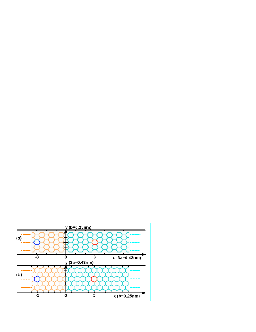
Figure 1: (Color online) A schematic diagram of the graphene PNJ in a armchair ribbon [panel (a)] and in a zigzag ribbon [panel (b)]. The graphene ribbon is along $x$-direction and sharp p-n interface is located at $x=0$. The electron flow injected at $(-L,0)$ [the blue area] in the n-region [orange lattice region] is focused around the symmetric site $(L,0)$ (the red area) in the p-region [green lattice region].

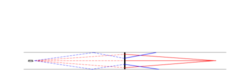
Figure 2: (Color online) After injecting from the source lead in the n-region, the right-going electrons are scattered by the PNJ and boundary of the bipolar graphene ribbon.

In order to study the scattering due to PNJ, we consider two kinds of open bipolar graphene systems (armchair and zigzag ribbons) as shown in Fig.1. The bipolar graphene ribbon consists of semi-infinite electronlike ribbon [orange region] and semi-infinite holelike ribbon [green region] along $x$-direction with a sharp p-n interface located at $x=0$. Electron flow is injected into graphene system from a source lead located at $(-L,0)$ in the n-region. Here we assume that the source lead and the bipolar ribbon are in contact with six lattices [see the blue area in Fig.1]. The injected electrons in the n-region can spread in all directions. Because of the open boundary condition, left-going electrons can finally escape into infinite graphene electrode while right-going electrons [shown in Fig.2] can then be scattered only by p-n interface [thick black line]. Consequently, the response signals are converged around the symmetric site $(L,0)$ [red area in Fig.1]. In order to investigate the focusing current, we couple a detecting electrode locally in the p-region and study the local current (conductance) flowing from that electrode. Clearly, the local current depends on the coupling position of the detecting electrode.

The total Hamiltonian including the infinite graphene ribbon in the tight-binding representationham and the source/drain electrode that is expressed in $k$ space with the free electron model can be written as:

$$H = \sum_{\bf i}\epsilon_{\bf i}a^{\dagger}_{\bf i}a_{\bf i}-\sum_{<{\bf ij}>}te^{i\phi_{\bf ij}}a_{\bf i}^{\dagger}a_{\bf j}$$ (1)

$$+ \sum\limits_{\alpha,k}\left[\epsilon_{\alpha,k}d_{\alpha,k}^{\dagger}d_{{\alpha},k}+(\gamma a_{{\bf i}_{\alpha}}^{\dagger}d_{{\alpha},k}+h.c)\right]$$

where ${\bf i}=({\bf i}_{x},{\bf i}_{y})$ is the index of the discrete site on the honeycomb lattice which is sketched in the Fig.1, and $a_{\bf i}$ and $a_{\bf i}^{\dagger}$ are the annihilation and creation operators at the site ${\bf i}$. Here $\epsilon_{\bf i}$ in the first term of Eq.(1) is the on-site energy (i.e., the energy of the Dirac point) which can be controlled experimentally by the gate voltage. In the n-region or p-region far away from PNJ all the on-site energy are the same with $\epsilon_{{\bf i}}=E_{n}$ or $\epsilon_{{\bf i}}=E_{p}$. Near PNJ, $\epsilon_{\bf i}$ changes from $E_{n}$ to $E_{p}$ abruptly or smoothly for the sharp PNJ or smooth PNJ, respectively. The second term in Eq.(1) is the nearest neighbor hopping term with the hopping energy $t$, ‘$<{\bf ij}>$’ denotes the nearest neighbor lattice sites. When the graphene ribbon is under a uniform perpendicular magnetic field $B_{z}=B$, a phase $\phi_{\bf ij}$ is added in the hopping term, and $\phi_{\bf ij}=\int_{\bf i}^{\bf j}\vec{A}\cdot d\vec{l}/\phi_{0}$ with the vector potential $\vec{A}=(-By,0,0)$ and the flux quanta $\phi_{0}=\hbar/e$. Finally, the last term in Eq.(1) represents the Hamiltonian of the source and detector leads described in the $k$ space and their coupling to the graphene lattices ${\bf i}_{\alpha}$. Here $\alpha=s,d$ represent source and detecting electrodes and $d_{{\alpha},k}$ ($d^{\dagger}_{{\alpha},k}$) is the annihilation (creation) operator of the electrons in the electrode $\alpha$.

When the electron flow is injected from the source electrode into the graphene in the n-region, the response signal is induced everywhere in the p-region. To make a thorough study on the focusing effect, we consider three physical quantities in the p-region: (1) the local current density vector, (2) the local particle density, and (3) the local current (conductance) of the detecting electrode. For quantities (1) and (2), we consider the system without the coupling of the detecting electrode so that the influence of the detecting electrode can be eliminated.

II.1 Local current density vector

The general current density vector $\mathbf{J}_{\mathbf{i}\mathbf{j}}$ from the site ${\bf i}$ to its nearest neighbor site ${\bf j}$ can be expressed as:DOC

$$J_{\mathbf{i}\mathbf{j}} = \frac{e}{h}\int dE~{}~{}\left[{\bf G}^{<}_{\mathbf{i}\mathbf{j}}(E){\bf H}_{\mathbf{j}~{}\mathbf{i}}-{\bf H}_{\mathbf{i}\mathbf{j}}{\bf G}^{<}_{\mathbf{j}~{}\mathbf{i}}(E)\right]$$ (2)

$$= 2\frac{e}{h}{\rm Re}\int dE~{}~{}\left[te^{i\phi_{\bf ji}}{\bf G}^{<}_{\mathbf{i}\mathbf{j}}(E)\right]$$

where $e$ is the electron charge, ${\bf G}^{<}_{\bf ij}$ is the matrix element of the lesser Green’s function of the scattering region. Because the graphene ribbon is translation invariant in the p/n-region, the central scattering region can be chosen arbitrarily as long as the source sites ${\bf i}_{s}$ and the detector sites ${\bf i}_{d}$ are included. From the Keldysh equation, the lesser Green’s function is related to the retarded and advanced Green’s functions,

$${\bf G}^{<}(E)={\bf G}^{r}(E)\left[\sum_{\alpha}{\bf\Sigma}^{<}_{\alpha}(E)\right]{\bf G}^{a}(E)$$ (3)

Here the sum index $\alpha=L,R,s$ denote the left/right graphene lead and source lead with $\alpha\neq d$ because of the decoupling of the detector lead. The retarded Green’s function ${\bf G}^{r}(E)=[{\bf G}^{a}(E)]^{\dagger}=\{E{\bf I}-{\bf H}_{0}-\sum_{\alpha}{\bf\Sigma}^{r}_{\alpha}(E)\}^{-1}$, where ${\bf H}_{0}$ is Hamiltonian matrix of the central scattering region and ${\bf I}$ is the unit matrix with the same dimension as that of ${\bf H}_{0}$, ${\bf\Sigma}_{\alpha}^{r}$ is the retarded self-energy function from the lead-$\alpha$. ${\bf\Sigma}^{r}_{\alpha}$ can be obtained from ${\bf\Sigma}^{r}_{L/R}(E)={\bf H}_{c,L/R}{\bf g}^{r}_{L/R}(E){\bf H}_{L/R,c}$, where ${\bf H}_{c,L/R}$ (${\bf H}_{L/R,c}$) is the coupling from central region (lead-L/R) to lead-L/R (central region) and ${\bf g}^{r}_{L/R}(E)$ is the surface retarded Green’s function of the semi-infinite lead which can be calculated using a transfer matrix method.transfer Concerning the source lead, we take the wide band approximation, then the non-zero elements of self energy matrix ${\bf\Sigma}^{r}_{s}(E)=-i{\bf\Gamma}_{s}/2$ is energy independent, where line-width function ${\bf\Gamma}_{s}=2\pi\gamma^{2}\rho_{s}(E_{F})$. ${\bf\Sigma}^{<}_{\alpha}(E)$ in Eq.(3) is the lesser self energy of the lead-$\alpha$. Because the isolated lead is in the equilibrium, ${\bf\Sigma}^{<}_{\alpha}$ can be obtained from the fluctuation-dissipation theorem:

$${\bf\Sigma}^{<}_{\alpha}(E) = \left[{\bf\Sigma}^{a}_{\alpha}(E)-{\bf\Sigma}^{r}_{\alpha}(E)\right]f_{\alpha}(E)$$ (4)

$$= i{\bf\Gamma}_{\alpha}(E)f_{\alpha}(E)$$

with ${\bf\Sigma}^{a}_{\alpha}={\bf\Sigma}^{r,\dagger}_{\alpha}$ and $f_{\alpha}(E)=f_{0}(E-eV_{\alpha})$ where $f_{0}(E)=1/[{\rm exp}(E/k_{B}\mathcal{T})+1]$ is the Fermi distribution function. $V_{\alpha}$ is the external bias in the terminal-$\alpha$. Since we are interested only in the local response due to the source flow, the external biases are set as $V_{s}=\delta V$ and $V_{L/R}=0$. In calculating transport properties, we divide $G^{<}(E)$ into equilibrium and non-equilibrium parts as

$${\bf G}^{<}(E) = {\bf G}^{r}(E)\left[if_{0}(E)\sum_{\alpha}{\bf\Gamma}_{\alpha}(E)\right]{\bf G}^{a}(E)$$ (5)

$$+ {\bf G}^{r}(E)\left[i\sum_{\alpha}\left\{f_{\alpha}(E)-f_{0}(E)\right\}{\bf\Gamma}_{\alpha}(E)\right]{\bf G}^{a}(E)$$

where the equilibrium term does not contribute to the transport and can be dropped out from now on. It is the non-equilibrium term that gives rise to the system response to the electron injection from the source lead. Because of $V_{s}=\delta V$ and $V_{L/R}=0$, we have

$${\bf G}^{<}(E)=i{\bf G}^{r}(E)\left[f_{s}(E)-f_{0}(E)\right]{\bf\Gamma}_{s}{\bf G}^{a}(E)$$ (6)

Substituting Eq.(6) into Eq.(2) and considering the limit of small source bias, the local current density vector ${\bf J}_{\bf ij}$ (or the local conductance density vector ${\bf J}_{\bf ij}/\delta V$) can be expressed in the following form at zero temperature:

$${\bf J}_{\mathbf{i}\mathbf{j}}/\delta V=\frac{2e}{h}{\rm Im}\left\{te^{i\phi_{\bf ji}}\left[{\bf G}^{r}(E_{F})i{\bf\Gamma}_{s}{\bf G}^{a}(E_{F})\right]_{\bf ij}\right\}$$ (7)

It should be noted that the current density ${\bf J}_{\bf ij}$ in Eq.(7) is defined between the lattice sites ${\bf i}$ and ${\bf j}$ with the direction from site ${\bf i}$ to ${\bf j}$. In order to obtain the local current density vector ${\bf J_{i}}$ at the site ${\bf i}$, we take the weighted average on ${\bf J}_{\bf ij}$ over all the nearest neighbors ${\bf j}$.

II.2 Local particle density

The local particle density (i.e. the electron occupation number) is defined as

$$\rho_{\bf i} = -ie\int\frac{dE}{2\pi}~{}~{}{\bf G}^{<}_{\bf ii}(E)$$ (8)

where ${\bf G}^{<}_{\bf ii}$ is the diagonal element of the lesser Green’s function ${\bf G}^{<}$ in Eq.(3). Similar to the derivation of local current density vector ${\bf J}_{\bf ij}/\delta V$, here we consider only the variation of the local particle density caused by the electron injection from the source lead. At zero temperature and the small bias $\delta V$ limit, substituting Eq.(6) into Eq.(8), the variation of the local particle density is expressed as:

$$\delta\rho_{\bf i}/\delta V \equiv [\rho_{\bf i}(V_{s}=\delta V)-\rho_{\bf i}(V_{s}=0)]/\delta V$$ (9)

$$= \frac{e^{2}}{2\pi}\left[{\bf G}^{r}(E_{F}){\bf\Gamma}_{s}{\bf G}^{a}(E_{F})\right]_{\bf ii}$$

Since the Hamiltonian is defined at discrete lattice sites, the local quantities can also be defined at each lattice site. Such a local quantity is feasible but not necessary. In fact, for graphene, we can define the “local” quantity by averaging over six discrete sites in a unit cell of honeycomb lattice. This average can eliminate the strong variation of local quantities in the A and B sublattices. Now every local site can be determined from the coordinates $(x,y)$ shown in Fig.1. For example, the local injection area displayed in a blue area in Fig.1 is located at $(-3,0)$ in Fig.1(a) and $(-5,0)$ in Fig.1(b). In the whole lattice region in Fig.1, there are $7\times 3$ and $11\times 3$ units in Fig.1(a) and Fig.1(b), respectively.

II.3 Local conductance

Concerning the local conductance, the detecting lead-d is coupled to the graphene ribbon in the p-region. Similar to the local particle density, here the detecting lead also couples to six sites ${\bf i}_{d}$ in a unit cell of honeycomb lattice. The current flowing to the detecting lead-$d$ can be expressed as

$$J_{d} = \frac{e}{\hbar}\sum_{k_{d}}\left[{\bf G}^{<}_{{\bf i}_{d},k_{d}}(t_{1},t_{2}){\bf H}_{k_{d},{\bf i}_{d}}-{\bf H}_{{\bf i}_{d},k_{d}}{\bf G}^{<}_{k_{d},{\bf i}_{d}}(t_{1},t_{2})\right]_{t_{1}=t_{2}}$$ (10)

$$= \frac{e}{\hbar}\sum_{k_{d}}\left]{\bf G}^{<}_{{\bf i}_{d},k_{d}}(t_{1},t_{2})\gamma-\gamma{\bf G}^{<}_{k_{d},{\bf i}_{d}}(t_{1},t_{2})\right]_{t_{1}=t_{2}}$$

Using the Dyson equation in the time contour, we can get the Landauer-B$\ddot{u}$ttiker formulaLanduer which is expressed in terms of non-equilibrium Green’s functions:

$$J_{d} = \frac{e}{\hbar}\sum_{\alpha}\int\frac{dE}{2\pi}{\bf T}_{d,\alpha}(E)[f_{d}(E)-f_{\alpha}(E)].$$ (11)

with $\alpha=L,R,s$ representing the left/right graphene leads and source leads. Since we shall concentrate only on the response current induced by the current injected from the source lead, we use the following boundary conditions $V_{L,R}=V_{d}=0$ and $V_{s}=\delta V$. The current now becomes,

$$J_{d} = \frac{e}{\hbar}\int\frac{dE}{2\pi}[T_{d,s}(E)(f_{d}(E)-f_{s}(E))].$$ (12)

where $T_{d,s}$ is the transmission coefficient from the source lead located at the site ${\bf i}_{s}$ to the detecting lead located at the site ${\bf i}_{d}$ which can be calculated from $T_{d,s}(E)={\rm Tr}\left[{\bf\Gamma}_{d}{\bf G}^{r}(E){\bf\Gamma}_{s}{\bf G}^{a}(E)\right]$, where ${\bf G}^{a}={\bf G}^{r\dagger}$ is the advanced Green’s function in the scattering region. In the wide band limit, the line-width function ${\bf\Gamma}_{s/d}(E)=i({\bf\Sigma}_{s/d}^{r}-{\bf\Sigma}_{s/d}^{r\dagger})=2\pi\gamma^{2}\rho_{s/d}(E_{F})$. Here $f_{s/d}(E)$ in Eq.(12) is the Fermi distribution function of the source and detecting lead, and $f_{s}(E)=f_{0}(E-eV_{s})$ and $f_{d}(E)=f_{0}(E)$. Considering the zero temperature and small bias $V_{s}$ limits, local conductance contributed by the source electron flow can be expressed as:

$$G_{{\bf i}_{d}}=J_{d}/\delta V=\frac{e^{2}}{h}T_{d,s}(E_{F}).$$ (13)

III numerical results and discussion

In the numerical calculations, we set the nearest-neighbor carbon-carbon distance $a=0.142nm$ and the second nearest-neighbor distance $b=\sqrt{3}a\simeq 0.25nm$, the hopping energy $t=2.75eV$ as in a real graphene sample.ref3 In this paper, we consider only the focusing effect of the symmetric PNJ, in which the electron density of n region is the same as the hole density in p region, i.e., $\rho_{e}=\rho_{h}$. For simplicity, we set $E_{F}=0$. Hence in the n-region far away from PNJ the on site energy $\epsilon_{{\bf i}}=E_{n}=-E_{0}$ while $\epsilon_{{\bf i}}=E_{p}=E_{0}$ in the p-region far away from PNJ. Near PNJ, $\epsilon_{\bf i}$ changes from $-E_{0}$ to $E_{0}$ abruptly (smoothly) for the sharp (smooth) PNJ.

Experimentally, it is more convenient to measure the electric conductance. So, in order to detect the focusing effect by a single PNJ in graphene, one can use a small electric contact (such as a STM probe) as a source of electron flow in the n-region and another local probe located in the p-region as a detector. Electric conductance between the two contacts measures the transmission probability for a charged carrier from the source to the detector. Numerically, We have calculated the local conductance $G_{{\bf i}_{d}}$ and confirmed that the distribution of local conductance is similar to that of the local particle density $\delta\rho_{\bf i}/\delta V$. For this reason, only the numerical results on local particle density are shown in this paper. In addition, in order to visualize the focusing process, we also show the distribution of local current density vector in the p-region.

III.1 Focusing effect in very low energy regime

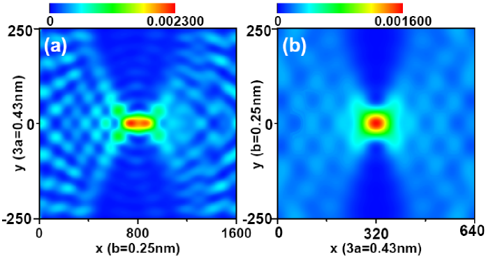
Figure 3: (Color online) Distribution of local particle density $\delta\rho(x,y)/\delta V$ in a graphene ribbon with a single sharp PNJ at $x=0$. Panel (a): zigzag ribbon with ribbon width $W=500\times 3a$. The source flow is injected from the honeycomb unit cell at $(-800b,0)$ and focused around the spot located at $(800b,0)$. Panel (b): the armchair ribbon with ribbon width $W=501b$. The source flow is injected from the honeycomb unit cell at $(-320\times 3a,0)$. The other parameter used: $E_{0}=0.05t$.

Now we study the focusing effect in the graphene ribbon with a sharp PNJ. For a zigzag ribbon or a armchair ribbon with sharp and symmetric PNJ, the spacial distribution of the local particle density $\delta\rho(x,y)/\delta V$ in p-region due to electrons coming from the source lead is shown in Fig.3(a) and Fig.3(b), respectively. Following observations are in order. First of all, electrons injected at $(-L,0)$ in n-region can be focused around $(L,0)$ shown as red spot in Fig.3 which is similar to Ref.[lens, ]. This is because the Fermi energy $E_{F}$ is close to Dirac energy $E_{0}=0.05t$ so that the energy dispersion is nearly linear, i.e., $E_{0}\simeq kb\frac{\sqrt{3}}{2}t$ where $k$ is module of momentum vector $\mathbf{k}$. The charged carriers scattering through PNJ can mimic the refraction of light by left-handed metamaterials with refraction index equal to -1. Secondly, besides the focusing spot (red and green region), there is also a weak interference pattern (blue wave pattern) shown in Fig.3, which is different from Ref.[lens, ] in which the wave pattern is absent. In fact, the wave pattern is solely due to the boundary of the nanoribbon. When an electron is injected from the source area, it can propagate in all directions and the right-going electrons can be scattered by either the boundary of nanoribbon (thin black lines) or sharp PNJ (thick black line) as shown in Fig.2. In the p-region, interference pattern is due to the interference between the state scattered by both boundary and PNJ (thick blue lines) and the state scattered only by PNJ (thick red lines). The spacial period of the interference is proportional to the momentum ${\mathbf{k}}$ or $E_{0}$. Finally, the focusing phenomena in zigzag ribbon is slightly different from that of armchair ribbon: the electron flow is perfectly focused in armchair ribbon [panel (b)], but can’t be fully focused in the zigzag ribbon [panel (a)]. This is because the energy band structures are different for the armchair ribbon and zigzag ribbon. In the following, we will examine the different focusing effects in detail.

III.2 Focusing in zigzag ribbon

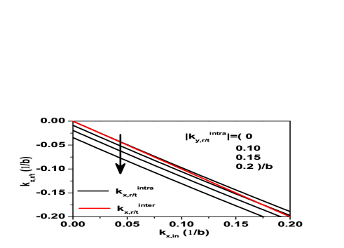
Figure 5: (Color online) Scattering momentum $k_{x,r/t}^{intra}$ and $k_{x,r/t}^{inter}$ vs injecting momentum $k_{x,in}$ for the zigzag ribbon with sharp PNJ. In the interband case, $k_{x,r/t}^{inter}=-k_{x,in}$ for all conserved $k_{y}$ (red line). While in the intraband case (black lines), $k_{x,r/t}^{inter}$ is not equal to $-k_{x,in}$. Different black lines along the black arrow are corresponding to $k_{y}=0$, $0.1/b$, $0.15/b$, $0.2/b$, respectively.

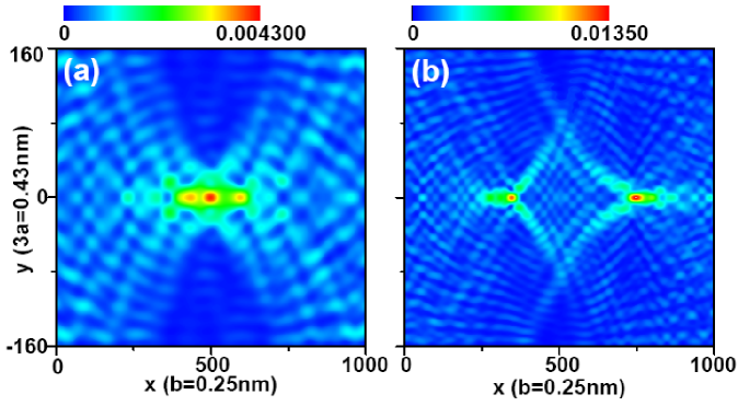
Figure 6: (Color online) Contour of local particle density in zigzag ribbon with a sharp PNJ for $E_{0}=0.1t$ [panel (a)] and $E_{0}=0.2t$ [panel (b)].

When Fermi energy is gradually moved away from Dirac point, the energy spectrum is not ideal conical anymore. In Fig.4 we plot the contour lines of dispersion relation $E(k_{x},k_{y})$ of graphene sheetfootnote with energy interval between nearest contour lines $\delta E=0.1t$. The panel (a) is for the graphene sheet with the carbon-carbon bond along the $x$-direction which corresponds to the armchair graphene ribbon, and the panel (b) is for the graphene sheet with the carbon-carbon bond along the $y$-direction corresponding to the zigzag ribbon. The deviation of ideal conical energy spectrum is clearly exhibited even at small energy $E=0.2t$ (the second small contour lines around the Dirac points $K$ and $K^{\prime}$ show anisotropy behaviors). Since the p-n interface at $x=0$ is along $y$ direction, the $y$ component of momentum, $k_{y}$, is conserved during the scattering. As a result, the incident wave vector $k_{x,in}$, the reflecting wave vector $k_{x,r}$, and the transmitting wave vector $k_{x,t}$ must lie on the black dotted lines in Fig.4. When an electron with energy $E=E_{F}$, velocity $(v_{x},v_{y})$ and corresponding momentum $(k_{x,in},k_{y,in})$ with respect to Dirac point $K$, injects from n-region and is scattered at the p-n interface, according to the identical direction of $V_{x}$, we can solve the reflecting and scattering momentum $k_{x,r}$ and $k_{x,t}$ using the energy conservation and $k_{y}$ conservation. For the zigzag ribbon [corresponding to Fig.4(b)], $k_{x,in}$ can be intra-scattered to $k_{x,r/t}$ around $K$ [$K=(\frac{2}{3}\frac{2\pi}{b},0)$] valley or inter-scattered to $k_{x^{\prime},r/t}$ in $K^{\prime}$ [$K^{\prime}=-(\frac{2}{3}\frac{2\pi}{b},0)$] valley. The interband scattering states is symmetric which satisfies $k^{\prime}_{x,r/t}=-k_{x,in}$. The intraband scattering, however, exhibits asymmetric properties that $\delta k_{x,r/t}\equiv k_{x,in}+k_{x,r/t}\neq 0$ or $v_{x,in}\neq-v_{x,r}$, $v_{x,in}\neq v_{x,t}$ for any fixed $k_{y}$. In Fig.5, we plot the asymmetric relation between $k_{x,in}$ and $k^{intra}_{x,r/t}$ in the intraband scattering and the symmetric relation between $k_{x,in}$ and $k^{inter}_{x,r/t}$ in the interband scattering. We see that in the intraband scattering, the larger $k_{y}$, the larger derivation $\delta k^{intra}_{x,r/t}$ is, while in the interband scattering, $k^{inter}_{x,r/t}$ is always equal to $-k_{x,in}$ for all $k_{y}$. It is known that interband scattering is weakvalleysuppress in pure samples due to the large momentum shift, so the asymmetric intraband scattering is dominant in zigzag ribbon PNJ. As a result, the refraction index can not be strictly equal to $-1$ and the charge flow can’t be fully converged at the symmetric spot. In Fig.6 focusing effect for $E_{0}=0.1t$ and $E_{0}=0.2t$ are plotted, respectively. Comparing Fig.6(a) and Fig.6(b) we see that it is more difficult to focus the electron beam for larger momentum ${\mathbf{k}}$ (energy $E_{0}$).

III.3 Focusing in armchair ribbon

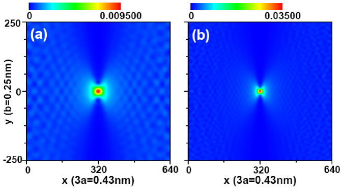
Figure 7: (Color online) Contour of local particle density in armchair ribbon with a sharp PNJ for $E_{0}=0.1t$ [panel (a)] and $E_{0}=0.2t$ [panel (b)].

For the armchair ribbon [corresponding to Fig.4(a)] only intraband scattering occurs. Now $k_{x,in}$ can be symmetrically intra-scattered to $k_{x,r/t}$ in $K$ valley with $-k_{x,in}=k_{x,r}=k_{x,t}$ since $k_{x}$ in Fig.4(a) is symmetric about $k_{x}=0$. So, although the energy dispersion of armchair ribbon is also not strictly linear at high energies as in zigzag ribbon, due to the symmetric scattering, the focusing effect is always perfect in armchair ribbon for all $E_{0}<t$ (i.e. in Dirac fermion regime). Furthermore, with increasing of $E_{0}$, the electron flow coming from n-region shows better convergence in the p-region with smaller focusing spot and stronger intensity. Furthermore, The spacial period of the interference pattern is proportional to the momentum ${\mathbf{k}}$ or $E_{0}$, which can be clearly seen by comparing Fig.3(b), Fig.7(a) and Fig.7(b). .

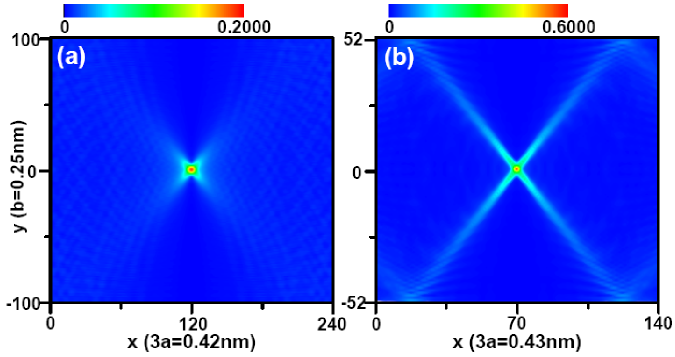
Figure 8: (Color online) Contour of local particle density in armchair ribbon with a sharp PNJ for $E_{0}=0.5t$ [panel (a)] and $E_{0}=0.9t$ [panel (b)].

Roughly speaking, two energy regimes are considered for the Dirac Fermion according to band structure of graphene: (1). ’Near linear dispersion’ regime $0<E_{0}<0.5t$ where $E_{0}\approx kb\frac{\sqrt{3}}{2}t$. (2) ’Beyond linear dispersion’ regime $0.5t<E_{0}<t$ where the energy spectrum is non-conical. The focusing effect corresponding to these two regimes are plotted in Fig.7 and Fig.8, respectively. In the first regime, with the near linear dispersion relation, velocity $v_{x}$ or $v_{y}$ is roughly a constant, and ${k_{y,in}}/{k_{x,in}}\approx{v_{y,in}}/{v_{x,in}}$, ${k_{y,t}}/{k_{x,t}}\approx{v_{y,t}}/{v_{x,t}}$. For the symmetric scattering ($k_{x,in}=k_{x,t}$) in the armchair ribbon, refraction index $n\approx-1$ giving rise to the convergent spot shown in Fig.7. When $E_{0}$ is large enough (larger than 0.5t), energy spectrum is non-conical and velocity now depends on momentum. This leads to a different focusing effect shown in Fig.8 in which crossed focusing zone is present.

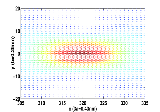
Figure 9: (Color online) Instead of contour of local particle density in Fig.7(b), the quiver of local current density vector around convergence spot is plotted.

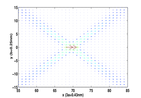
Figure 10: (Color online) Instead of contour of local particle density in Fig.8(b), the quiver of local current density vector around convergence spot is plotted.

In order to show the focusing of the electron flow vividly, instead of the contour of local particle density in Fig.7(b) and Fig.8(b), the quiver of local current density vector around the convergence spot in p-region are plotted in Fig.9 and Fig.10, respectively. For demonstration purpose, the local current density is plotted at every other site. The arrow on each site denotes the local current density vector whose module and direction are described by the size/color and orientation of the arrow respectively. In the low energy regime (Fig.9), the vectors of local current density converge conically to the focusing spot [red spot in Fig.7(b)]. On the other hand, current density is converged mainly from four crossed corners in the high energy regime (Fig.10). Furthermore, comparing Fig.9 and Fig.10, it is clear that electron flow with larger $E_{0}$ gives better convergence.

III.4 Effect of disorders in armchair nanoribbon

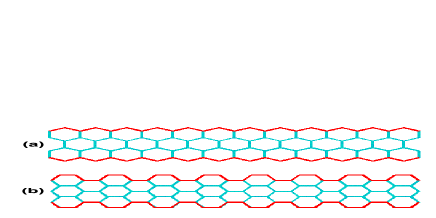
Figure 11: (Color Online) panel (a): sketch of edge in the scattering region with zigzag edge. panel (b) sketch of edge in the scattering region with armchair edge.

As discussed in the previous sections, the clean graphene PNJ is investigated. In a real device, the disorder is always present. In this subsection, we study the disorder effect on the perfect focusing in the armchair nanoribbon. We consider two kinds of disorders, one is induced by random on-site potential $\delta\epsilon_{\bf i}$ and the other is due to the edge defect.edgedefect The random on-site potentials $\delta\epsilon_{\bf i}$ with a uniform distribution $[-w/2,w/2]$ are added near PNJ within the width of $18a$ where $w$ is disorder strength. The edge defect is modeled through missing atoms on the graphene edge. We model the missing atom by setting the corresponding hopping matrix elements to zero. The edge roughness is controlled by $p$, the probability of a missing atom on the outermost row [the red line in Fig.11]. For both on-site potential disorder and edge defect, all data are obtained by averaging over $500$ configurations.

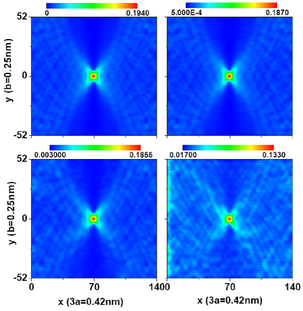
Figure 12: (Color Online) Contour of local particle density in the armchair ribbon with a sharp PNJ for $E_{0}=0.5t$. Panel (a), panel (b), panel (c) and panel (d) are corresponding to random on-site potential strengths $w=0$, $0.2$, $0.5$ and $1.0$, respectively.

In Fig.12 we plot the contour of local particle density in armchair ribbon with a sharp PNJ for $E_{0}=0.5t$ [same as in Fig.8(a)] in the presence of random on-site potential disorder. In Fig.12, the width of armchair ribbon is set to $105b$, the source flow is injected from the honeycomb unit cell at $(-210a,0)$ and focused around the spot located at $(210a,0)$. Panel (a), (b), (c) and (d) correspond to different disorder strengths $w=0$, $0.2$, $0.5$ and $1.0$. For the small random potential strength $w$ (e.g. $w=0.2$), the interference pattern and the focusing spot can be well kept. On the other hand, for the large $w$ (e.g. $w=1.0$), we can see that the random potential disturbs the interference between forward and backward scattering, so the interference pattern is smeared, which increases the density of state outside the focusing spot. Consequently, the intensity of focusing spot decreases. However, we emphasize that although random potential disturbs the interference pattern and reduces the intensity of the focusing spot, the focused spot is clearly visible and its size still remains unchanged. It means that the focusing effect is robust against random potential, especially in the weak disorder case.

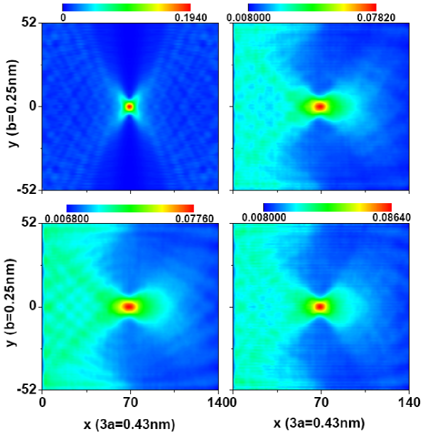
Figure 13: (Color Online) Contour of local particle density in armchair ribbon with a sharp PNJ for $E_{0}=0.5t$. Panel (a), panel (b), panel (c) and panel (d) are corresponding to $p=0$, $0.1$, $0.2$ and $0.5$, respectively.

In Fig.13 we plot the contour of local particle density in the presence of edge defect for $E_{0}=0.5t$. Panel (a), (b), (c) and (d) are corresponding to the different probability $p$ of a missing atom on the outermost row with $p=0$, $0.1$, $0.2$ and $0.5$. We find that in the presence of edge disorder, the size of focusing spot increases clearly and the focusing intensity is greatly reduced. So the effect of the edge defect on the focusing effect is more significant than that of the random potential. But the focusing spot and interference pattern still survive and are clearly visible (see Fig.13d), even in the strong edge defect case with $p=0.5$.

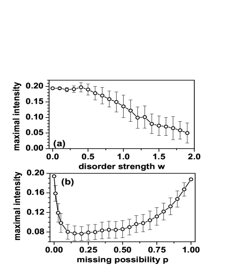
Figure 14: According to Fig.12 and Fig.13, maximum value (the value at the focusing spot central $[L,0]$) of the focusing spot ${\rm LDOS}_{max}$ vs the strength of random potential $w$ [in panel (a)] and probability of one missing atom $p$ [in panel (b)] are plotted, respectively.

To estimate the disorder strength needed to reduce the intensity of focusing spot, in Fig.14(a) and (b), we plot the maximum value (the value at the focusing spot central $[L,0]$) of the focused spot ${\rm LDOS}_{max}$ vs strength of random potential $w$ and the probability of a missing atom $p$. Considering the computational cost, here we take 200 configurations and label the error bar. From Fig.14(a), we find that for weak random potential (when $w<0.5$), ${\rm LDOS}_{max}$ hardly changes with $w$, and focusing effect remains unchanged [see Fig.12(a), (b) and (c)]. Beyond the weak disorder regime ($w>0.5$), ${\rm LDOS}_{max}$ declines abruptly, and focusing effect can’t be kept as good as in the weak disorder regime [see Fig.12(d)]. On the other hand for the edge defect (see Fig.14(b)), we can see that the electron beam can be focused perfectly at $p=0$ and $p=1$ because the graphene ribbon edges are intact at both $p=0$ and $1$. When $p$ increases from $0$ to $1$, more and more atoms in edge are missing until two edges are completely peeled. Correspondingly ${\rm LDOS}_{max}$ decreases first and then increases since the edges are the most random when $p$ is around 0.5. We notice in Fig.14(b), comparing to ${\rm LDOS}_{max}$ near $p=1$, ${\rm LDOS}_{max}$ is reduced faster near $p=0$. It means that the vacancy defect (a few atoms are missing on edges) destroys focusing effect more significantly than the adsorption defect (a few atoms are attached to edges).

III.5 Focusing of armchair ribbon with smooth PNJ

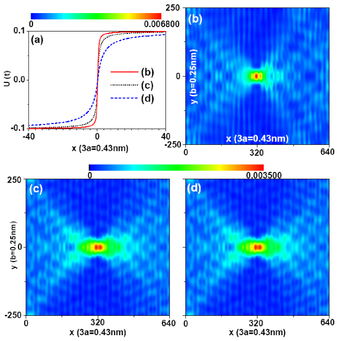
Figure 15: (Color Online) panel (a): smoothly changed $U(x)$ forming smooth PNJ used in panel (b, c, d), in which $x_{0}=0.25*3a$, $0.75*3a$ and $3*3a$, respectively. Panel (b, c, d): Contour of local particle density in armchair ribbon for $E_{0}=0.1$ [same to Fig.7(a) where sharp PNJ is used]. For different panels, smooth PNJ shown in panel (a) are used respectively.

Up to now, we have studied focusing effect by the sharp PNJ. But in realistic graphene based PNJ or PNPJ, the potential changes smoothly from $E_{n}$ to $E_{p}$ within a width $d$. The width $d$ is of the order of the separation between the graphene layer and the top gate and $d\sim~{}$tens nm.pnj In such a smooth PNJ, backscattering is present near PNJ in the distance proportional to $k_{y}$ and interface width $d$, which reduces the possibility of Klein tunneling. For a linear electrostatic potential $U(x)=(vk_{F}/d)x$, the angular dependent transport probabilityKlein $T(\theta)=e^{-\pi(k_{F}d)\sin^{2}(\theta)}$ where $\theta$ is incident angle. It is obvious that the smooth PNJ will reduce the intensity of the focused electron beam due to the decreased transport probability $T(\theta)$. It appears that it also increases the size of the focused spot. Actually, it is not the case due to the following reason. For a single n-p junction (whether smooth or sharp), the electrons (holes) with an energy equal to the chemical potential $\mu=0$ and momentum $k_{x}=k_{F}\cos(\theta)$ transport from conduction (valence) band to the the valence (conduction) band with the conserved $k_{y}=k_{F}\cos(\theta)$ but $k^{\prime}_{x}=-k_{x}$, leading to the almost unchanged focusing pattern, as shown in Fig.15.

The smooth PNJ can be modeled by smoothly varied Dirac energy $U(x)$ across the PNJ. In the numerical calculation, we use the following $U(x)$,

$$U(x)=\left\{\begin{array}[]{rr}-E_{0}\left[1+{{\rm sinh}(\frac{x_{0}}{L})}/{{\rm sinh}(\frac{x-x_{0}}{L})}\right],&x\leq 0\\ &\\ E_{0}\left[1-{{\rm sinh}(\frac{x_{0}}{L})}/{{\rm sinh}(\frac{x+x_{0}}{L})}\right],&x\geq 0\end{array}\right.$$ (17)

where $L$ is the distance between source probe located at $(-L,0)$ and PNJ at $x=0$. In Fig.15(a), with $L=320\times 0.43nm$, $U(x)$ for different $x_{0}$ have been plotted. In Fig.15(b, c, d) with the same parameters used in Fig.7(a) in which the sharp PNJ is used, the contour of local particle density is re-plotted for the smooth PNJ shown in Fig.15(a). We can see that the quantum interference between the states scattered by forward and backward scattering is present. The density of state outside focused spot is increased. Moreover, intensity of the convergent spot is reduced comparing to that of sharp PNJ due to the reduced transmission probability. The wider the PNJ interface, the more the focusing effect is reduced because of the smaller $T(\theta)$. For example, when the PNJ width $d=0$, the maximum of local particle density of state ${\rm LDOS}_{max}=0.0095$ [see Fig.7(a)], increasing $d$ gradually, ${\rm LDOS}_{max}=0.0068$, $0.0035$ [see Fig.15(b) and (c)]. When the PNJ width $d$ is reaching to Fermi wavelength [such that $k_{F}d\sim 1$, in Fig.15, $k_{F}\sim 1/(15a)$], the intensity of focused electron beam decrease very slowly [see Fig.15(c) and (d)]. For the very big $d>>1/k_{F}$, the intensity of focused spot decreases and its size increases continually. In addition, due to the Klein tunneling, the focusing effect can still occur and the convergent contour is almost the same as that of the sharp PNJ, although the intensity of focusing spot is reduced.

III.6 Focusing of armchair ribbon in the presence of small perpendicular magnetic field

In the presence of small perpendicular magnetic field, the momentum $k_{y}$ is not a conserved quantity. In this case, electrons and holes are deflected in opposite directions due to the opposite Lorentz force. So the injecting electron flow in the n-region now can’t be effectively converged in the p-region and the focusing spot is smeared. Considering the opposite deflection for the electrons and holes, the smeared convergent spot will move away from symmetric point $(L,0)$. The larger the size of scattering region, the focusing effect is less significant because of the more deflection in the larger size. On the other hand, the transmission probability $T$ of a single PNJ becomes magnetic field dependent on the field scale $B^{*}=(\hbar/e)k_{F}/d$ with which the cyclotron radius $l_{cycl}=\hbar k_{F}/eB$ becomes comparable to the width $d$ of PNJ. The maximum angle rotating away from normal incidence $\theta_{max}=\pm\arcsin(B/B^{*})$. The transmission probability of a bipolar ribbon is suppressed as $T(B<B^{*})\propto\frac{W}{d}(1-(B/B^{*})^{2})^{3/4}$ where $d$ is width of PNJ and $W$ is width of ribbon.Magnet The influence of transmission probability on focusing effect is mainly to reduce the intensity of focused spot. So in the presence of the weak magnetic field, not only the intensity of focused spot is reduced but the focusing pattern is destroyed by the deflection of electron beam as well.

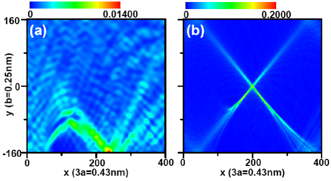
Figure 16: (Color online) Contour of local particle density in the p-region for a armchair ribbon in the perpendicular weak magnetic filed. The sharp PNJ is located at $x=0$. The magnetic field $BS_{0}=0.0001\phi_{0}/\pi$, $E_{0}=0.2t$ in panel (a) and $E_{0}=0.9t$ in panel (b).

In Fig.16, we plot the local particle density in the armchair ribbon with small magnetic field for sharp and symmetric PNJ. For the sharp PNJ, intensity of focused spot is reduced not so severely as in the smooth PNJ. The magnetic field $B$ is expressed in terms of magnetic flux $BS_{0}$ in the unit of $\phi_{0}/\pi$ where $S_{0}=\frac{3}{2}\sqrt{3}a^{2}$ is the area of a honeycomb unit cell and $\phi_{0}=\hbar/e$ is the flux quanta. Here $BS_{0}=0.0001\phi_{0}/\pi$ corresponds to the magnetic field $B=0.4T$. From Fig.16, we can see that in the low energy regime [panel (a), $E_{0}=0.2t$] the focusing effect is destroyed severely, and focusing effect is hardly destroyed in the higher energy regime [panel (b), $E_{0}=0.9t$] due to the less influence of magnetic field on electron flow with higher energy.

IV conclusion

In conclusion, using the tight-binding Hamiltonian, we report the focusing of electron flow in zigzag or armchair graphene ribbon with a single symmetric PNJ. For a sharp PNJ, in the very low energy regime ($|E_{F}-E_{n/p}|=E_{0}<0.05$), graphene ribbon exhibits almost conical energy spectrum and the electron flow coming from n-region can be converged in the p-region perfectly. When energy $E_{0}$ increases, however, energy spectrum gradually deviates from linear behavior. And the band structures are different for zigzag ribbon and armchair ribbon. For the zigzag ribbon, although the interband scattering is symmetric with $-k^{inter}_{x,in}=k^{inter}_{x,r/t}$ but the dominant scattering, intraband scattering, is asymmetric with $k^{intra}_{x,in}+k^{intra}_{x,r/t}\neq 0$. As a result, the electron flow coming from source in n-region can’t be converged in the p-region. As for the armchair ribbon, only the intraband scattering exists which is always symmetric with $-k_{x,in}=k_{x,r/t}$ for all $k_{y}$. This leads to a perfect focusing effect for all energy $E_{0}<t$ regardless of linear or nonlinear dispersion relationship of Dirac Fermion. Specifically, the electron flow converges conically in the low energy regime ($E_{0}<0.5t$), and converge mainly from four crossed corners in the high energy regime ($0.5t<E_{0}<t$). When disorder is present, the perfect focusing in the bipolar ribbon can be robust against disorder induced by the random potential. The perfect focusing is however drastically affected by the edge defect, not only the intensity of focused spot is reduced, the size of spot is also increased. Furthermore, when the real smooth PNJ is considered, Klein tunneling is reduced significantly due to the backscattering. In this case the intensity of convergent spot is reduced, but the convergent contour still remains the same. Finally, small perpendicular magnetic field deflects the electrons and holes in opposite directions, which destroys the perfect focusing effect especially in the low energy regime.

$${\bf ACKNOWLEDGMENTS}$$

We gratefully acknowledge the financial support by a RGC grant (HKU 704308P) from the Government of HKSAR and NSF-China under Grants Nos. 10734110, 10821403, and 10974236.

Figure 4: (Color online) The contour of dispersion relation $E(k_{x},k_{y})$ of graphene sheet. The energy interval between nearest contour lines is $\delta E=0.1t$. Panel (a): $E(k_{x},k_{y})$ of the graphene sheet with the carbon-carbon bond is along the $x$-direction corresponding to armchair ribbon or Fig.LABEL:structure(a). Panel (b): $E(k_{x},k_{y})$ of the graphene sheet with the carbon-carbon bond is along the $y$-direction corresponding to zigzag ribbon or Fig.1(b).

References

- (1) J. C. Slonczewski and P. R. Weiss, Phys. Rev. 109, 272 (1958); G. W. Semenoff, Phys. Rev. Lett. 53, 2449 (1984); F. D. M. Haldane, Phys. Rev. Lett. 61, 2015 (1988).
- (2) A. H. Castro Neto, F.Guinea ,N. M. R. Peres ,K. S. Novselov, and A. K. Geim, Rev. Mod. Phys. 81, 109 (2009);
- (3) K.S. Novoselov, A.K. Geim, S.V. Morozov, D. Jiang, Y. Zhang, S.V. Dubonos, I. V. Grigorieva, and A.A. Firsov, Science 306, 666 (2004).
- (4) K. S. Novoselov, A. K. Geim, S. V. Morozov, D. Jiang, M. I. Katsnelson, I. V. Grigorieva, S. V. Dubonos, and A. A. Firsov, Nature (London) 438, 197 (2005).
- (5) K. Novoselov et al., Nature 438, 197 (2005); Y. Zhang, Y.-W. Tan, H. L. Stormer, P. Kim, Nature 438, 201 (2005); K. Novoselov et al., Nature Phys. 2, 177 (2006); J. R. Williams, L. Dicarlo and C. M. Marcus, Science 317, 638 (2008).
- (6) T. Ohta, A. Bostwick, T. Seyller, K. Horn, E. Rotenberg, Science 313, 951 (2006).
- (7) B. Huard, J. A. Sulpizio, N. Stander, K. Todd, B. Yang, and D. Goldhaber-Gordon, Phys. Rev. Lett. 98, 236803 (2007); A. f. Young and P. Kim, Nature Phys. 5, 222 (2009); B. Özyilmaz, P. Jarillo-Herrero, D. Efetov, D.A. Abanin, L. S. Levitov, and P. Kim, Phys. Rev. Lett. 99, 166804 (2007); J. R. Williams, L. DiCarlo, and C. M. Marcus, Science 317, 638 (2007).
- (8) M. V. Fistul and K. B. Efetov, Phys. Rev. Lett. 98, 256803 (2007).
- (9) A. Ossipov, M. Titov, and C. W. J. Beenakker, Phys. Rev. B 75, 241401(R) (2007).
- (10) S.-G. Cheng, Y. Xing, J. Wang, and Q.-F. Sun, Phys. Rev. Lett. 103, 167003 (2009); Q.-F. Sun and X. C. Xie, J. Phys.: Condens. Matter 21, 344204 (2009).
- (11) M. I. Katsnelson, K. S. Novoselov, and A. K. Geim, Nature Phys. 2, 620 (2006); V. V. Cheianov and V. I. Faĺko, Phys. Rev. B 74 041403(R) (2006).
- (12) A. V. Shytov, M. S. Rudner, and L. S. Levitov, Phys. Rev. Lett. 101, 156804 (2008).
- (13) V. V. Cheianov, V. Faĺko and B. L. Altshuler, Science, 315, 1252 (2007).
- (14) A. F. Young and P. Kim, Nature Phys. 5, 222 (2009).
- (15) J. P. Robinson and H. Schomerus, Phys. Rev. B 76, 115430 (2007); H. Schomerus, Phys. Rev. B 76, 045433 (2007).
- (16) Y. Zhang, Y.-W. Tan, H.L. Stormer, and P. Kim, Nature (London) 438, 201 (2005).
- (17) T. Ando, T. Nakanishi, and R. Saito, J. Phys. Soc. Jpn. 67, 2857 (1998).
- (18) J. B. Pendry, Nature 423, 22 (2003); D. R. Smith, J. B. Pendry, M. Wiltshire, Science 305, 788 (2004).
- (19) J. B. Pendry, Phys. Rev. Lett. 85, 3966 (2000).
- (20) J. Martin, N. Akerman, G. Ulbricht, T. Lohmann, J. H. Smet, K. V. Klitzing and A. Yacoby, Nature Phys. 4, 144 (2008).
- (21) Y. Zhang, V. Brar, C. Girit, A. Zettl and M. F. Crommie, Nature Phys. 5, 722 (2009).
- (22) sec.IV, C. W. J. Beenakker, Mod. Rev. Phys. 80, 1337 (2008).
- (23) D. N. Sheng, L. Sheng, and Z. Y. Weng, Phys. Rev. B 73, 233406 (2006); Z. Qiao and J. Wang, Nanotechnology 18, 435402 (2007); W. Long, Q.-F. Sun, and J. Wang, Phys. Rev. Lett. 101, 166806 (2008); J. Li and S.-Q. Shen, Phys. Rev. B 78, 205308 (2008).
- (24) C. Caroli, R. Combescot, D. Lederer, P. Nozieres and D. Saint-James, J. Phys. C: Dolid St. Phys., bf 4, 2598 (1971); C. Caroli, R. Combescot, P. Nozieres and D. Saint-James, J. Phys. C: Dolid St. Phys., bf 4, 916 (1970).
- (25) D. H. Lee and J. D. Joannopoulos, Phys. Rev. B 23, 4997 (1981); ibid, 23, 4988 (1981).
- (26) Electronic Transport in Mesoscopic Systems, edited by S. Datta (Cambridge University Press, 1995), Chapters. 2 and 3.
- (27) The band structure of a graphene ribbon is same as that of a graphene sheet, except the zigzag edge stateedgestate would be present in ziazag ribbon. However, for the tunneling process beyond the first subband in conducting or valence band, the edge state is not significant, so energy band of garphene sheet can be safely used in graphene ribbon.
- (28) K. Nakada, M. Fujita, G. Dresselhaus and M. S. Dresselhaus, Phys. Rev. B 54, 17954 (1996); K. Wakabayashi, M. Fujita, H. Ajiki and M. Sigrist, Phys. Rev. B 59, 8271 (1999).
- (29) A. F. Morpurgo, F. Guinea, Phys. Rev. Lett. 97, 196804 (2006); S. V. Morozov, K. S. Novoselov, M. I. Katsnelson, F. Schedin, L. A. Ponomarenko, D. Jiang, and A. K. Geim, Phys. Rev. Lett. 97, 016801 (2006); E. McCann, K. Kechedzhi, Vladimir I. Fal ko, H. Suzuura, T. Ando, and B. L. Altshuler, Phys. Rev. Lett. 97, 146805 (2006).
- (30) M. Evaldsson, I. V. Zozoulenko, Hengyi Xu, and T. Heinzel, Phys. Rev. B 78, 161407(R) (2008); Hengyi Xu and T. Heinzel, I. V. Zozoulenko, Phys. Rev. B 80, 045308 (2009).
- (31) A. V. Shytov, Nan Gu, L. S. Levitov, cond-mat/0708.3081 (2007).