The $P$-wave $[cs][\bar{c}\bar{s}]$ tetraquark state: $Y(4260)$ or $Y(4660)$?

Abstract

The mass of $P$-wave $cs$-scalar-diquark $\bar{c}\bar{s}$-scalar-antidiquark state is computed in the framework of QCD sum rules. The result $4.69\pm 0.36~{}\mbox{GeV}$ is in good agreement with the experimental value of $Y(4660)$ but higher than $Y(4260)$’s, which supports the $P$-wave $[cs][\bar{c}\bar{s}]$ configuration for $Y(4660)$ while disfavors the interpretation of $Y(4260)$ as the $P$-wave $[cs][\bar{c}\bar{s}]$ state. In the same picture, the mass of $P$-wave $[bs][\bar{b}\bar{s}]$ is predicted to be $11.19\pm 0.49~{}\mbox{GeV}$.

I Introduction

Fruitful heavy hadrons have been observed by far, some of which attribute to the $J^{PC}=1^{--}$ family, e.g. $Y(4260)$, $Y(4360)$, and $Y(4660)$. The observation of $Y(4260)$ was first announced by BABAR Collaboration Y4260-BABAR , which was confirmed later by both CLEO Collaboration Y4260-CLEO and Belle Collaboration Y4260-Belle . A fit to the resonance yields a mass $4263^{+8}_{-9}~{}\mbox{MeV}$ PDG . Subsequently, $Y(4360)$ Y4325 ; Y4360-fit ; Y4360 and $Y(4660)$ Y4360 were reported by BaBar Collaboration and Belle Collaboration, masses of which are $4361\pm 9\pm 9~{}\mbox{MeV}$ and $4664\pm 11\pm 5~{}\mbox{MeV}$, respectively. Since then, these states have inspired intensive theoretical speculations. Concretely, $Y(4260)$ is proposed as a hybrid charmonium Y4260 , a $\chi_{c}\rho^{0}$ molecular state Y4260-Liu , a conventional $\Psi(4S)$ Y4260-FJ , an $\omega\chi_{c1}$ molecular state Y4260-Yuan , a $\Lambda_{c}\bar{\Lambda}_{c}$ baryonium state Y4260-Qiao , and a $D_{1}D$ or $D_{0}D^{*}$ hadronic molecule Y4260-Ding ; $Y(4360)$ is interpreted as the candidate of the charmonium hybrid or a $3^{3}D_{1}$ $c\bar{c}$ state Ding ; $Y(4660)$ is suggested to be a $5^{3}S_{1}$ charmonium Ding , a baryonium state Qiao ; Y4660-Bugg , a $f_{0}(980)\Psi^{\prime}$ bound state Guo ; zgwang , a $6^{3}S_{1}$ state KTChao , and a $5^{3}S_{1}-4^{3}D_{1}$ mixing state Badalian . Besides, many other renewed works renewed have appeared continually.

In the tetraquark picture, $Y(4260)$ is deciphered as the $P$-wave $[cs][\bar{c}\bar{s}]$ state Y4260-L (named as $Y_{[cs]}$ here), however, some authors do not go along with the assumption and figure that $Y(4260)$ cannot be a $P$-wave charm-strange diquark-antidiquark Y4660-Ebert . Otherwise, some researchers study $Y(4660)$ as a charm-strange tetraquark state Y4660-QCDSR . Under such a circumstance, it is interesting and necessary to make clear whether $Y(4260)$ can be interpreted as the $P$-wave $[cs][\bar{c}\bar{s}]$ state or $Y(4660)$ can be a candidate of the $Y_{[cs]}$. Indubitably, the quantitative investigation of $Y_{[cs]}$’s mass is very instructive for comprehending its structure, but it is quite difficult to extract hadronic spectrum information from the QCD basic theory. Fortunately, one can make use of QCD sum rules svzsum (for reviews see overview ; overview1 ; overview2 ; overview3 and references therein), which is entrenched in the QCD first principle. Just in this work, we devote to reckon the mass of $Y_{[cs]}$ through the QCD sum rule, to study whether $Y(4260)$ or $Y(4660)$ can be a $P$-wave $[cs][\bar{c}\bar{s}]$ state. In addition, $Y_{b}(10890)$ Y10890 ; Y10890-new has been interpreted as a $P$-wave $[bq][\bar{b}\bar{q}]$ tetraquark state tetraquark . Similarly, the bottom counterpart $[bs][\bar{b}\bar{s}]$ for $Y_{[cs]}$ could exist, thereby $Y_{[bs]}$’s mass is also predicted here.

The paper is planned as follows. The QCD sum rule for the tetraquark state is introduced in Sec. II, and both the phenomenological and QCD side are derived, followed by the numerical analysis and some discussions in Sec. III. Section IV is a brief summary.

II the $P$-wave $[Qs][\bar{Q}\bar{s}]$ QCD sum rule

The QCD sum rule bridges the gap between the hadron phenomenology and the quark-gluon interactions. By analogy with the structure of $P$-wave $[Qq][\bar{Q}\bar{q}]$ in Ref. diquark , the $Y_{[Qs]}$ is a $J^{PC}=1^{--}$ bound diquark-antidiquark state having the flavor content $Y_{[Qs]}=[Qs][\bar{Q}\bar{s}]$ with the spin and orbital momentum numbers: $S_{[Qs]}=0$, $S_{[\bar{Q}\bar{s}]}=0$, $S_{[Qs][\bar{Q}\bar{s}]}=0$, and $L_{[Qs][\bar{Q}\bar{s}]}=1$. For the interpolating current, a derivative could be included in order to generate $L_{[Qs][\bar{Q}\bar{s}]}=1$. Presently, one constructs the tetraquark state current from diquark-antidiquark configuration of fields, while constructs the molecular state current from meson-meson type of fields. While these two types of currents can be related to each other by Fiertz rearrangements, the relations are suppressed by a typical color and Dirac factor so that one could obtain a reliable sum rule only if one has chosen the appropriate current to have a maximum overlap with the physical state (on this point, there are some calculations and discussions in the XII. Appendix in Ref. overview-MN ). Concretely, it will have a maximum overlap for the tetraqurk state using the diquark-antidiquark current and the sum rule can reproduce the physical mass well, whereas the overlap for the tetraqurk state employing a meson-meson type of current will be small and the sum rule will not be able to reproduce the mass well. Thus, the following form of current could be constructed for $Y_{[Qs]}$,

$$j^{\mu}=\epsilon_{abc}\epsilon_{dec}(s_{a}^{T}C\gamma_{5}Q_{b})D^{\mu}(\bar{s}_{d}\gamma_{5}C\bar{Q}_{e}^{T}).$$ (1)

Here the index $T$ means matrix transposition, $C$ is the charge conjugation matrix, $D^{\mu}$ denotes the covariant derivative, as well as $a$, $b$, $c$, $d$, and $e$ are color indices.

To derive the mass sum rule, one starts from the two-point correlator

$$\Pi^{\mu\nu}(q^{2})=i\int d^{4}x\mbox{e}^{iq.x}\langle 0|T[j^{\mu}(x)j^{\nu+}(0)]|0\rangle.$$ (2)

Lorentz covariance implies that the two-point correlator can be generally parameterized as

$$\Pi^{\mu\nu}(q^{2})=(\frac{q^{\mu}q^{\nu}}{q^{2}}-g^{\mu\nu})\Pi^{(1)}(q^{2})+\frac{q^{\mu}q^{\nu}}{q^{2}}\Pi^{(0)}(q^{2}).$$ (3)

The part of the correlator proportional to $g_{\mu\nu}$ is chosen to attain the sum rule here. Phenomenologically, $\Pi^{(1)}(q^{2})$ can be expressed as

$$\Pi^{(1)}(q^{2})=\frac{[\lambda^{(1)}]^{2}}{M_{H}^{2}-q^{2}}+\frac{1}{\pi}\int_{s_{0}}^{\infty}ds\frac{\mbox{Im}\Pi^{(1)\mbox{phen}}(s)}{s-q^{2}}+\mbox{subtractions},$$ (4)

where $M_{H}$ denotes the mass of the hadronic resonance. In the OPE side, $\Pi^{(1)}(q^{2})$ can be written as

$$\Pi^{(1)}(q^{2})=\int_{(2m_{Q}+2m_{s})^{2}}^{\infty}ds\frac{\rho^{\mbox{OPE}}(s)}{s-q^{2}},$$ (5)

where the spectral density is given by $\rho^{\mbox{OPE}}(s)=\frac{1}{\pi}\mbox{Im}\Pi^{\mbox{(1)}}(s)$. After equating the two sides, assuming quark-hadron duality, and making a Borel transform, the sum rule can be written as

$$[\lambda^{(1)}]^{2}e^{-M_{H}^{2}/M^{2}} = \int_{(2m_{Q}+2m_{s})^{2}}^{s_{0}}ds\rho^{\mbox{OPE}}(s)e^{-s/M^{2}}.$$ (6)

Eliminating the hadronic coupling constant $\lambda^{(1)}$, one could yield

$$M_{H}^{2} = \int_{(2m_{Q}+2m_{s})^{2}}^{s_{0}}ds\rho^{\mbox{OPE}}se^{-s/M^{2}}/\int_{(2m_{Q}+2m_{s})^{2}}^{s_{0}}ds\rho^{\mbox{OPE}}e^{-s/M^{2}}.$$ (7)

For the OPE calculations, one works at leading order in $\alpha_{s}$ and considers condensates up to dimension six, with the similar techniques developed in technique ; technique1 . The $s$ quark is dealt as a light one and the diagrams are considered up to the order $m_{s}$. To keep the heavy-quark mass finite, one uses the momentum-space expression for the heavy-quark propagator, and the expressions with two and three gluons attached reinders are used. The light-quark part of the correlation function is calculated in the coordinate space and then Fourier-transformed to the momentum space in $D$ dimension. The resulting light-quark part is combined with the heavy-quark part before it is dimensionally regularized at $D=4$. Finally with

$$\rho^{\mbox{OPE}}(s) = \rho^{\mbox{pert}}(s)+\rho^{\langle\bar{s}s\rangle}(s)+\rho^{\langle\bar{s}s\rangle^{2}}(s)+\rho^{\langle g\bar{s}\sigma\cdot Gs\rangle}(s)+\rho^{\langle g^{2}G^{2}\rangle}(s)+\rho^{\langle g^{3}G^{3}\rangle}(s),$$

$$\rho^{\mbox{pert}}(s) = -\frac{1}{3\cdot 5\cdot 2^{11}\pi^{6}}\int_{\alpha_{min}}^{\alpha_{max}}\frac{d\alpha}{\alpha^{4}}\int_{\beta_{min}}^{1-\alpha}\frac{d\beta}{\beta^{4}}(1-\alpha-\beta)K(\alpha,\beta)[r(m_{Q},s)-5m_{Q}m_{s}]r(m_{Q},s)^{4},$$

$$\rho^{\langle\bar{s}s\rangle}(s) = \frac{\langle\bar{s}s\rangle}{3\cdot 2^{6}\pi^{4}}\{\int_{\alpha_{min}}^{\alpha_{max}}\frac{d\alpha}{\alpha^{2}}\int_{\beta_{min}}^{1-\alpha}\frac{d\beta}{\beta^{2}}\{[(2-\alpha-\beta)m_{Q}+(1-\alpha-\beta)m_{s}]r(m_{Q},s)$$

$${}-3(\alpha-\alpha^{2}+\beta-\beta^{2})m_{s}m_{Q}^{2}\}r(m_{Q},s)^{2}-m_{s}\int_{\alpha_{min}}^{\alpha_{max}}\frac{d\alpha}{\alpha(1-\alpha)}[m_{Q}^{2}-\alpha(1-\alpha)s]^{3}\},$$

$$\rho^{\langle\bar{s}s\rangle^{2}}(s) = \frac{m_{Q}\langle\bar{s}s\rangle^{2}}{3\cdot 2^{4}\pi^{2}}\int_{\alpha_{min}}^{\alpha_{max}}d\alpha\{-2m_{Q}[m_{Q}^{2}-\alpha(1-\alpha)s]+m_{s}[m_{Q}^{2}-2\alpha(1-\alpha)s]\},$$

$$\rho^{\langle g\bar{s}\sigma\cdot Gs\rangle}(s) = \frac{\langle g\bar{s}\sigma\cdot Gs\rangle}{3\cdot 2^{8}\pi^{4}}\{\int_{\alpha_{min}}^{\alpha_{max}}\frac{d\alpha}{\alpha^{2}}\int_{\beta_{min}}^{1-\alpha}\frac{d\beta}{\beta^{2}}r(m_{Q},s)\{-3m_{Q}(\alpha+\beta-4\alpha\beta)r(m_{Q},s)$$

$${}+m_{s}\alpha\beta[12m_{Q}^{2}-7(\alpha+\beta)m_{Q}^{2}-5\alpha\beta s]\}$$

$${}+\int_{\alpha_{min}}^{\alpha_{max}}d\alpha[m_{Q}^{2}-\alpha(1-\alpha)]\{\frac{3m_{Q}}{\alpha(1-\alpha)}[m_{Q}^{2}-\alpha(1-\alpha)s]+2m_{s}[5\alpha(1-\alpha)s-9m_{Q}^{2}]\}\},$$

$$\rho^{\langle g^{2}G^{2}\rangle}(s) = -\frac{m_{Q}\langle g^{2}G^{2}\rangle}{3^{2}\cdot 2^{12}\pi^{6}}\int_{\alpha_{min}}^{\alpha_{max}}\frac{d\alpha}{\alpha^{4}}\int_{\beta_{min}}^{1-\alpha}\frac{d\beta}{\beta^{4}}(1-\alpha-\beta)(\alpha^{3}+\beta^{3})K(\alpha,\beta)r(m_{Q},s)$$

$${}\times[(m_{Q}-3m_{s})r(m_{Q},s)-2m_{s}m_{Q}^{2}(\alpha+\beta)],~{}\mbox{and}$$

$$\rho^{\langle g^{3}G^{3}\rangle}(s) = -\frac{\langle g^{3}G^{3}\rangle}{3^{2}\cdot 2^{14}\pi^{6}}\int_{\alpha_{min}}^{\alpha_{max}}\frac{d\alpha}{\alpha^{4}}\int_{\beta_{min}}^{1-\alpha}\frac{d\beta}{\beta^{4}}(1-\alpha-\beta)K(\alpha,\beta)\{[(\alpha^{3}+\beta^{3})r(m_{Q},s)+4(\alpha^{4}+\beta^{4})m_{Q}^{2}$$

$${}-2m_{Q}m_{s}(2\alpha^{2}+3\alpha\beta+2\beta^{2})(3\alpha^{2}-4\alpha\beta+3\beta^{2})]r(m_{Q},s)-4m_{s}m_{Q}^{3}(\alpha+\beta)(\alpha^{4}+\beta^{4})\}.$$

It is defined as $r(m_{Q},s)=(\alpha+\beta)m_{Q}^{2}-\alpha\beta s$ and $K(\alpha,\beta)=1+\alpha-2\alpha^{2}+\beta+2\alpha\beta-2\beta^{2}$. The integration limits are given by $\alpha_{min}=(1-\sqrt{1-4m_{Q}^{2}/s})/2$, $\alpha_{max}=(1+\sqrt{1-4m_{Q}^{2}/s})/2$, and $\beta_{min}=\alpha m_{Q}^{2}/(s\alpha-m_{Q}^{2})$.

III Numerical analysis and discussions

In this section, the sum rule (7) will be numerically simulated. The input parameters are taken as $\langle\bar{q}q\rangle=-(0.23\pm 0.03)^{3}~{}\mbox{GeV}^{3}$, $\langle\bar{s}s\rangle=0.8~{}\langle\bar{q}q\rangle$, $\langle g\bar{s}\sigma\cdot Gs\rangle=m_{0}^{2}~{}\langle\bar{s}s\rangle$, $m_{0}^{2}=0.8~{}\mbox{GeV}^{2}$, $\langle g^{2}G^{2}\rangle=0.88~{}\mbox{GeV}^{4}$, and $\langle g^{3}G^{3}\rangle=0.045~{}\mbox{GeV}^{6}$ overview2 ; Y4660-QCDSR ; parameters . For the quark masses, we employ the same values as Ref. Narison and references therein, which spanned by the running $\overline{MS}$ mass and the on-shell mass from QCD sum rule, with $m_{c}=1.26\sim 1.47~{}\mbox{GeV}$, $m_{b}=4.22\sim 4.72~{}\mbox{GeV}$, as well as $m_{s}=114.5\pm 20.8~{}\mbox{MeV}$. Complying with the standard criterion of sum rule analysis, the threshold $s_{0}$ and Borel parameter $M^{2}$ are varied to find the stability window. It is well known that the fundamental assumption of the QCD sum rule is the principle of duality: it is assumed that there is an interval over which a hadron may be equivalently described at both the quark level and the hadron level. Therefore, the correlation function is evaluated in two different ways: at the quark level in terms of quark and gluon fields and at the hadronic level. If both sides of the sum rule were calculated to arbitrarily high accuracy, the matching of them would be independent of $M^{2}$. Practically, however, both sides are represented imperfectly. On one hand, there are approximations in the OPE of the correlation functions and, on the other hand, there is a very complicated and largely unknown structure of the hadronic dispersion integrals in the phenomenological side. Thus, the extracted result is not completely independent of $M^{2}$. The hope is that there exists a range of $M^{2}$, in which the two sides have a good overlap and information on the resonance can be extracted. In practice, one can analyse the OPE convergence and the pole contribution to determine the allowed Borel window of $M^{2}$: the lower limit constraint for $M^{2}$ is obtained by restricting that the perturbative contribution should be larger than the condensate contributions; the upper limit constraint is gained by the consideration that the pole contribution should be larger than QCD continuum contribution. Meanwhile, the threshold parameter $\sqrt{s_{0}}$ characterizes the beginning of the continuum state. Thereby, it is not arbitrary but correlated to the energy of the next excited state with the same quantum number as the studied state.

At first, we keep the values of the quark masses and condensates fixed at the central values. The comparison between pole and continuum contributions from sum rule (6) for $Y_{[cs]}$ for $\sqrt{s_{0}}=5.2~{}\mbox{GeV}$ is shown in the left part of FIG. 1, and its OPE convergence by comparing the perturbative, quark condensate, four-quark condensate, mixed condensate, two-gluon condensate, and three-gluon condensate contributions is shown in the right one. Numerically, the ratio of perturbative contribution to the total OPE contribution at $M^{2}=2.5~{}\mbox{GeV}^{2}$ is nearly $60\%$, which is increasing with the $M^{2}$ to insure that perturbative contribution can dominate in the total OPE contribution when $M^{2}\geq 2.5~{}\mbox{GeV}^{2}$. On the other side, the relative pole contribution is approximate to $52\%$ at $M^{2}=3.2~{}\mbox{GeV}^{2}$ and descending along with the $M^{2}$ to guarantee the pole contribution can dominate in the total contribution while $M^{2}\leq 3.2~{}\mbox{GeV}^{2}$. Thus, the region of $M^{2}$ for $Y_{[cs]}$ is taken as $M^{2}=2.5\sim 3.6~{}\mbox{GeV}^{2}$ for $\sqrt{s_{0}}=5.2~{}\mbox{GeV}$. Similarly, the proper range of $M^{2}$ is gained as $2.5\sim 3.0~{}\mbox{GeV}^{2}$ for $\sqrt{s_{0}}=5.0~{}\mbox{GeV}$, and the range of $M^{2}$ is $2.5\sim 3.6~{}\mbox{GeV}^{2}$ for $\sqrt{s_{0}}=5.4~{}\mbox{GeV}$. We see also that for $\sqrt{s_{0}}=4.9~{}\mbox{GeV}$, the corresponding Borel parameter range is $M^{2}=2.5\sim 2.7~{}\mbox{GeV}^{2}$, which is very narrow as a working window. It is the main reason that $\sqrt{s_{0}}\leq 4.9~{}\mbox{GeV}$ is not chosen here. In order to evaluate the uncertainty of results more conservatively FESR , we enlarge the variation of threshold parameter $\sqrt{s_{0}}$ for $Y_{cs}$ from $5.0\sim 5.4~{}\mbox{GeV}$ to $5.0\sim 5.7~{}\mbox{GeV}$ and we find the range of $M^{2}$ is $2.5\sim 3.8~{}\mbox{GeV}^{2}$ for $\sqrt{s_{0}}=5.7~{}\mbox{GeV}$. In the chosen region, the mass result is not completely independent of $M^{2}$ since both sides of the sum rule are not calculated to arbitrarily high accuracy but have included some approximations, and that is just the reason by which the accuracy of QCD sum rule method is limited. Whereas, it is expected that the two sides have a good overlap and information on the resonance can be safely extracted in the chosen range of $M^{2}$. The corresponding Borel curve to determine the mass of $Y_{[cs]}$ is exhibited in the left part of FIG. 3. We compute the average mass value of these working windows as $4.69\pm 0.29~{}\mbox{GeV}$ (the numerical error reflects the uncertainty due to variation of $s_{0}$ and $M^{2}$). Up to now, we have kept the values of the quark masses and condensates at the central values. At last, we vary the quark masses as well as condensates and arrive at $4.69\pm 0.29\pm 0.07~{}\mbox{GeV}$ (the first error reflects the uncertainty due to variation of $s_{0}$ and $M^{2}$, and the second error resulted from the variation of QCD parameters) or $4.69\pm 0.36~{}\mbox{GeV}$ in a concise form.

For $Y_{[bs]}$, the comparison between pole and continuum contributions from sum rule (6) for $\sqrt{s_{0}}=11.8~{}\mbox{GeV}$ is shown in the left part of FIG. 2, and its OPE convergence by comparing different OPE contributions is shown in the right one. In detail, the perturbative contribution versus the total OPE contribution at $M^{2}=7.5~{}\mbox{GeV}^{2}$ is nearly $62\%$, and the relative pole contribution is approximate to $50\%$ at $M^{2}=9.0~{}\mbox{GeV}^{2}$. Thus, the region of $M^{2}$ is taken as $M^{2}=7.5\sim 9.0~{}\mbox{GeV}^{2}$ for $\sqrt{s_{0}}=11.8~{}\mbox{GeV}$. With the similar analysis, for $\sqrt{s_{0}}=11.6~{}\mbox{GeV}$, the range is $M^{2}=7.5\sim 8.3~{}\mbox{GeV}^{2}$; for $\sqrt{s_{0}}=12.0~{}\mbox{GeV}$, the range is $M^{2}=7.5\sim 9.5~{}\mbox{GeV}^{2}$. To evaluate the uncertainty of results more conservatively, we enlarge the variation of $\sqrt{s_{0}}$ from $11.6\sim 12.0~{}\mbox{GeV}$ to $11.6\sim 12.3~{}\mbox{GeV}$. For $\sqrt{s_{0}}=12.3~{}\mbox{GeV}$, the range of $M^{2}$ is $7.5\sim 10.3~{}\mbox{GeV}^{2}$. The dependence on $M^{2}$ for the mass of $Y_{[bs]}$ from sum rule (7) is shown in the right part of FIG. 3. For $Y_{bs}$, We arrive at $11.19\pm 0.28~{}\mbox{GeV}$ (not including the variation of QCD parameters). Finally, we vary the quark masses as well as condensates and arrive at $11.19\pm 0.28\pm 0.21~{}\mbox{GeV}$ (the former error reflects the uncertainty due to variation of $s_{0}$ and $M^{2}$, and the latter error resulted from the variation of QCD parameters) or $11.19\pm 0.49~{}\mbox{GeV}$ in a concise form.

With regard to the numerical results, some more discussions are given below. Numerically, the result $4.69\pm 0.36~{}\mbox{GeV}$ for $Y_{[cs]}$ is in good agreement with the experimental value $4664\pm 11\pm 5~{}\mbox{MeV}$ for $Y(4660)$. However, its value is a bit higher than $Y(4260)$’s mass even considering the uncertainty, which supports the $P$-wave $[cs][\bar{c}\bar{s}]$ structure for $Y(4660)$ while disfavors the explanation of $Y(4260)$ as the $P$-wave $[cs][\bar{c}\bar{s}]$ state. Note that some authors also assume that $Y(4260)$ could be a $P$-wave $[cq][\bar{c}\bar{q}]$ state Y4660-Ebert . In fact, we have calculated the mass of the $P$-wave $[cq][\bar{c}\bar{q}]$ to be $4.32\pm 0.20~{}\mbox{GeV}$ jrz , which is compatible with the experimental data of $Y(4360)$ and could support $Y(4360)$’s $P$-wave $[cq][\bar{c}\bar{q}]$ structure. Barely from the value $4.32\pm 0.20~{}\mbox{GeV}$, one could not completely exclude the possibility of $Y(4260)$ as a $P$-wave $[cq][\bar{c}\bar{q}]$ state since it is still in accord with the mass of $Y(4260)$ in view of the uncertainty. Concerning the real nature of $Y(4260)$, some further theoretical study and experimental verification are undoubtedly needed.

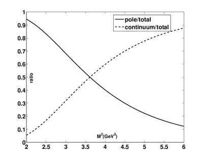
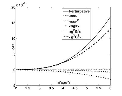
Figure 1: In the left part, the solid line shows the relative pole contribution (the pole contribution divided by the total, pole plus continuum contribution) and the dashed line shows the relative continuum contribution from sum rule (6) for $\sqrt{s_{0}}=5.2~{}\mbox{GeV}$ for $Y_{[cs]}$. The OPE convergence is shown by comparing the perturbative, quark condensate, four-quark condensate, mixed condensate, two-gluon condensate and three-gluon condensate contributions from sum rule (6) for $\sqrt{s_{0}}=5.2~{}\mbox{GeV}$ for $Y_{[cs]}$ in the right one.

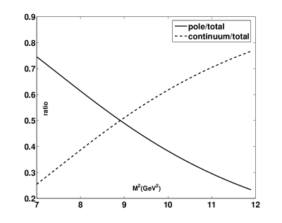
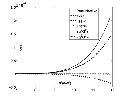
Figure 2: In the left part, the solid line shows the relative pole contribution (the pole contribution divided by the total, pole plus continuum contribution) and the dashed line shows the relative continuum contribution from sum rule (6) for $\sqrt{s_{0}}=11.8~{}\mbox{GeV}$ for $Y_{[bs]}$. The OPE convergence is shown by comparing the perturbative, quark condensate, four-quark condensate, mixed condensate, two-gluon condensate and three-gluon condensate contributions from sum rule (6) for $\sqrt{s_{0}}=11.8~{}\mbox{GeV}$ for $Y_{[bs]}$ in the right one.

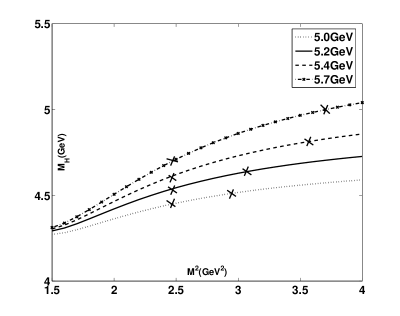
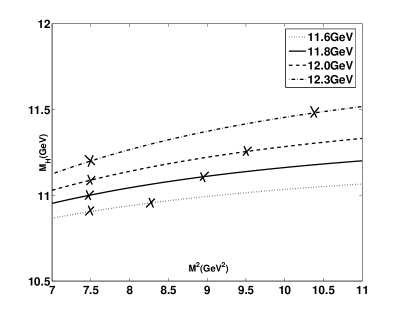
Figure 3: In the left part, the dependence on $M^{2}$ for the mass of $Y_{[cs]}$ from sum rule (7) is shown. The continuum thresholds are taken as $\sqrt{s_{0}}=5.0\sim 5.7~{}\mbox{GeV}$. For $\sqrt{s_{0}}=5.0~{}\mbox{GeV}$, the range of $M^{2}$ is $2.5\sim 3.0~{}\mbox{GeV}^{2}$; for $\sqrt{s_{0}}=5.2~{}\mbox{GeV}$, the range of $M^{2}$ is $2.5\sim 3.2~{}\mbox{GeV}^{2}$; for $\sqrt{s_{0}}=5.4~{}\mbox{GeV}$, the range of $M^{2}$ is $2.5\sim 3.6~{}\mbox{GeV}^{2}$; for $\sqrt{s_{0}}=5.7~{}\mbox{GeV}$, the range of $M^{2}$ is $2.5\sim 3.8~{}\mbox{GeV}^{2}$. The dependence on $M^{2}$ for the mass of $Y_{[bs]}$ from sum rule (7) is shown in the right one. The continuum thresholds are taken as $\sqrt{s_{0}}=11.6\sim 12.3~{}\mbox{GeV}$. For $\sqrt{s_{0}}=11.6~{}\mbox{GeV}$, the ranges of $M^{2}$ is $7.5\sim 8.3~{}\mbox{GeV}^{2}$; for $\sqrt{s_{0}}=11.8~{}\mbox{GeV}$, the range of $M^{2}$ is $7.5\sim 9.0~{}\mbox{GeV}^{2}$; for $\sqrt{s_{0}}=12.0~{}\mbox{GeV}$, the range of $M^{2}$ is $7.5\sim 9.5~{}\mbox{GeV}^{2}$; for $\sqrt{s_{0}}=12.3~{}\mbox{GeV}$, the range of $M^{2}$ is $7.5\sim 10.3~{}\mbox{GeV}^{2}$.

IV Summary

The QCD sum rule method has been employed to compute the mass of $P$-wave $[cs][\bar{c}\bar{s}]$ tetraquark state $Y_{[cs]}$, including contributions of operators up to dimension six in the OPE. The final result $4.69\pm 0.36~{}\mbox{GeV}$ ($4.69\pm 0.29\pm 0.07~{}\mbox{GeV}$, where the first error reflects the uncertainty due to variation of $s_{0}$ and $M^{2}$, and the second error resulted from the variation of QCD parameters) for $Y_{[cs]}$ is well compatible with the experimental data of $Y(4660)$, which favors the $P$-wave tetraquark configuration for $Y(4660)$. Meanwhile, the result is higher than $Y(4260)$’s mass, which is not consistent with assumption of $Y(4260)$ as the $P$-wave $[cs][\bar{c}\bar{s}]$ state. As a byproduct, the mass for the bottom counterpart $Y_{[bs]}$ has also been predicted, which is $11.19\pm 0.49~{}\mbox{GeV}$ ($11.19\pm 0.28\pm 0.21~{}\mbox{GeV}$, where the former error reflects the uncertainty due to variation of $s_{0}$ and $M^{2}$, and the latter error resulted from the variation of QCD parameters) and expecting further experimental identification.

- (1) B. Aubert et al. (BABAR Collaboration), Phys. Rev. Lett. 95, 142001 (2005).
- (2) Q. He et al. (CLEO Collaboration), Phys. Rev. D 74, 091104(R) (2006).
- (3) C. Z. Yuan et al. (Belle Collaboration), Phys. Rev. Lett. 99, 182004 (2007).
- (4) C. Amsler et al. (Particle Data Group), Phys. Lett. B 667, 1 (2008).
- (5) B. Aubert et al. (BaBar Collaboration), Phys. Rev. Lett. 98, 212001 (2007).
- (6) Z. Q. Liu, X. S. Qin, and C. Z. Yuan, Phys. Rev. D 78, 014032 (2008).
- (7) X. L. Wang et al. (Belle Collaboration), Phys. Rev. Lett. 99, 142002 (2007).
- (8) S. L. Zhu, Phys. Lett. B 625, 212 (2005); E. Kou and O. Pene, Phys. Lett. B 631, 164 (2005); F. E. Close and P. R. Page, Phys. Lett. B 628, 215 (2005); X. Q. Luo and Y. Liu, Phys. Rev. D 74, 034502 (2006); S. L. Zhu, Nucl. Phys. A 805, 221c (2008); S. L. Zhu, Int. J. Mod. Phys. E 17, 283 (2008).
- (9) X. Liu, X. Q. Zeng, and X. Q. Li, Phys. Rev. D 72, 054023 (2005).
- (10) F. J. Llanes-Estrada, Phys. Rev. D 72, 031503 (2005).
- (11) C. Z. Yuan, P. Wang, and X. H. Mo, Phys. Lett. B 634, 399 (2006).
- (12) C. F. Qiao, Phys. Lett. B 639, 263 (2006).
- (13) G. J. Ding, Phys. Rev. D 79, 014001 (2009).
- (14) G. J. Ding, J. J. Zhu, and M. L. Yan, Phys. Rev. D 77, 014033 (2008).
- (15) C. F. Qiao, J. Phys. G: Nucl. Part. Phys. 35, 075008 (2008).
- (16) D. V. Bugg, J. Phys. G: Nucl. Part. Phys. 36, 075002 (2009).
- (17) F. K. Guo, C. Hanhart, and U. G. Meiner, Phys. Lett. B 665, 26 (2008).
- (18) Z. G. Wang and X. H. Zhang, arXiv:0905.3784 [hep-ph].
- (19) B. Q. Li and K. T. Chao, Phys. Rev. D 79, 094004 (2009).
- (20) A. M. Badalian, B. L. G. Bakker, and I. V. Danilkin, Phys. Atom. Nucl. 72, 638 (2009).
- (21) A. L. Zhang, Phys. Lett. B 647, 140 (2007); M. V. Carlucci, F. Giannuzzi, G. Nardulli, M. Pellicoro, and S. Stramaglia, Eur. Phys. J. C 57, 569 (2008); S. Dubynskiy and M. B. Voloshin, Phys. Lett. B 666, 344 (2008); Yu. S. Kalashnikova and A. V. Nefediev, Phys. Rev. D 77, 054025 (2008); J. Segovia, A. M. Yasser, D. R. Entem, and F. Fernández, Phys. Rev. D 78, 114033 (2008); E. Beveren and G. Rupp, Phys. Rev. D 79, 111501(R) (2009); V. Mathieu, Phys. Rev. D 80, 014016 (2009); P. González, Phys. Rev. D 80, 054010 (2009); A. M. Torres, K. P. Khemchandani, D. Gamermann, and E. Oset, Phys. Rev. D 80, 094012 (2009); G. Cotugno, R. Faccini, A. D. Polosa, C. Sabelli, arXiv:0911.2178 [hep-ph]; D. Ebert, R. N. Faustov, and V. O. Galkin, Eur. Phys. J. C 58, 399 (2008); W. Chen and S. L. Zhu, arXiv:1010.3397 [hep-ph].
- (22) L. Maiani, V. Riquer, F. Piccinini, and A. D. Polosa, Phys. Rev. D 72, 031502(R) (2005).
- (23) D. Ebert, R. N. Faustov, and V. O. Galkin, Phys. Lett. B 634, 214 (2006).
- (24) R. M. Albuquerque and M. Nielsen, Nucl. Phys. A 815, 53 (2009).
- (25) M. A. Shifman, A. I. Vainshtein, and V. I. Zakharov, Nucl. Phys. B147, 385 (1979); B147, 448 (1979); V. A. Novikov, M. A. Shifman, A. I. Vainshtein, and V. I. Zakharov, Fortschr. Phys. 32, 585 (1984).
- (26) M. A. Shifman, Vacuum Structure and QCD Sum Rules, North-Holland, Amsterdam 1992.
- (27) B. L. Ioffe, in “The spin structure of the nucleon”, edited by B. Frois, V. W. Hughes, N. de Groot, World Scientific (1997), arXiv:9511401 [hep-ph].
- (28) S. Narison, QCD Spectral Sum Rules, World Scientific, Singapore, 1989.
- (29) P. Colangelo and A. Khodjamirian, in: M. Shifman (Ed.), At the Frontier of Particle Physics: Handbook of QCD, vol. 3, Boris Ioffe Festschrift, World Scientific, Sigapore, 2001, pp. 1495-1576, arXiv:0010175 [hep-ph]; A. Khodjamirian, talk given at Continuous Advances in QCD 2002/ARKADYFEST, arXiv:0209166 [hep-ph].
- (30) K. F. Chen et al. (Belle Collaboration), Phys. Rev. Lett. 100, 112001 (2008); I. Adachi et al. (Belle Collaboration), arXiv:0808.2445 [hep-ex].
- (31) S. L. Olsen, Nucl. Phys. A 827, 53c (2009); A. Zupanc, for the Belle Collaboration, arXiv:0910.3404 [hep-ex].
- (32) A. Ali, C. Hambrock, and M. J. Aslam, arXiv:0912.5016 [hep-ph]; A. Ali, C. Hambrock, I. Ahmed, and M. J. Aslam, Phys. Lett. B 684, 28 (2010).
- (33) N. V. Drenska, R. Faccini, and A. D. Polosa, Phys. Lett. B 669, 160 (2008).
- (34) M. Nielsen, F. S. Navarra, and S. H. Lee, arXiv:0911.1958 [hep-ph].
- (35) H. Kim, S. H. Lee, and Y. Oh, Phys. Lett. B 595, 293 (2004).
- (36) F. S. Navarra, M. Nielsen, and S. H. Lee, Phys. Lett. B 649, 166 (2007).
- (37) L. J. Reinders, H. R. Rubinstein, and S. Yazaki, Phys. Rep. 127, 1 (1985).
- (38) S. Narison, Monogr. Part. Phys. Nucl. Phys. Cosmol. 17 1 (2002), arXiv:0205006 [hep-ph];
- (39) S. Narison and R. M. Albuquerque, arXiv:1006.2091 [hep-ph].
- (40) R. A. Bertlmann, G. Launer, and E. de Rafael, Nucl. Phys. B 250, 61 (1985).
- (41) J. R. Zhang and M. Q. Huang, JHEP 1011, 057 (2010).