Could $Y_{b}(10890)$ be the P-wave $[bq][\bar{b}\bar{q}]$ tetraquark state?

Abstract:

Assuming $Y_{b}(10890)$ as a P-wave $bq$-scalar-diquark $\bar{b}\bar{q}$-scalar-antidiquark tetraquark state, the mass of $Y_{b}(10890)$ is computed in the framework of QCD sum rule method. Technically, contributions of operators up to dimension six are included in the operator product expansion (OPE). The numerical result $10.88\pm 0.13~{}\mbox{GeV}$ for $Y_{b}(10890)$ agrees well with the experimental value, which favors the P-wave $[bq][\bar{b}\bar{q}]$ tetraquark configuration for $Y_{b}(10890)$. In the same picture, the mass of $Y(4360)$ is calculated and the result $4.32\pm 0.20~{}\mbox{GeV}$ is compatible with the experimental data, which supports $Y(4360)$’s P-wave $[cq][\bar{c}\bar{q}]$ structure.

1 Introduction

The observations of $\Upsilon(1S)\pi^{+}\pi^{-}$ and $\Upsilon(2S)\pi^{+}\pi^{-}$ states near the $\Upsilon(5S)$ resonance [1, 2] have attracted great theoretical attention [3]. However, there are still some puzzles on the anomalously large rates and the way to describe distribution shapes and the helicity angle. Recently, Ali et al. [4] identify $Y_{b}(10890)$ with the state $Y_{[bq]}(10900)$ [5] and interpret $Y_{b}(10890)$ as a P-wave $[bq][\bar{b}\bar{q}]$ tetraquark state. In this way, a dynamical model for decays $Y_{b}\rightarrow\Upsilon(1S)\pi^{+}\pi^{-}$, $\Upsilon(2S)\pi^{+}\pi^{-}$ is presented, which provides excellent fits for the decay distributions. Therefore, it is interesting to investigate whether $Y_{b}(10890)$ could be a tetraquark state. Undoubtedly, the quantitative description of $Y_{b}(10890)$’s properties like mass is helpful for understanding its structure, but it is difficult to extract the hadronic spectrum information from the simple QCD Lagrangian. That is because low energy QCD involves a regime where it is futile to attempt perturbative calculations and one has to treat a genuinely strong field in nonperturbative methods. However, one can apply QCD sum rules [6] (for reviews see [7, 8, 9, 10] and references therein), which are a nonperturbative formulation firmly rooted in QCD. From the above reasons, we devote to study $Y_{b}(10890)$ with QCD sum rules in this work.

Additionally, BABAR Collaboration observed a broad structure $Y(4325)$ in the process $e^{+}e^{-}\rightarrow\gamma_{ISR}\pi^{+}\pi^{-}\psi(2s)$ at $4324\pm 24~{}\mbox{MeV}$ with a width $172\pm 33~{}\mbox{MeV}$ [11]. Latterly, Belle Collaboration reported the charmoniumlike state $Y(4360)$ in $e^{+}e^{-}\rightarrow\pi^{+}\pi^{-}\psi(2s)$ at $4361\pm 9\pm 9~{}\mbox{MeV}$ with a width of $74\pm 15\pm 10~{}\mbox{MeV}$ [12]. The mass of $Y(4325)$ is close to that of $Y(4360)$, and the main difference between them is their widths. It seems very difficult to observe these two structures simultaneously because of the large width of $Y(4325)$. They could be the same structure and the width difference may be due to the experimental error. In Ref. [13], Liu et al. have tried to perform a combined fit to $e^{+}e^{-}\rightarrow\pi^{+}\pi^{-}\psi(2s)$ cross sections measured by the BABAR and Belle experiments. In this work, we assume $Y(4325)$ and $Y(4360)$ are exactly the same resonance for simplicity. On $Y(4360)$, there have already been some theoretical works [14, 15, 16]. From QCD sum rules, Albuquerque et al. arrive at $M=4.49\pm 0.11~{}\mbox{GeV}$, adopting the current $[cq]_{S=0}[\bar{c}\bar{q}]_{S=1}+[cq]_{S=1}[\bar{c}\bar{q}]_{S=0}$ [17] (for the concise review on multiquark QCD sum rules, one can see [18]). At present, we would like to study whether $Y(4360)$ could be a P-wave $[cq][\bar{c}\bar{q}]$ tetraquark state.

The paper is organized as follows. In Sec. 2, the QCD sum rule for the tetraquark state is introduced, and both the phenomenological representation and QCD side are derived, followed by the numerical analysis to extract the hadronic masses in Sec. 3. Section 4 is a brief summary.

2 The tetraquark state QCD sum rule

In the tetraquark interpretation, $Y_{[Qq]}$ is a $J^{PC}=1^{--}$ diquark-antidiquark state, having the flavor content $[Qq][\bar{Q}\bar{q}]$. Its spin and orbital momentum numbers are: $S_{[Qq]}=0$, $S_{[\bar{Q}\bar{q}]}=0$, $S_{[Qq][\bar{Q}\bar{q}]}=0$, and $L_{[Qq][\bar{Q}\bar{q}]}=1$ [19]. For the interpolating current, a derivative could be included to generate $L_{[Qq][\bar{Q}\bar{q}]}=1$. Presently, one constructs the tetraquark state current from diquark-antidiquark configuration of fields, while constructs the molecular state current from meson-meson type of fields. Although these two types of currents can be related to each other by Fiertz rearrangements, the relations are suppressed by color and Dirac factors [18]. It will have a maximum overlap for the tetraqurk state using the diquark-antidiquark current and the sum rule can reproduce the physical mass well. Thus, the following form of current could be constructed for the P-wave $[Qq][\bar{Q}\bar{q}]$,

$$j^{\mu}=\epsilon_{abc}\epsilon_{dec}(q_{a}^{T}C\gamma_{5}Q_{b})D^{\mu}(\bar{q}_{d}\gamma_{5}C\bar{Q}_{e}^{T}).$$ (1)

Here the index $T$ means matrix transposition, $C$ is the charge conjugation matrix, $D^{\mu}$ denotes the covariant derivative, and $a$, $b$, $c$, $d$, and $e$ are color indices.

The mass sum rule starts from the two-point correlator

$$\Pi^{\mu\nu}(q^{2})=i\int d^{4}x\mbox{e}^{iq.x}\langle 0|T[j^{\mu}(x)j^{\nu\dagger}(0)]|0\rangle.$$ (2)

Lorentz covariance implies that the correlator (2) can be generally parameterized as

$$\Pi^{\mu\nu}(q^{2})=\bigg{(}\frac{q^{\mu}q^{\nu}}{q^{2}}-g^{\mu\nu}\bigg{)}\Pi^{(1)}(q^{2})+\frac{q^{\mu}q^{\nu}}{q^{2}}\Pi^{(0)}(q^{2}).$$ (3)

The part proportional to $g_{\mu\nu}$ is chosen to extract the sum rule here. In phenomenology, $\Pi^{(1)}(q^{2})$ can be expressed as a dispersion integral

$$\Pi^{(1)}(q^{2})=\frac{[\lambda^{(1)}]^{2}}{M_{H}^{2}-q^{2}}+\frac{1}{\pi}\int_{s_{0}}^{\infty}ds\frac{\mbox{Im}\Pi^{(1)\mbox{phen}}(s)}{s-q^{2}}+\mbox{subtractions},$$ (4)

where $M_{H}$ denotes the mass of the hadronic resonance. In the OPE side, $\Pi^{(1)}(q^{2})$ can be written in terms of a dispersion relation as

$$\Pi^{(1)}(q^{2})=\int_{4m_{Q}^{2}}^{\infty}ds\frac{\rho^{\mbox{OPE}}(s)}{s-q^{2}},$$ (5)

where the spectral density is given by

$$\rho^{\mbox{OPE}}(s)=\frac{1}{\pi}\mbox{Im}\Pi^{\mbox{(1)}}(s).$$ (6)

After equating the two sides, assuming quark-hadron duality, and making a Borel transform, the sum rule can be written as

$$[\lambda^{(1)}]^{2}e^{-M_{H}^{2}/M^{2}} = \int_{4m_{Q}^{2}}^{s_{0}}ds\rho^{\mbox{OPE}}(s)e^{-s/M^{2}}.$$ (7)

To eliminate the hadronic coupling constant $\lambda^{(1)}$, one reckons the ratio of derivative of the sum rule and itself, and then yields

$$M_{H}^{2} = \int_{4m_{Q}^{2}}^{s_{0}}ds\rho^{\mbox{OPE}}se^{-s/M^{2}}\bigg{/}\int_{4m_{Q}^{2}}^{s_{0}}ds\rho^{\mbox{OPE}}e^{-s/M^{2}}.$$ (8)

To calculate the OPE side, we work at leading order in $\alpha_{s}$ and consider condensates up to dimension six with the same techniques in Refs. [20, 21]. To keep the heavy-quark mass finite, one uses the momentum-space expression for the heavy-quark propagator, including two and three gluons attached expressions given in Ref. [22]. The light-quark part of the correlator is calculated in the coordinate space and then Fourier-transformed to the momentum space in $D$ dimension. The resulting light-quark part is combined with the heavy-quark part and dimensionally regularized. It is defined as $r(m_{Q},s)=(\alpha+\beta)m_{Q}^{2}-\alpha\beta s$ and $K(\alpha,\beta)=1+\alpha-2\alpha^{2}+\beta+2\alpha\beta-2\beta^{2}$. The spectral density is written as

$$\rho^{\mbox{OPE}}(s) = \rho^{\mbox{pert}}(s)+\rho^{\langle\bar{q}q\rangle}(s)+\rho^{\langle\bar{q}q\rangle^{2}}(s)+\rho^{\langle g\bar{q}\sigma\cdot Gq\rangle}(s)+\rho^{\langle g^{2}G^{2}\rangle}(s)+\rho^{\langle g^{3}G^{3}\rangle}(s),$$

$$\rho^{\mbox{pert}}(s) = -\frac{1}{3\cdot 5\cdot 2^{11}\pi^{6}}\int_{\alpha_{min}}^{\alpha_{max}}\frac{d\alpha}{\alpha^{4}}\int_{\beta_{min}}^{1-\alpha}\frac{d\beta}{\beta^{4}}(1-\alpha-\beta)K(\alpha,\beta)r(m_{Q},s)^{5},$$

$$\rho^{\langle\bar{q}q\rangle}(s) = \frac{m_{Q}\langle\bar{q}q\rangle}{3\cdot 2^{6}\pi^{4}}\int_{\alpha_{min}}^{\alpha_{max}}\frac{d\alpha}{\alpha^{2}}\int_{\beta_{min}}^{1-\alpha}\frac{d\beta}{\beta^{2}}(2-\alpha-\beta)r(m_{Q},s)^{3},$$

$$\rho^{\langle\bar{q}q\rangle^{2}}(s) = -\frac{m_{Q}^{2}\langle\bar{q}q\rangle^{2}}{3\cdot 2^{3}\pi^{2}}\int_{\alpha_{min}}^{\alpha_{max}}d\alpha\Big{[}m_{Q}^{2}-\alpha(1-\alpha)s\Big{]},$$

$$\rho^{\langle g\bar{q}\sigma\cdot Gq\rangle}(s) = -\frac{m_{Q}\langle g\bar{q}\sigma\cdot Gq\rangle}{2^{8}\pi^{4}}\int_{\alpha_{min}}^{\alpha_{max}}\frac{d\alpha}{\alpha^{2}}\int_{\beta_{min}}^{1-\alpha}\frac{d\beta}{\beta^{2}}(\alpha+\beta-4\alpha\beta)r(m_{Q},s)^{2}$$

$${}+\frac{m_{Q}\langle g\bar{q}\sigma\cdot Gq\rangle}{2^{8}\pi^{4}}\int_{\alpha_{min}}^{\alpha_{max}}\frac{d\alpha}{\alpha(1-\alpha)}\Big{[}m_{Q}^{2}-\alpha(1-\alpha)s\Big{]}^{2},$$

$$\rho^{\langle g^{2}G^{2}\rangle}(s) = -\frac{m_{Q}^{2}\langle g^{2}G^{2}\rangle}{3^{2}\cdot 2^{12}\pi^{6}}\int_{\alpha_{min}}^{\alpha_{max}}\frac{d\alpha}{\alpha^{4}}\int_{\beta_{min}}^{1-\alpha}\frac{d\beta}{\beta^{4}}(1-\alpha-\beta)(\alpha^{3}+\beta^{3})K(\alpha,\beta)r(m_{Q},s)^{2},~{}\mbox{and}$$

$$\rho^{\langle g^{3}G^{3}\rangle}(s) = -\frac{\langle g^{3}G^{3}\rangle}{3^{2}\cdot 2^{14}\pi^{6}}\int_{\alpha_{min}}^{\alpha_{max}}\frac{d\alpha}{\alpha^{4}}\int_{\beta_{min}}^{1-\alpha}\frac{d\beta}{\beta^{4}}(1-\alpha-\beta)K(\alpha,\beta)\Big{[}(\alpha^{3}+\beta^{3})r(m_{Q},s)$$

$${}+4(\alpha^{4}+\beta^{4})m_{Q}^{2}\Big{]}r(m_{Q},s).$$

The integration limits are given by $\alpha_{min}=(1-\sqrt{1-4m_{Q}^{2}/s})/2$, $\alpha_{max}=(1+\sqrt{1-4m_{Q}^{2}/s})/2$, and $\beta_{min}=\alpha m_{Q}^{2}/(s\alpha-m_{Q}^{2})$. Note that the next-to-leading order corrections are not included here, for which one needs to consider the renormalization of the current [23]. This procedure is undoubtedly complicated and tedious, since the renormalization of the current will raise the operator-mixing problems. Especially for the multiquark system, many operators will mix under renormalization. Actually, a lot of hard calculations already need to be done even if one works at leading order for the difficulties of tackling with the massive propagator diagrams. Under such a circumstance, it is expected that one could obtain a trusty sum rule working at leading order in $\alpha_{s}$, and it has been tested to be feasible for many multiquark states [18]. To improve on the accuracy of the QCD sum rule analysis, it is certainly meaningful to consider the next-to-leading order corrections, which may be included in some further work after fulfilling a burdensome task.

3 Numerical analysis

In this Section, the sum rule (8) will be numerically analyzed. The input values are taken as $m_{c}=(1.23\pm 0.05)~{}\mbox{GeV}$, $m_{b}=(4.20\pm 0.07)~{}\mbox{GeV}$, [24] $\langle\bar{q}q\rangle=-(0.23\pm 0.03)^{3}~{}\mbox{GeV}^{3}$, $\langle g\bar{q}\sigma\cdot Gq\rangle=m_{0}^{2}~{}\langle\bar{q}q\rangle$, $m_{0}^{2}=0.8~{}\mbox{GeV}^{2}$, $\langle g^{2}G^{2}\rangle=0.88~{}\mbox{GeV}^{4}$, and $\langle g^{3}G^{3}\rangle=0.045~{}\mbox{GeV}^{6}$ [9, 17, 18]. Complying with the standard criterion of sum rule analysis, the threshold $s_{0}$ and Borel parameter $M^{2}$ are varied to find the optimal stability window. In the QCD sum rule approach, there is approximation in the OPE of the correlation function, and there is a very complicated and largely unknown structure of the hadronic dispersion integral in the phenomenological side. Therefore, the match of the two sides is not independent of $M^{2}$. One expects that there exists a range of $M^{2}$, in which the two sides have a good overlap and the sum rule can work well. In practice, one can analyse the convergence in the OPE side and the pole contribution dominance in the phenomenological side to determine the allowed Borel window: on one hand, the lower constraint for $M^{2}$ is obtained by the consideration that the perturbative contribution should be larger than the condensate contributions, to keep the convergence of the OPE under control and insure that one does not introduce a large error neglecting higher dimension terms; on the other hand, the upper limit for $M^{2}$ is obtained by the restriction that the pole contribution should be larger than the QCD continuum contribution, to guarantee that the contributions from high resonance states and continuum states remains a small part in the phenomenological side. Meanwhile, the threshold parameter $\sqrt{s_{0}}$ is not completely arbitrary but characterizes the beginning of the continuum state. On all accounts, it is expected that the two sides have a good overlap in the determined work window and information on the resonance can be safely extracted.

Concretely, the comparison between the pole and continuum contributions from sum rule (7) for $Y_{b}(10890)$ for $\sqrt{s_{0}}=11.5~{}\mbox{GeV}$ is shown in FIG. 1, and its OPE convergence by comparing different contributions is shown in FIG. 2. In detail, the perturbative contribution versus the total OPE contribution at $M^{2}=9.5~{}\mbox{GeV}^{2}$ is nearly $63\%$, and the ratio increases with $M^{2}$ to insure that the perturbative contribution can dominate in the total OPE contribution when $M^{2}\geq 9.5~{}\mbox{GeV}^{2}$. On the other side, at $M^{2}=10.5~{}\mbox{GeV}^{2}$ the relative pole contribution is approximately $51\%$, which descends along with $M^{2}$ to guarantee the pole contribution can dominate in the total contribution while $M^{2}\leq 10.5~{}\mbox{GeV}^{2}$. Thus, the regions of $s_{0}$ and $M^{2}$ for $Y_{b}(10890)$ are taken as $\sqrt{s_{0}}=11.4\sim 11.6~{}\mbox{GeV}$ and $M^{2}=9.5\sim 10.5~{}\mbox{GeV}^{2}$. For $Y(4360)$, the comparison between the pole and continuum contributions from sum rule (7) is shown in FIG. 3, and its OPE convergence by comparing different contributions is shown in FIG. 4. From the similar analyzing processes, the regions of $s_{0}$ and $M^{2}$ are taken as $\sqrt{s_{0}}=4.8\sim 5.0~{}\mbox{GeV}$ and $M^{2}=2.6\sim 3.6~{}\mbox{GeV}^{2}$ for $Y(4360)$. The corresponding Borel curves to determine masses of $Y_{b}(10890)$ and $Y(4360)$ from sum rule (8) are shown in FIG. 5 and in FIG. 6, respectively. Finally, we obtain $10.88\pm 0.13~{}\mbox{GeV}$ for $Y_{b}(10890)$ and $4.32\pm 0.20~{}\mbox{GeV}$ for $Y(4360)$. For $Y(4360)$, our central value is closer to the experimental data comparing with the prediction $4.49\pm 0.11~{}\mbox{GeV}$ in Ref. [17], however, the uncertainty of our result is larger.

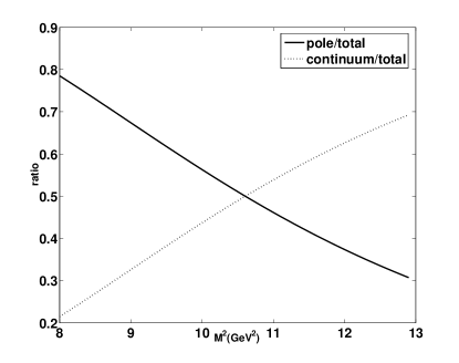
Figure 1: The solid line shows the relative pole contribution (the pole contribution divided by the total, pole plus continuum contribution) and the dashed line shows the relative continuum contribution for $Y_{b}(10890)$.

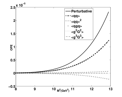
Figure 2: The OPE convergence is shown by comparing the perturbative, quark condensate, four-quark condensate, mixed condensate, two-gluon condensate, and three-gluon condensate contributions for $Y_{b}(10890)$.

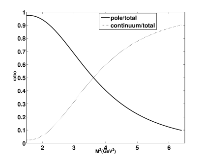
Figure 3: The solid line shows the relative pole contribution (the pole contribution divided by the total, pole plus continuum contribution) and the dashed line shows the relative continuum contribution for $Y(4360)$.

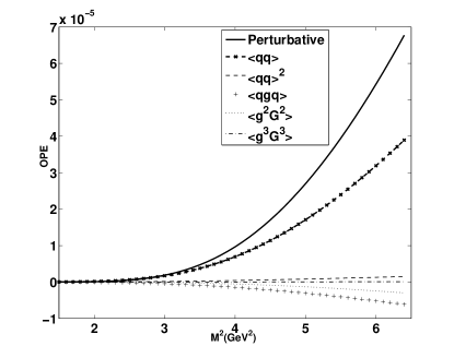
Figure 4: The OPE convergence is shown by comparing the perturbative, quark condensate, four-quark condensate, mixed condensate, two-gluon condensate, and three-gluon condensate contributions for $Y(4360)$.

Figure 5: The dependence on $M^{2}$ for the mass of $Y_{b}(10890)$ is shown.

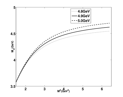
Figure 6: The dependence on $M^{2}$ for the mass of $Y(4360)$ is shown.

4 Summary

In the tentative P-wave $[bq][\bar{b}\bar{q}]$ configuration, the QCD sum rule method has been employed to compute the mass of $Y_{b}(10890)$, including the contributions of operators up to dimension six in the OPE. The numerical result $10.88\pm 0.13~{}\mbox{GeV}$ for $Y_{b}(10890)$ is well compatible with the experimental data, which favors the P-wave tetraquark configuration for $Y_{b}(10890)$. In the same picture, the mass of $Y(4360)$ has been calculated to be $4.32\pm 0.20~{}\mbox{GeV}$, and the result is in agreement with the experimental value, which supports its P-wave $[cq][\bar{c}\bar{q}]$ configuration. We expect the results could be helpful to understand the structures of these states. For further work, one needs to take into account other dynamical analysis to identify the structures of hadrons.

References

• [1] Belle Collaboration, K. F. Chen et al., Observation of anomalous $\Upsilon(1S)\pi^{+}\pi^{-}$ and $\Upsilon(2S)\pi^{+}\pi^{-}$ production near the $\Upsilon(5S)$ resonance, Phys. Rev. Lett. 100 (2008) 112001; Belle Collaboration, I. Adachi et al., Observation of an enhancement in $e^{+}e^{-}\rightarrow\Upsilon(1S)\pi^{+}\pi^{-}$, $Upsilon(2S)\pi^{+}\pi^{-}$, and $Upsilon(3S)\pi^{+}\pi^{-}$ production at Belle, hep-ex/0808.2445.
• [2] S. L. Olsen, Hadronic spectrum–multiquark states, Nucl. Phys. A 827 (2009) 53c; A. Zupanc, Hadron spectroscopy results from Belle, hep-ex/0910.3404.
• [3] W. S. Hou, Searching for the bottom counterparts of $X(3872)$ and $Y(4260)$ via $\pi^{+}\pi^{-}\Upsilon$, Phys. Rev. D 74 (2006) 017504; Y. A. Simonov, Di-Pion emission in heavy quarkonia decays, JETP Lett. 87 (2008) 121; C. Meng and K. T. Chao, Scalar resonance contributions to the dipion transition rates of $\Upsilon(4S,5S)$ in the rescattering model, Phys. Rev. D 77 (2008) 074003; C. Meng and K. T. Chao, Peak shifts due to $B^{*}-\bar{B}^{*}$ rescattering in $\Upsilon(5S)$ dipion transitions, Phys. Rev. D 78 (2008) 034022; M. Karliner and H. J. Lipkin, Possibility of exotic states in the Upsilon system, hep-ph/0802.0649.
• [4] A. Ali, C. Hambrock, and M. J. Aslam, A tetraquark interpretation of the Belle data on the anomalous $\Upsilon(1S)\pi^{+}\pi^{-}$ and $\Upsilon(2S)\pi^{+}\pi^{-}$ production near the $\Upsilon(5S)$ resonance, Phys. Rev. Lett. 104 (2010) 262001; A. Ali, C. Hambrock, I. Ahmed, and M. J. Aslam, A case for hidden $b\bar{b}$ tetraquarks based on $e^{+}e^{-}\rightarrow b\bar{b}$ cross section between $\sqrt{s}=10.54$ and $11.20~{}\mbox{GeV}$, Phys. Lett. B 684 (2010) 28.
• [5] BaBar Collaboration, B. Aubert et al., Measurement of the $e^{+}e^{-}\rightarrow b\bar{b}$ cross section between $\sqrt{s}=10.54$ and $11.20~{}\mbox{GeV}$, Phys. Rev. Lett. 102 (2009) 012001.
• [6] M. A. Shifman, A. I. Vainshtein, and V. I. Zakharov, QCD and resonance physics. Theoretical foundations, Nucl. Phys. B147 (1979) 385; QCD and resonance physics. Applications, B147 (1979) 448; V. A. Novikov, M. A. Shifman, A. I. Vainshtein, and V. I. Zakharov, Calculations in external fields in Quantum Chromodynamics. Technical review, Fortschr. Phys. 32 (1984) 585.
• [7] M. A. Shifman, Vacuum Structure and QCD Sum Rules, North-Holland, Amsterdam, (1992).
• [8] B. L. Ioffe, in “The spin structure of the nucleon”, edited by B. Frois, V. W. Hughes, N. de Groot, World Scientific, (1997), hep-ph/9511401.
• [9] S. Narison, QCD Spectral Sum Rules, World Scientific, Singapore, (1989).
• [10] P. Colangelo and A. Khodjamirian, in: M. Shifman (Ed.), At the Frontier of Particle Physics: Handbook of QCD, vol. 3, Boris Ioffe Festschrift, World Scientific, Sigapore, (2001), pp. 1495-1576, hep-ph/0010175; A. Khodjamirian, QCD sum rules - a working tool fro hadronic physics, (2002) hep-ph/0209166.
• [11] BaBar Collaboration, B. Aubert et al., Evidence of a broad structure at an invariant mass of $4:32~{}\mbox{GeV}$ in the reaction $e^{+}e^{-}\rightarrow\pi^{+}\pi^{-}\psi(2S)$ measured at BABAR, Phys. Rev. Lett. 98 (2007) 212001.
• [12] Belle Collaboration, X. L. Wang et al., Observation of two resonant structures in $e^{+}e^{-}\rightarrow\pi^{+}\pi^{-}\psi(2S)$ via initial-state radiation at Belle, Phys. Rev. Lett. 99 (2007) 142002.
• [13] Z. Q. Liu, X. S. Qin, and C. Z. Yuan, Combined fit to BABAR and Belle data on $e^{+}e^{-}\rightarrow\pi^{+}\pi^{-}\psi(2S)$, Phys. Rev. D 78 (2008) 014032.
• [14] X. Liu, X. Q. Zeng, and X. Q. Li, Possible molecule structure of the newly observed $Y(4260)$, Phys. Rev. D 72 (2005) 054023; Y. Cui, X. L. Chen, W. Z. Deng, and S. L. Zhu, The possible heavy tetraquarks $qQ\bar{q}\bar{Q}$, $qq\bar{Q}\bar{Q}$, and $qQ\bar{Q}\bar{Q}$, High Energy Phys. Nucl. Phys. 31 (2007) 7; S. L. Zhu, New Hadron States, Int. J. Mod. Phys. E 17 (2008) 283; S. L. Zhu, Spectroscopy of mesons with heavy quarks, Nucl. Phys. A 805 (2008) 221c.
• [15] C. Z. Yuan, P. Wang, and X. H. Mo, The $Y(4260)$ as an $\omega\chi_{c1}$ molecular state, Phys. Lett. B 634 (2006) 399; C. F. Qiao, One explanation for the exotic state $Y(4260)$, Phys. Lett. B 639(2006) 263; C. F. Qiao, A uniform description of the states recently observed at B-factories, J. Phys. G: Nucl. Part. Phys. 35 (2008) 075008; G. J. Ding, J. J. Zhu, and M. L. Yan, Canonical charmonium interpretation for $Y(4360)$ and $Y(4660)$, Phys. Rev. D 77(2008) 014033; Z. G. Wang, Mass spectrum of the scalar hidden charm and bottom tetraquark states, Phys. Rev. D 79 (2009) 094027.
• [16] K. K. Seth, Challenges in haron physics, hep-ex/0712.0340; D. Ebert, R. N. Faustov, and V. O. Galkin, Excited heavy tetraquarks with hidden charm, Eur. Phys. J. C 58 (2008) 399; J. Segovia, A. M. Yasser, D. R. Entem, and F. Fernández, $J^{PC}=1^{--}$ hidden charm resonances, Phys. Rev. D 78 (2008) 114033.
• [17] R. M. Albuquerque and M. Nielsen, QCD sum rules study of the $J^{PC}=1^{--}$ charmonium Y mesons, Nucl. Phys. A 815 (2009) 53.
• [18] M. Nielsen, F. S. Navarra, and S. H. Lee, New charmonium states in QCD sum rules: a concise review, hep-ph/0911.1958.
• [19] N. V. Drenska, R. Faccini, and A. D. Polosa, Higher tetraquark particles, Phys. Lett. B 669 (2008) 160.
• [20] H. Kim, S. H. Lee, and Y. Oh, Anticharmed pentaquark $\Theta_{c}(3099)$ from QCD sum rules, Phys. Lett. B 595 (2004) 293.
• [21] F. S. Navarra, M. Nielsen, and S. H. Lee, QCD sum rules study of $QQ\bar{u}\bar{d}$ mesons, Phys. Lett. B 649 (2007) 166.
• [22] L. J. Reinders, H. R. Rubinstein, and S. Yazaki, Hadron properties from QCD sum rules, Phys. Rep. 127 (1985) 1.
• [23] H. Y. Jin and J. G. Körner, Radiative corrections to the correlator of ($0^{++}$, $1^{-+}$) light hybrid currents, Phys. Rev. D 64 (2001) 074002; H. Y. Jin, J. G. Körner, and T. G. Steele, Improved determination of the mass of the $1^{+-}$ light hybrid meson from QCD sum rules, Phys. Rev. D 67 (2003) 014025.
• [24] Particle Data Group, C. Amsler et al., Review of particle physics, Phys. Lett. B 667 (2008) 1.